A Comparative Assessment of Machine-Learning Techniques for Land Use and Land Cover Classification of the Brazilian Tropical Savanna Using ALOS-2/PALSAR-2 Polarimetric Images


Abstract

1. Introduction
2. Materials and Methods
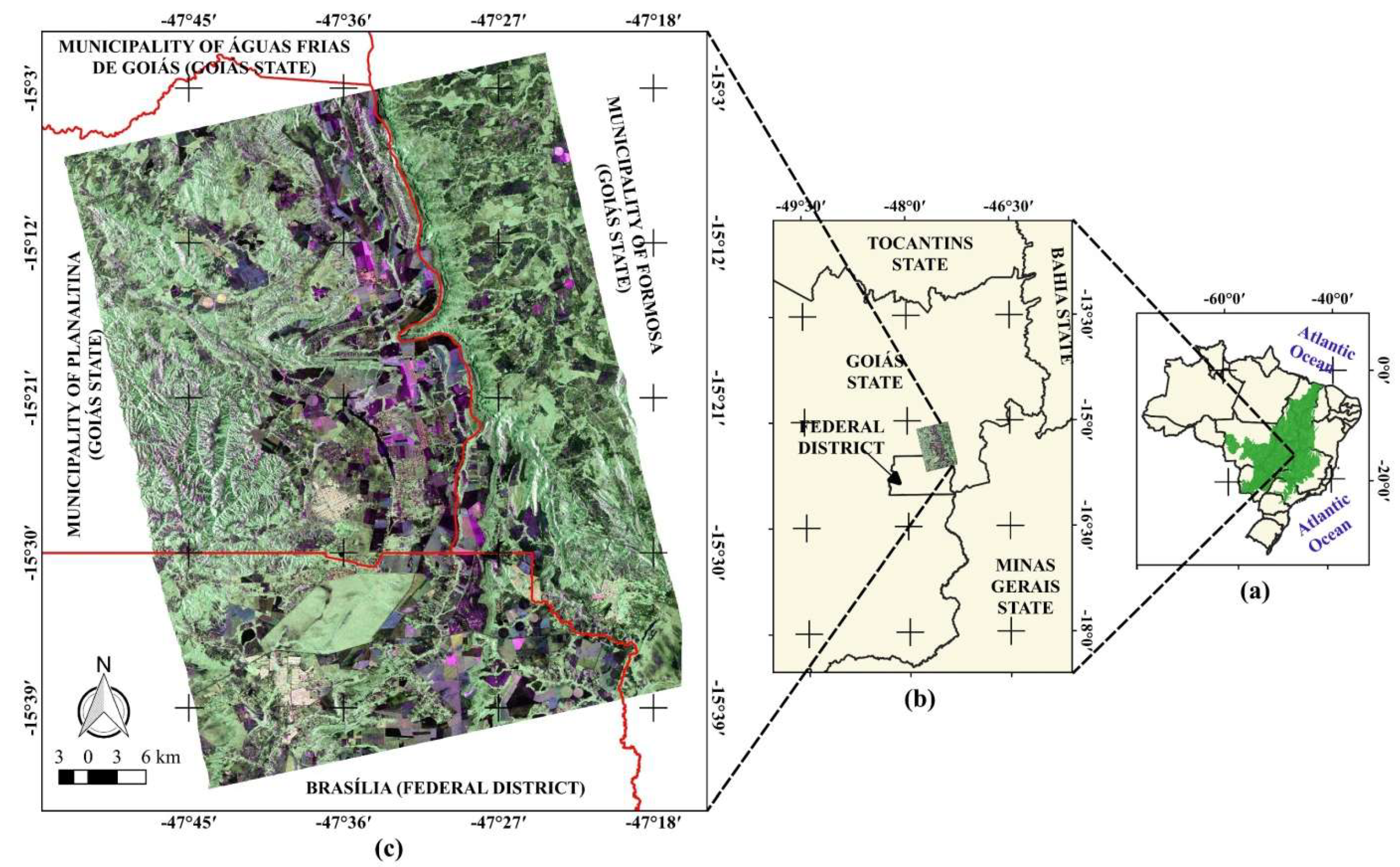
2.1. Study Area
2.2. Materials
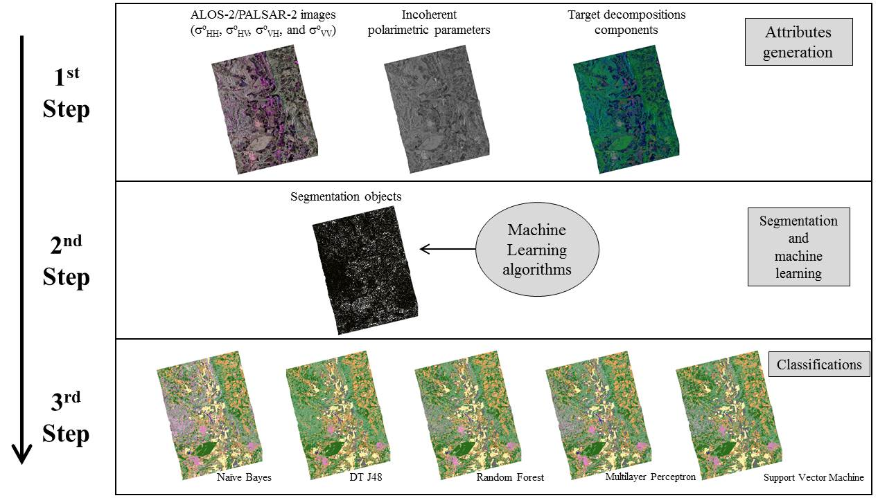
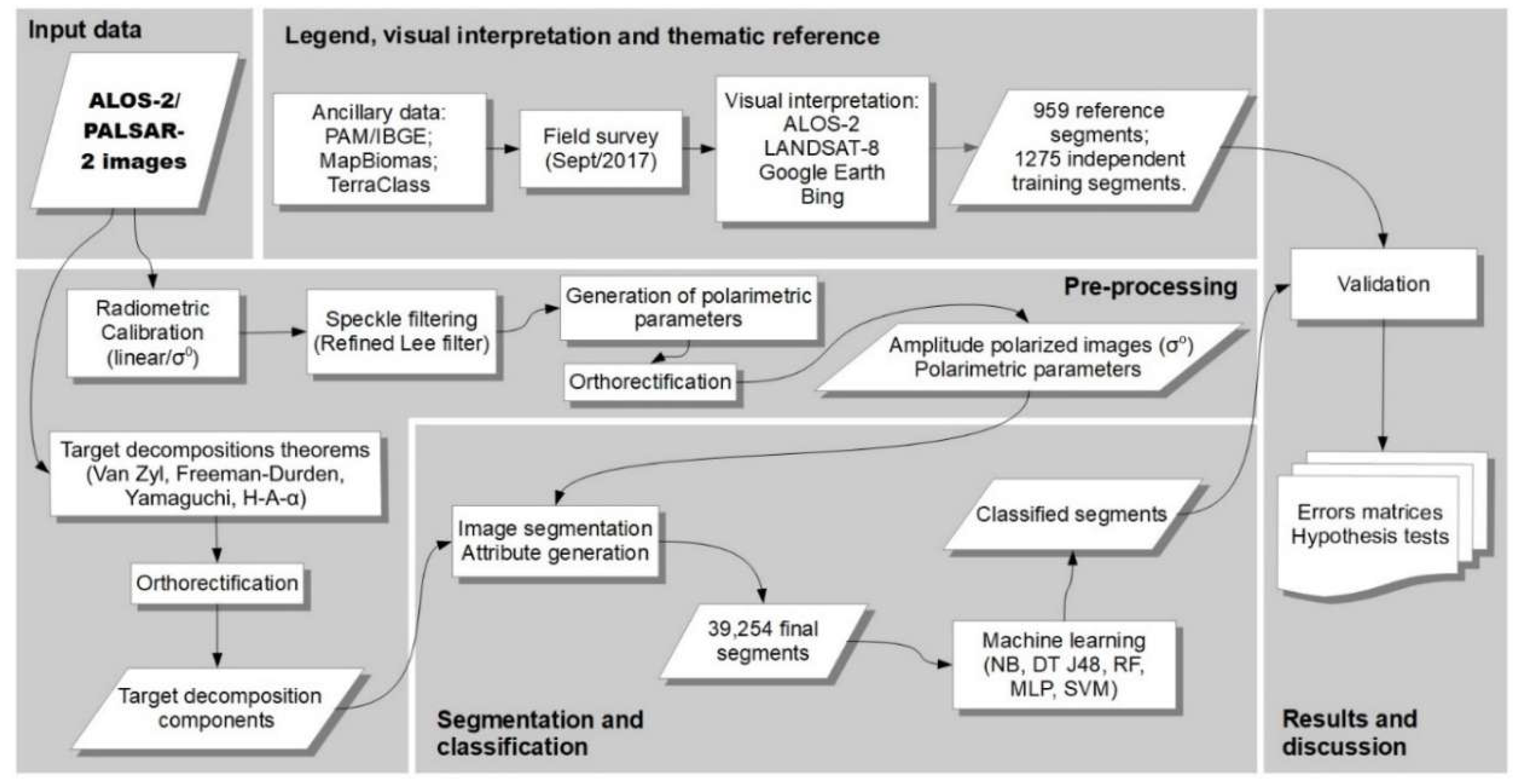
2.3. Approach
2.3.1. Preprocessing
2.3.2. Image Segmentation and Attribute Extraction
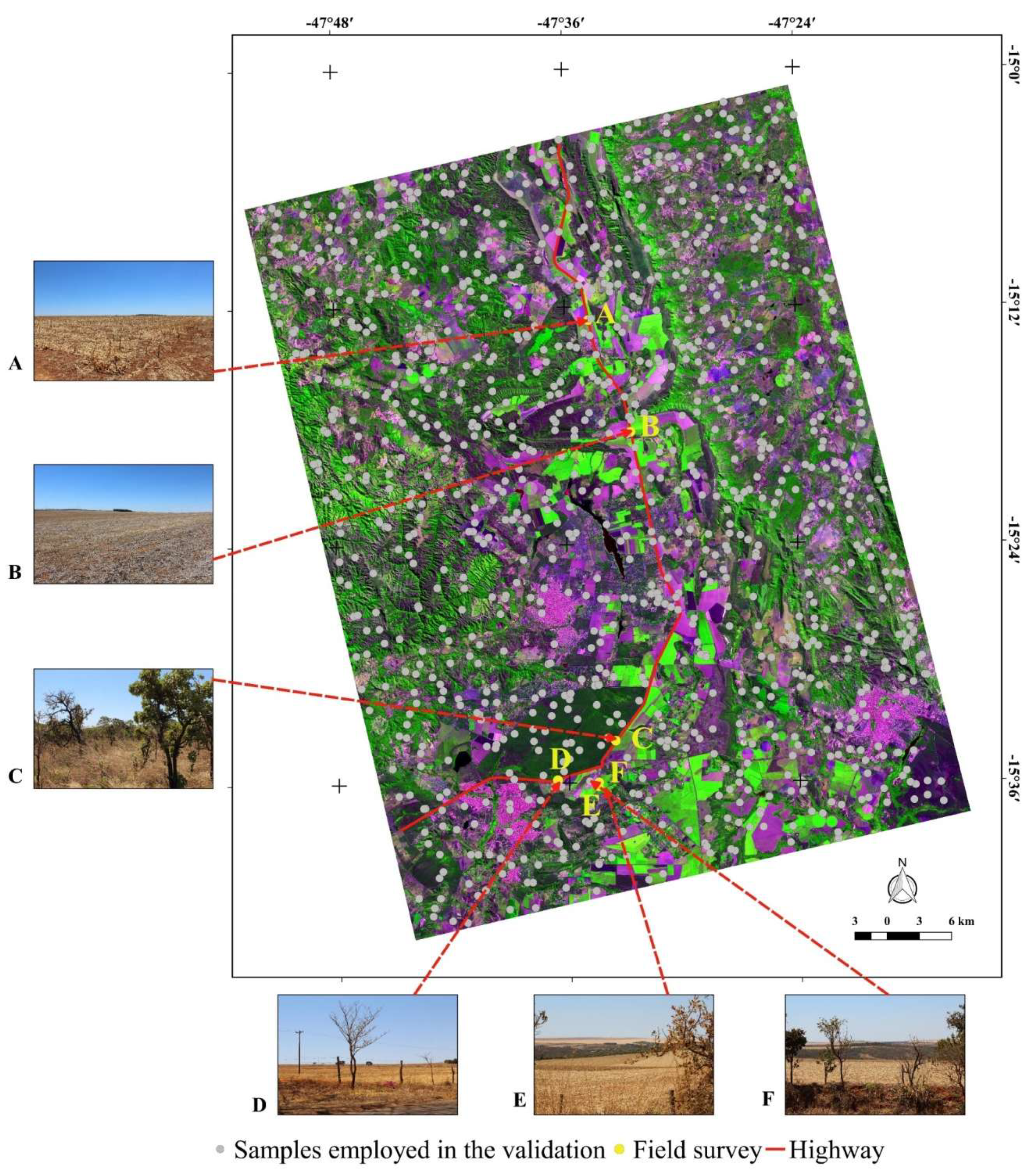
2.3.3. Classification and Validation
3. Results and Discussion
4. Conclusions
Author Contributions
Funding
Acknowledgments
Conflicts of Interest
References
- Gamba, P.; Aldrighi, M. SAR data classification of urban areas by means of segmentation techniques and ancillary optical data. IEEE J. Select. Top. Appl. Earth Obs. Remote Sens. 2012, 5, 1140–1148. [Google Scholar] [CrossRef]
- Qi, Z.; Yeh, A.G.O.; Li, X.; Lin, Z. A novel algorithm for land use and land cover classification using RADARSAT-2 polarimetric SAR data. Remote Sens. Environ. 2012, 118, 21–39. [Google Scholar] [CrossRef]
- Evans, T.L.; Costa, M. Landcover classification of the lower Nhecolândia subregion of the Brazilian Pantanal wetlands using ALOS/PALSAR, RADARSAT-2 and ENVISAT/ASAR imagery. Remote Sens. Environ. 2013, 128, 118–137. [Google Scholar] [CrossRef]
- Reynolds, J.; Wesson, K.; Desbiez, A.L.J.; Ochoa-Quintero, J.M.; Leimgruber, P. Using remote sensing and random forest to assess the conservation status of critical Cerrado habitats in Mato Grosso do Sul, Brazil. Land 2016, 5, 12. [Google Scholar] [CrossRef]
- Braun, A.; Hochschild, V. A SAR-based index for landscape changes in African savannas. Remote Sens. 2017, 9, 23. [Google Scholar] [CrossRef]
- Miles, L.; Kapos, V. Reducing greenhouse gas emissions from deforestation and forest degradation: Global land-use implications. Science 2008, 320, 1454–1455. [Google Scholar] [CrossRef] [PubMed]
- Haarpaintner, J.; Blanco, D.F.; Enssle, F.; Datta, P.; Mazinga, A.; Singa, C.; Mane, L. Tropical forest remote sensing services for the Democratic Republic of Congo inside the EU FP7 ‘Recover’ Project (Final Results 2000–2012). In Proceedings of the XXXVIth International Symposium on Remote Sensing of Environment, Berlin, Germany, 11–15 May 2015; pp. 397–402. [Google Scholar]
- Sano, E.E.; Rosa, R.; Brito, J.L.S.; Ferreira, L.G. Land cover mapping of the tropical savanna region in Brazil. Environ. Monit. Assess. 2010, 166, 113–124. [Google Scholar] [CrossRef] [PubMed]
- Scaramuzza, C.A.; Sano, E.E.; Adami, M.; Bolfe, E.L.; Coutinho, A.C.; Esquerdo, J.; Maurano, L.; Narvaes, I.D.S.; de Oliveira Filho, F.J.B.; Rosa, R.; et al. Land-use and land-cover mapping of the Brazilian Cerrado based mainly on Landsat-8 satellite images. Rev. Bras. Cart. 2017, 69, 1041–1051. [Google Scholar]
- Rahman, M.M.; Moran, M.S.; Thoma, D.P.; Bryant, R.; Collins, C.D.H.; Jackson, T.; Orr, B.J.; Tischler, M. Mapping surface roughness and soil moisture using multi-angle radar imagery without ancillary data. Remote Sens. Environ. 2008, 112, 391–402. [Google Scholar] [CrossRef]
- Duarte, R.M.; Wozniak, E.; Recondo, C.; Cabo, C.; Marquínez, J.; Fernández, S. Estimation of surface roughness and stone cover in burnt soils using SAR images. Catena 2008, 74, 264–272. [Google Scholar] [CrossRef]
- Tollerud, H.J.; Fantle, M.S. The temporal variability of centimeter-scale surface roughness in a playa dust source: Synthetic aperture radar investigation of playa surface dynamics. Remote Sens. Environ. 2014, 154, 285–297. [Google Scholar] [CrossRef]
- Bergen, K.M.; Goetz, S.J.; Dubayah, R.O.; Henebry, G.M.; Hunsaker, C.T.; Imhoff, M.L.; Nelson, R.F.; Parker, G.G.; Radeloff, V.C. Remote sensing of vegetation 3-D structure for biodiversity and habitat: Review and implications for lidar and radar spaceborne missions. J. Geophys. Res. 2009, 114, 1–13. [Google Scholar] [CrossRef]
- Jensen, J.R. Remote Sensing of the Environment. An Earth Resource Perspective, 2nd ed.; Prentice Hall: Upper Saddle River, NJ, USA, 2007. [Google Scholar]
- Myers, N.; Mittermeier, R.A.; Mittermeier, C.G.; Fonseca, G.A.B.; Kent, J. Biodiversity hotspots for conservation priorities. Nature 2000, 403, 853–858. [Google Scholar] [CrossRef] [PubMed]
- Strassburg, B.B.N.; Brooks, T.; Feltran-Barbiero, R.; Iribarrem, A.; Crouzeilles, R.; Loyola, R.; Latawiec, A.E.; Oliveira Filho, F.J.B.; Scaramuzza, C.A.M.; Scarano, F.R.; et al. Moment of truth for the Cerrado hotspot. Nat. Ecol. Evol. 2017, 1, 3. [Google Scholar] [CrossRef] [PubMed]
- Rada, N. Assessing Brazil’s Cerrado agricultural miracle. Food Policy 2013, 38, 146–155. [Google Scholar] [CrossRef]
- Sano, E.E.; Pinheiro, G.C.C.; Meneses, P.R. Assessing JERS-1 synthetic aperture radar data for vegetation mapping in the Brazilian savanna. J. Remote Sens. Soc. Jpn. 2001, 21, 158–167. [Google Scholar]
- Sano, E.E.; Ferreira, L.G.; Huete, A.R. Synthetic aperture radar (L-band) and optical vegetation indices for discriminating the Brazilian savanna physiognomies: A comparative analysis. Earth Interact. 2005, 9, 15. [Google Scholar] [CrossRef]
- Bitencourt, M.D.; Mesquita H.N., Jr.; Kuntschik, G.; Rocha, H.R.; Furley, P.A. Cerrado vegetation study using optical and radar remote sensing: Two Brazilian case studies. Can. J. Remote Sens. 2007, 33, 468–480. [Google Scholar] [CrossRef]
- Ningthoujam, R.K.; Balzter, H.; Tansey, K.; Feldpausch, T.R.; Mitchard, E.T.A.; Wani, A.A.; Joshi, P.K. Relationships of S-band radar backscatter and forest aboveground biomass in different forest types. Remote Sens. 2017, 9, 1116. [Google Scholar] [CrossRef]
- Bouvet, A.; Mermóz, S.; Le Toan, T.; Villard, L.; Mathieu, R.; Naidoo, L.; Asner, G.P. An above-ground biomass map of African savannahs and woodlands at 25m resolution derived from ALOS PALSAR. Remote Sens. Environ. 2018, 206, 156–173. [Google Scholar] [CrossRef]
- Odipo, V.O.; Nickless, A.; Berger, C.; Baade, J.; Urbazaev, M.; Walther, C.; Schmullius, C. Assessment of aboveground woody biomass dynamics using terrestrial laser scanner and L-band ALOS PALSAR data in South African savanna. Forests 2016, 7, 24. [Google Scholar] [CrossRef]
- Cassol, H.L.G.; Carreiras, J.M.B.; Moraes, E.C.; Aragão, L.E.O.C.; Silva, C.V.J.; Quegan, S.; Shimabukuro, Y.E. Retrieving secondary forest aboveground biomass from polarimetric ALOS-2 PALSAR-2 data in the Brazilian Amazon. Remote Sens. 2019, 11, 59. [Google Scholar] [CrossRef]
- Sano, E.E.; Santos, E.M.; Meneses, P.R. Análise de imagens do satélite ALOS PALSAR para o mapeamento de uso e cobertura da terra do Distrito Federal. Geociências 2009, 28, 441–451. [Google Scholar]
- Symeonakis, E.; Higginbottom, T.P.; Petroulaki, K.; Rabe, A. Optimisation of savannah land cover characterisation with optical and SAR data. Remote Sens. 2018, 10, 18. [Google Scholar] [CrossRef]
- Urbazaev, M.; Thiel, C.; Mathieu, R.; Naidoo, L.; Levick, S.R.; Smit, I.P.J.; Asner, G.P.; Schmullius, C. Assessment of the mapping of fractional woody cover in southern African savannas using multi-temporal and polarimetric ALOS PALSAR L-band images. Remote Sens. Environ. 2015, 166, 138–153. [Google Scholar] [CrossRef]
- Mendes, F.S.; Baron, D.; Gerold, G.; Liesenberg, V.; Erasmi, F. Optical and SAR remote sensing synergism for mapping vegetation types in the endangered Cerrado/Amazon ecotone of Nova Mutum—Mato Grosso. Remote Sens. 2019, 11, 1161. [Google Scholar] [CrossRef]
- INPE. Projeto TerraClass Cerrado. Mapeamento do uso e Cobertura Vegetal do Cerrado. 2017. Available online: http://www.dpi.inpe.br/tccerrado/download.php (accessed on 1 July 2017).
- MapBiomas. Mapeamento Anual da Cobertura e uso do Solo no Brasil. 2017. Available online: http://mapbiomas.org (accessed on 15 June 2017).
- IBGE. Produção Agrícola Municipal. 2017. Available online: https://ww2.ibge.gov.br/home/estatistica/economia/pam/2016/default.shtm (accessed on 10 August 2017).
- Ribeiro, J.F.; Walter, B.M.T. As principais fitofisionomias do Cerrado. In Cerrado: Ecologia e Flora; Sano, S.M., Almeida, S.P., Ribeiro, J.F., Eds.; Embrapa Cerrados: Planaltina, Brazil, 2008; pp. 151–199. [Google Scholar]
- Latrubese, E.M.; Carvalho, T.M. Geomorfologia do Estado de Goiás e Distrito Federal; Superintendência de Geologia e Mineração do Estado de Goiás: Goiânia, Brazil, 2006; 128p. [Google Scholar]
- USGS. Global Visualization (GloVis) Viewer. 2017. Available online: https://glovis.usgs.gov/ (accessed on 5 February 2017).
- INMET. Estações Automáticas. DF—Águas Emendadas. 2018. Available online: http://www.inmet.gov.br/portal/index.php?r=estacoes/estacoesAutomaticas (accessed on 15 July 2018).
- JAXA. Calibration Results of Alos-2/Palsar-2 Jaxa Standard Products. 2018. Available online: https://www.eorc.jaxa.jp/ALOS-2/en/calval/calval_index.htm (accessed on 15 January 2018).
- Lee, J.; Pottier, E. Polarimetric Radar Imaging. In From Basics to Applications; CRC Press: Boca Raton, FL, USA, 2009. [Google Scholar]
- Boerner, W.; Mott, H.; Lünenberg, E.; Livingstone, C.; Brisco, B.; Brown, R.J.; Paterson, J.S. Polarimetry in radar remote sensing: Basic and applied concepts. In Manual of Remote Sensing: Principles and Applications of Imaging Radars, 3rd ed.; Henderson, F.M., Lewis, A.J., Eds.; John Wiley & Sons: New York, NY, USA, 1998; pp. 271–356. [Google Scholar]
- Kim, Y.; van Zyl, J.J. A time-series approach to estimate soil moisture using polarimetric radar data. IEEE Trans. Geosci. Remote Sens. 2009, 47, 2519–2527. [Google Scholar] [CrossRef]
- Mitchard, E.T.A.; Saatchi, S.S.; White, L.J.T.; Abernethy, K.A.; Jeffery, K.J.; Lewis, S.L.; Collins, M.; Lefsky, M.A.; Leal, M.E.; Woodhouse, I.H.; et al. Mapping tropical forest biomass with radar and spaceborne LIDAR in Lopé National Park, Gabon: Overcoming problems of high biomass and persistent cloud. Biogeosciences 2012, 9, 179–191. [Google Scholar] [CrossRef]
- Pope, K.O.; Rey-Benayas, J.M.; Paris, J.F. Radar remote sensing of forest and wetland ecosystems in the central American tropics. Remote Sens. Environ. 1994, 48, 205–219. [Google Scholar] [CrossRef]
- Cloude, S.R.; Pottier, E. A review of target decomposition theorems in radar polarimetry. IEEE Trans. Geosci. Remote Sens. 1996, 34, 498–518. [Google Scholar] [CrossRef]
- Hellmann, M.P. SAR Polarimetry Tutorial. 2001. Available online: http://epsilon.nought.de/ (accessed on 1 February 2017).
- Richards, J.A. Remote Sensing with Imaging Radar; Springer: Berlin, Germany, 2009. [Google Scholar]
- van Zyl, J.J. Unsupervised classification of scattering behavior using radar polarimetry data. IEEE Trans. Geosci. Remote Sens. 1989, 27, 36–45. [Google Scholar] [CrossRef]
- Freeman, A.; Durden, S.L. A three-component scattering model for polarimetric SAR Data. IEEE Trans. Geosci. Remote Sens. 1998, 36, 963–973. [Google Scholar] [CrossRef]
- Yamaguchi, Y.; Moriyama, T.; Ishido, M.; Yamada, H. Four-component scattering model for polarimetric SAR image decomposition. IEEE Trans. Geosci. Remote Sens. 2005, 43, 1699–1706. [Google Scholar] [CrossRef]
- Trimble. eCognition Developer 8.7. Reference Book; Trimble: Munich, Germany, 2011. [Google Scholar]
- Benz, U.C.; Hofmann, P.; Willhauck, G.; Lingenfelder, I.; Heynen, M. Multi-resolution, object-oriented fuzzy analysis of remote sensing data for GIS ready information. ISPRS J. Photogramm. Remote Sens. 2004, 58, 239–258. [Google Scholar] [CrossRef]
- Zhang, H. The Optimality of Naive Bayes. Available online: http://www.cs.unb.ca/~hzhang/publications/ FLAIRS04ZhangH.pdf (accessed on 13 June 2019).
- Caruana, R.; Niculescu-Mizil, A. An Empirical Comparison of Supervised Learning Algorithms. Available online: http://www.cs.cornell.edu/~caruana/ctp/ct.papers/caruana.icml06.pdf (accessed on 13 June 2019).
- John, G.H.; Langley, P. Estimating Continuous Distributions in Bayesian Classifiers. In Proceedings of the Eleventh Conference on Uncertainty in Artificial Intelligence, Montreal, QC, Canada, 18–20 August 1995; Morgan Kaufmann: San Mateo, CA, USA; pp. 338–345. Available online: http://web.cs.iastate.edu/~honavar/bayes-continuous.pdf (accessed on 13 June 2019).
- Quinlan, J.R. Combining instance-based and model-based learning. In Proceedings of the Tenth International Conference on Machine Learning, Amherst, MA, USA, 27–29 June 1993; pp. 236–243. [Google Scholar]
- Hastie, T.J.; Tibshirani, R.J.; Friedman, J.H. The Elements of Statistical Learning: Data Mining, Inference, and Prediction; Springer: New York, NY, USA, 2009. [Google Scholar]
- Belgiu, M.; Dragut, L. Random forest in remote sensing: A review of applications and future directions. ISPRS J. Photogramm. 2016, 114, 24–31. [Google Scholar] [CrossRef]
- Rodriguez-Galiano, V.F.; Chica-Rivas, M. Evaluation of different machine learning methods for land cover mapping of a Mediterranean area using multi-seasonal Landsat images and Digital Terrain Models. Int. J. Digit. Earth. 2014, 7, 492–509. [Google Scholar] [CrossRef]
- Breiman, L. Random Forests. Mach. Learn. 2001, 45, 5–32. [Google Scholar] [CrossRef]
- Win, T.S.; Malik, A.A.; Prachayasittikul, V.; Wikberg, J.E.S.; Nantasenamat, C.; Shoombuatong, W. HemoPred: A web server for predicting the hemolytic activity of peptides. Future Med. Chem. 2017, 9, 275–291. [Google Scholar] [CrossRef] [PubMed]
- Win, T.S.; Schaduangrat, N.; Prachayasittikul, V.; Nantasenamat, C.; Shoombuatong, W. PAAP: A web server for predicting antihypertensive activity of peptides. Future Med. Chem. 2018, 10, 1749–1767. [Google Scholar] [CrossRef] [PubMed]
- Zhang, Q.; Gao, W.; Su, S.; Weng, M.; Cai, Z. Biophysical and socioeconomic determinants of tea expansion: Apportioning their relative importance for sustainable land use policy. Land Use Policy 2017, 68, 438–447. [Google Scholar] [CrossRef]
- Hu, L.; He, S.; Han, Z.; Xiao, H.; Su, S.; Weng, M.; Cai, Z. Monitoring housing rental prices based on social media: An integrated approach of machine-learning algorithms and hedonic modeling to inform equitable housing policies. Land Use Policy 2019, 82, 657–673. [Google Scholar] [CrossRef]
- Haykin, S.S. Neural Networks: A Comprehensive Foundation; Prentice-Hall: Upper Saddle River, NJ, USA, 1999. [Google Scholar]
- Lian, C.; Zeng, Z.; Yao, W.; Tang, H. Multiple neural networks switched prediction for landslide displacement. Eng. Geol. 2015, 186, 91–99. [Google Scholar] [CrossRef]
- Bishop, C.M. Neural Networks for Pattern Recognition; Oxford University Press: Oxford, UK, 1995. [Google Scholar]
- Fischer, M.M.; Abrahart, R.J. Neurocomputing—Tools for Geographers. In GeoComputation; Openshaw, S., Abrahart, R.J., Eds.; Taylor & Francis: New York, NY, USA, 2000; pp. 187–217. [Google Scholar]
- Li, G.; Cai, Z.; Liu, X.; Liu, J.; Su, S. A comparison of machine learning approaches for identifying high-poverty counties: Robust features of DMSP/OLS night-time light imagery. Int. J. Remote Sens. 2019, 40, 5716–5736. [Google Scholar] [CrossRef]
- Witten, I.H.; Frank, E. Data Mining: Practical Machine Learning. Tools and Techniques, 2nd ed.; Morgan Kaufmann: San Francisco, CA, USA, 2005. [Google Scholar]
- Han, J.; Kamber, M.; Pei, J. Data Mining: Concepts and Techniques, 3rd ed.; Elsevier: Whaltan, MA, USA, 2012. [Google Scholar]
- Congalton, R.G.; Green, K. Assessing the Accuracy of Remotely Sensed Data: Principles and Practices; CRC Press: Boca Raton, FL, USA, 2009. [Google Scholar]
- Shiraishi, T.; Motohka, T.; Thapa, R.B.; Watanabe, M.; Shimada, M. Comparative assessment of supervised classifiers for land use-land cover classification in a tropical region using time-series PALSAR mosaic data. IEEE J. Select. Top. Appl. Earth Obs. Remote Sens. 2014, 7, 1186–1199. [Google Scholar] [CrossRef]
- Landis, J.R.; Koch, G.G. The measurement of observer agreement for categorical data. Biometrics 1977, 33, 159–174. [Google Scholar] [CrossRef]


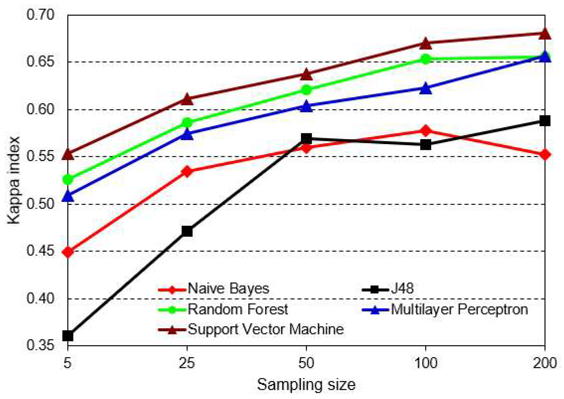
| Statistics | Mean of Kappa Indices | Standard Deviation of Kappa Indices | |
|---|---|---|---|
| ML Classifiers | Naive Bayes | 0.53454 | 0.050026823 |
| J48 | 0.51036 | 0.095230893 | |
| Random Forest | 0.6084 | 0.054270802 | |
| Multilayer Perceptron | 0.59344 | 0.055937715 | |
| Support Vector Machine | 0.63064 | 0.051343188 | |
| Classifier | NB | DT J48 | RF | MLP | SVM |
|---|---|---|---|---|---|
| NB | - | 0.0838 | 0.0000 | 0.0000 | 0.0000 |
| DT J48 | 0.0838 | - | 0.0046 | 0.0038 | 0.0001 |
| RF | 0.0000 | 0.0046 | - | 0.4790 | 0.1565 |
| MLP | 0.0000 | 0.0038 | 0.4790 | - | 0.1673 |
| SVM | 0.0000 | 0.0001 | 0.1565 | 0.1673 | - |
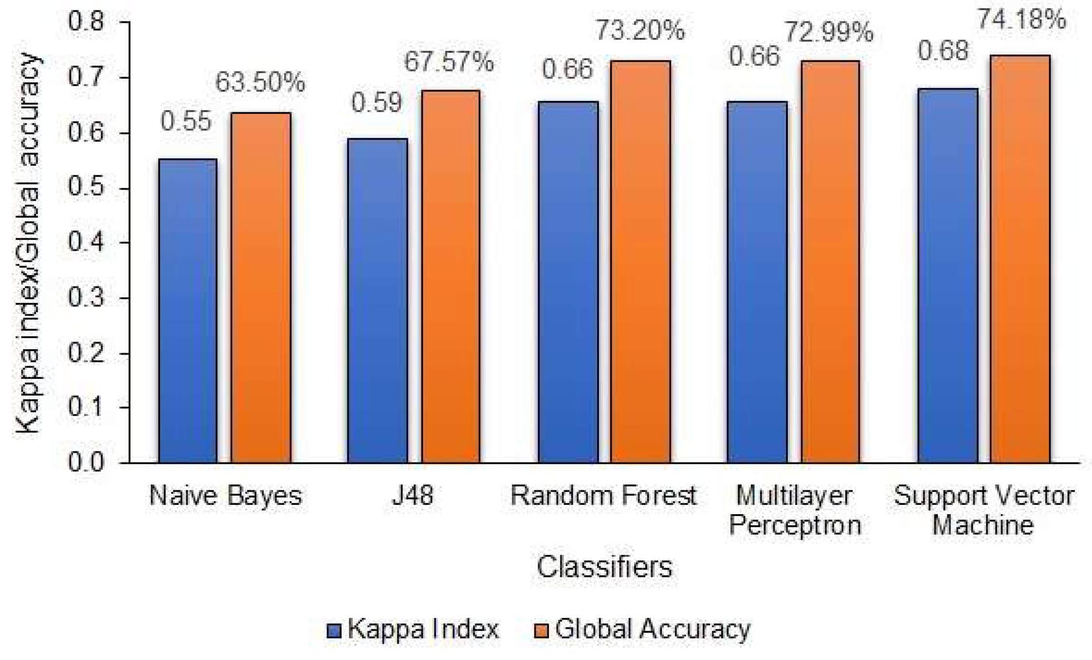
| Rank | Classifier | Kappa Index | Global Accuracy (%) |
|---|---|---|---|
| 1st | SVM | 0.68 | 74.18 |
| RF | 0.66 | 73.20 | |
| MLP | 0.66 | 72.99 | |
| 2nd | DT J48 | 0.59 | 65.57 |
| NB | 0.55 | 63.50 |
© 2019 by the authors. Licensee MDPI, Basel, Switzerland. This article is an open access article distributed under the terms and conditions of the Creative Commons Attribution (CC BY) license (http://creativecommons.org/licenses/by/4.0/).
Share and Cite
Camargo, F.F.; Sano, E.E.; Almeida, C.M.; Mura, J.C.; Almeida, T. A Comparative Assessment of Machine-Learning Techniques for Land Use and Land Cover Classification of the Brazilian Tropical Savanna Using ALOS-2/PALSAR-2 Polarimetric Images. Remote Sens. 2019, 11, 1600. https://doi.org/10.3390/rs11131600
Camargo FF, Sano EE, Almeida CM, Mura JC, Almeida T. A Comparative Assessment of Machine-Learning Techniques for Land Use and Land Cover Classification of the Brazilian Tropical Savanna Using ALOS-2/PALSAR-2 Polarimetric Images. Remote Sensing. 2019; 11(13):1600. https://doi.org/10.3390/rs11131600
Chicago/Turabian StyleCamargo, Flávio F., Edson E. Sano, Cláudia M. Almeida, José C. Mura, and Tati Almeida. 2019. "A Comparative Assessment of Machine-Learning Techniques for Land Use and Land Cover Classification of the Brazilian Tropical Savanna Using ALOS-2/PALSAR-2 Polarimetric Images" Remote Sensing 11, no. 13: 1600. https://doi.org/10.3390/rs11131600
APA StyleCamargo, F. F., Sano, E. E., Almeida, C. M., Mura, J. C., & Almeida, T. (2019). A Comparative Assessment of Machine-Learning Techniques for Land Use and Land Cover Classification of the Brazilian Tropical Savanna Using ALOS-2/PALSAR-2 Polarimetric Images. Remote Sensing, 11(13), 1600. https://doi.org/10.3390/rs11131600