Article

Sinkhole Detection and Characterization Using LiDAR-Derived DEM with Logistic Regression

1
Department of Civil, Environmental, and Construction Engineering, University of Central Florida, Orlando, FL 32816, USA
2
Department of Civil Engineering, Hongik University, Seoul 04066, Korea
*
Author to whom correspondence should be addressed.
Remote Sens. 2019, 11(13), 1592; https://doi.org/10.3390/rs11131592
Submission received: 2 May 2019 / Revised: 25 June 2019 / Accepted: 29 June 2019 / Published: 4 July 2019
(This article belongs to the Section Remote Sensing in Geology, Geomorphology and Hydrology)

Abstract

:
Depressions due to sinkhole formation cause significant structural damages to buildings and civil infrastructure. Traditionally, visual inspection has been used to detect sinkholes, which is a subjective way and time- and labor-consuming. Remote sensing techniques have been introduced for morphometric studies of karst landscapes. This study presents a methodology for the probabilistic detection of sinkholes using LiDAR-derived digital elevation model (DEM) data. The proposed study provides benefits associated with: (1) Detection of unreported sinkholes in rural and/or inaccessible areas, (2) automatic delineation of sinkhole boundaries, and (3) quantification of the geometric characteristics of those identified sinkholes. Among sixteen morphometric parameters, nine parameters were chosen for logistic regression, which was then employed to compute the probability of sinkhole detection; a cutoff value was back-calculated such that the sinkhole susceptibility map well predicted the reported sinkhole boundaries. According to the results of the LR model, the optimal cutoff value was calculated to be 0.13, and the area under the curve (AUC) of the receiver operating characteristic curve (ROC) was 0.90, indicating the model is reliable for the study area. For those identified sinkholes, the geometric characteristics (e.g., depth, length, area, and volume) were computed.

1. Introduction

Sinkholes can cause serious damage to properties and infrastructure, and sometimes human casualties occur in severe cases. In the United States, economic damage due to sinkholes has been estimated to be over $300 million per year and the actual damage is likely to be much greater than this estimate [1]. Considerable damage from natural sinkholes is particularly common in Florida, Texas, Alabama, Missouri, Kentucky, Tennessee, and Pennsylvania [2]. Insurers in Florida, the most vulnerable state to sinkhole damage, received a total of 24,671 claims for sinkhole damage between 2006 and 2010, totaling $1.4 billion [3]. According to the Florida Office of Insurance Regulation (FLOIR) report, the insurers’ expense has been gradually growing with increases in both frequency and severity of sinkholes.
Sinkholes have been classified into two main groups [4,5]. The first group, known as solution sinkholes, involves centripetal flow to areas having the highest permeability and consequent dissolution [6,7,8]. The second group is known as subsidence sinkholes and involves downward movement of overlying soils into cavities within bedrock. Subsidence sinkholes are further classified using two descriptors: The material affected by internal erosion or deformation (cover, bedrock, and caprock) and the main subsidence mechanism (collapse, suffosion, or sagging). Details of sinkhole classification can be found in previous research by Gutiérrez et al. [5].
Some researchers reported that morphometric parameters of sinkholes vary significantly and they depend on the different types and formation processes of sinkholes [9,10]. Traditionally, topographic maps and aerial photographs were used to investigate karst landscapes and digital elevation models (DEMs) were used in morphometric studies [11]. However, DEMs have relatively low levels of resolution and accuracy, which is made worse in forested areas [12].
Airborne light detection and ranging (LiDAR) (or airborne laser scanning) can penetrate forest and construct the topography of the underlying terrain [13,14]. In addition, high-resolution LiDAR data enables more accurate and delineation analyses of ground features and geomorphology of landscapes [15,16].
Recently, LiDAR data have been used to detect and characterize sinkholes. Filin et al. [17] applied LiDAR for 3D characterization of sinkholes in the Dead Sea area and delineated sinkholes. Kobal et al. [18] presented a case study to map and explore the geomorphometric characteristics of sinkholes under forest cover by utilizing a digital elevation model derived from airborne laser scanning data. Mukherjee and Zachos [19] used a sink-filling method to delineate depression boundaries. In their study, sinkholes were extracted by applying different thresholds to the results. Zhu et al. [20] employed a similar sink-filling method to process LiDAR data and found that four times more potential sinkholes would be identified than the existing sinkhole data for the same area. Several researchers have proposed image processing techniques to detect and delineate sinkhole boundaries. Obu and Podobnikar [21] introduced kernel windows using focal functions to automate sinkhole recognition. Rahimi and Alexander Jr [22] implemented the active contour method to delineate karst sinkhole boundaries based on seed points.
This study presents a probabilistic LiDAR-based assessment for sinkhole identification and assessment of sinkhole characteristics. Logistic regression was employed to the LiDAR data to compute the probability of sinkhole detection. Logistic regression is a widely adopted method for the assessment of various geohazards, including landslides, floods, volcano eruptions, and soil erosion [23,24,25,26], and for the development of sinkhole susceptibility maps [27,28,29]. In this study, all related morphometric indices were statistically checked and the critical contributing variables were selected for the logistic regression model. The identified sinkholes were validated using a sinkhole database; once sinkholes were identified, the geometric characteristics of those identified sinkholes were computed.

2. Study Area

The study area is located in the Springfield Plateau region, the southwestern part of the state of Missouri, and more specifically in Greene County (Figure 1). It is located between latitudes 37°18′00″ N and 37°19′40″ N and longitudes 93°20′30″ W and 93°22′30″ W, with an area of 9 km2. The estimated terrain elevation above sea level ranges between 327 and 381 m. The region is underlain by thick and well karstified carbonate rocks that develop a variety of karst features, including sinkholes, caves, and springs. The process of sinkhole formation and collapse in this region is due to dissolution and cavity growth in the underlying bedrock as groundwater percolates through voids and cracks in the rock. According to the Geological Survey Program of the Missouri Department of Natural Resources’ Missouri Geological Survey, 15,763 sinkholes have been reported in the state until December 2018 and numerous non-reported sinkholes also exist in the region [30]. In the study area, a total of 199 sinkholes of varying sizes have been identified.

3. Methodology

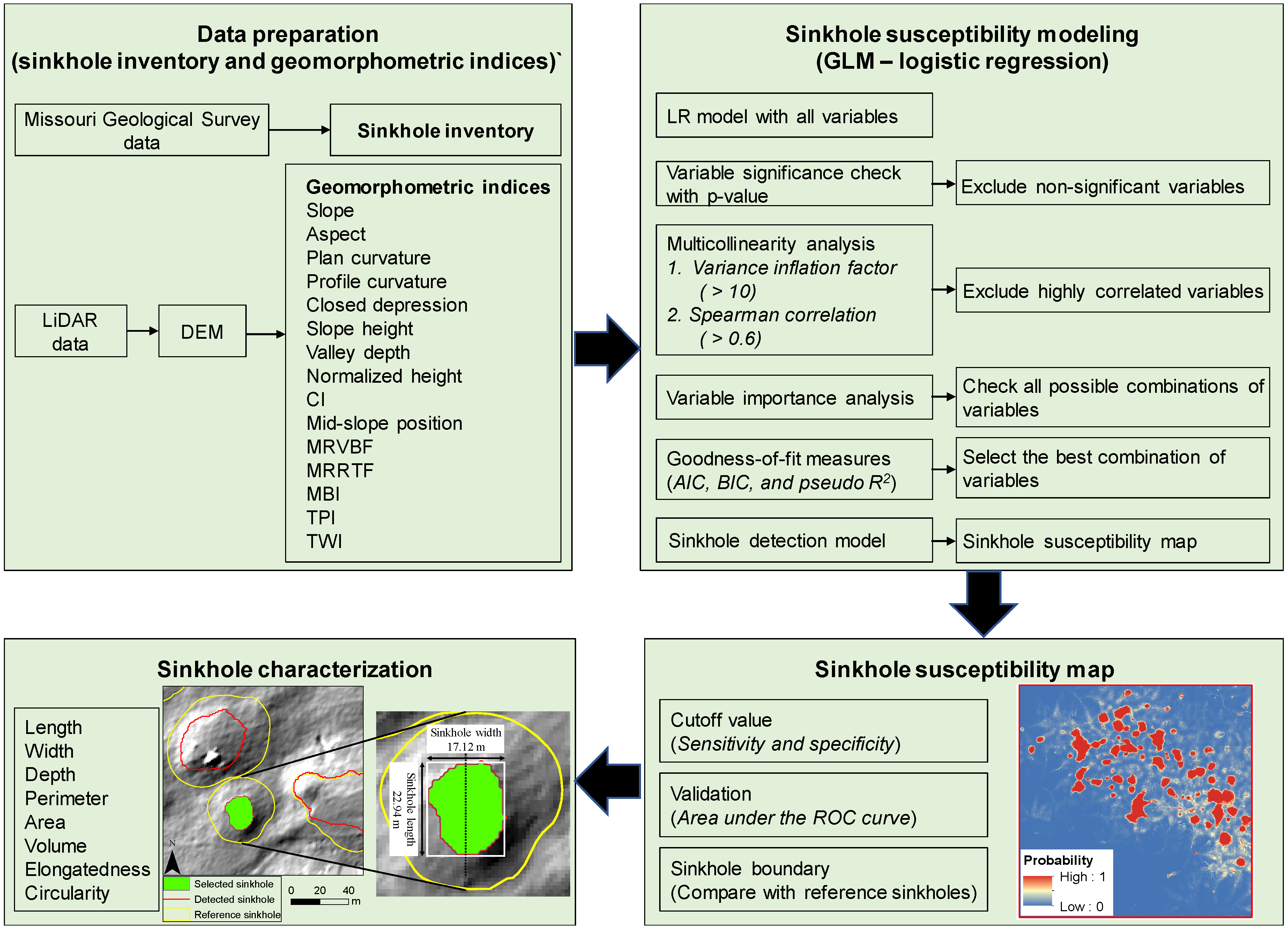
The flow chart showing the research methodology is presented in Figure 2. This study mainly consists of the following four steps: (1) Data preparation; (2) sinkhole susceptibility modeling using the generalized linear model (GLM) for logistic regression (LR); (3) sinkhole susceptibility mapping to detect sinkhole boundaries; and (4) sinkhole geometric characterization. In the data preparation step, a digital elevation model (DEM) and geomorphometric indices were created. Logistic regression was then selected for the sinkhole susceptibility model. A sinkhole susceptibility map was created through the cutoff value identified. Once the boundaries of sinkholes were identified, geometric characteristics such as length, area, volume, and circularity were determined. Details of each step are presented below.

3.1. Data Preparation

A DEM is a regularly spaced grid of terrain elevation and is created from LiDAR datasets using GIS software. This high-resolution DEM is a fundamental element of sinkhole inventories, and the Missouri Department of Natural Resources (MDNR) actively uses a LiDAR-derived DEM to identify sinkhole boundaries. For this study, a DEM at a resolution of 1 m was acquired from the Missouri LiDAR DEM Download Tool of the Missouri Spatial Data Information Service [31]. The airborne LiDAR dataset for the study area was collected in 2007 using the Leica ALS-60 LiDAR system. The estimate of accuracy of LiDAR data is documented as 15 cm for vertical and 50 cm for horizontal accuracy [32]. While the resolution of the constructed DEM is different from the LiDAR point cloud data (which is stored in an LAS file format), it is the best available resolution and high enough to detect and map sinkholes.
Commonly used geomorphometric indices (or parameters) were derived using SAGA GIS software (http://saga-gis.org) and then included as independent variables in the GLM model building process [33]. The LiDAR-based DEM was used to extract the remaining indices. The following 16 indices were derived from the DEM: Slope, aspect, plan curvature, profile curvature, closed depression, slope height, valley depth, normalized height, convergence index (search radius of 50 m), convergence index (search radius of 100 m), mid-slope position, multiresolution index of valley bottom flatness (MRVBF), multiresolution ridge top flatness index (MRRTF), mass balance index (MBI), topographic position index (TPI), and topographic wetness index (TWI). These indices are defined as:
  • Slope: Slope is one of the most important factors in hydrology because it is related to surface and subsurface flow velocity and runoff rate over the area of interest [34,35]. As slope increases, time for surface infiltration decreases, resulting in an increase in soil erosion. In this study area, the slope ranges from 0 to 81.6° (0 to 680% in percent rise). Steep slopes are located within the southwest area along the Little Sac River.
  • Aspect: Aspect (or slope aspect) refers to the primary direction of change of a DEM and is expressed in degrees in a clockwise direction from north (ArcGIS 2010). The slope aspect affects exposure to rainfall, wind, and vegetation cover of the area [34,35].
  • Plan curvature (PLC): PLC is the rate of change in aspect. A positive curvature indicates an upwardly convex surface of that cell, while a negative curvature indicates an upwardly concave surface of that cell. A value of 0 refers to flat surface [34,36,37].
  • Profile curvature (PRC): PRC is the rate of change in gradient [34,36,37].
  • Closed depression (CD): The boundary of a depression is defined as the spatial extent of maximum water surface level when the depression is filled with flood water and then starts spilling out. Therefore, a closed depression can be a significant indicator of a sinkhole boundary in karst landscapes.
  • Slope height (SH): SH is defined as the relative height above the closest modeled drainage accumulation [38,39]. It ranged from 0 to 29 m for the study area.
  • Valley depth (VD): VD is the vertical height below summit accumulation [38]. It ranged from 0 to 27 m for the study area.
  • Normalized height (NH): NH is the normalized difference between SH and the VD and is unitless [38,39].
  • Convergence index (CI50, 50-m search radius): CI50 is used to determine whether water flow from neighboring cells diverges or converges. Convergence is calculated using flow direction between adjacent cells based on the aspects of neighboring cells [40].
  • Convergence index (CI100, 100-m search radius): The same CI but the search radius of 100 m was used.
  • Mid-slope position (MSP): MSP has values ranging from 0 (minimum slope) to 1 (maximum vertical distance from valley bottom or ridge top, i.e., valleys and crests) [41].
  • Multiresolution index of valley bottom flatness (MRVBF): MRVBF is a measure of flatness and lowness depicting depositional areas [42]. Higher values correspond to larger valleys. It ranged from 0 to 4.99 for the study area.
  • Multiresolution ridge top flatness index (MRRTF): MRRTF is a measure of flatness and elevation, depicting stable upland areas [42]. Higher values correspond to ridges. It ranged from 0 to 5.67 for the study area.
  • Mass balance index (MBI): MBI is derived from transformed elevation, slope, and mean curvature. Positive values indicate convex forms (upper slopes, crests) whereas negative values indicate concave forms (valleys and lower slopes) [43].
  • Topographic position index (TPI): TPI is the difference between a raster cell elevation and the average elevation of neighboring cells. TPI is calculated as:
    T P I = Z o Z ¯
    Z ¯ = 1 n R Z o ( i R )
    where Z o is the elevation at a central point and Z ¯ is the mean surrounding elevation. Positive TPI values denote that the cell is located higher than its average neighborhood, whereas negative values denote that the cell is in lower position [35,44].
  • Topographic wetness index (TWI): TWI combines the local upslope contributing area and slope. TWI is calculated as:
    T W I = l n ( α t a n β )
    where α is the upslope catchment area per unit contour length and β is the local slope gradient in percentage. High values indicate drainage depressions whereas low values indicate crest and ridges [45]. For more detailed information, you can find them at Supplementary Materials.
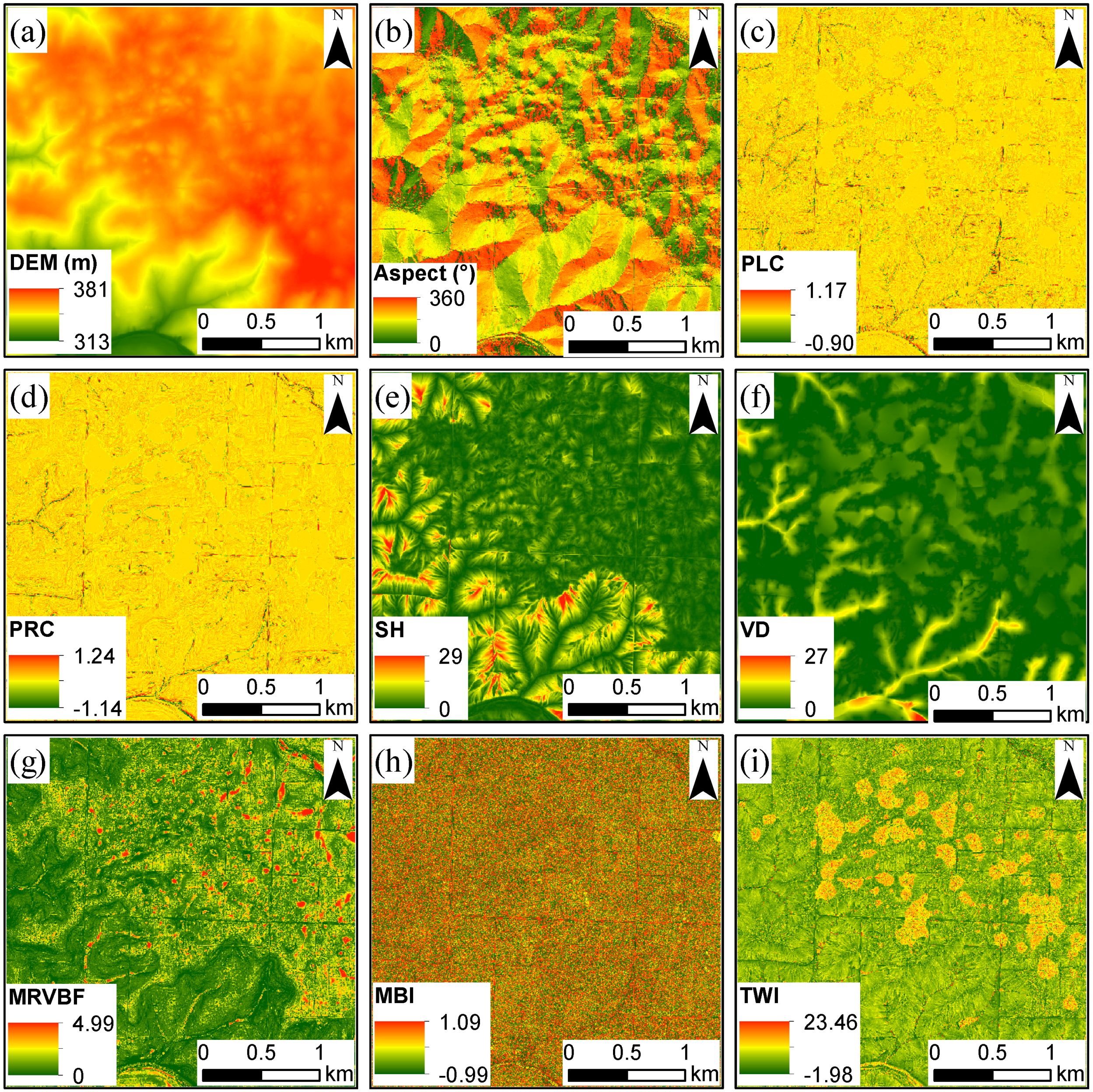
Figure 3 shows the map of 9 geomorphometric indices used for the final model development. While 16 indices were considered as significant contributing indices to the sinkhole susceptibility map, 7 indices were excluded by eliminating insignificant variables and/or highly correlated variables. Details of such a process will be discussed in Section 4.1. All maps were produced with a spatial resolution of 1 m.

3.2. GLM Model Selection—Logistic Regression

Generalized linear modeling (GLM) was employed to determine the existence of sinkholes, which was necessary for generating the probabilistic sinkhole susceptibility map. Generalized linear models are extensions of linear regression models and are used to handle dependent variables with non-normal distributions [46,47]. Logistic regression (LR) was selected as the GLM, and those geomorphometric indices were used as input variables. Logistic regression is a member of the family of GLMs and can be used to regress a dichotomous (or binary) dependent variable on a series of independent variables [48].
In this study, the binary dependent variable represents presence (1) or absence (0) of a sinkhole. It was transformed into a logit variable, and then the maximum likelihood estimation was applied to predict the model parameters. The LR model estimated the odds of an event occurring, and also assessed the relative importance of each individual variable within the fitted model. The probabilistic relationship between sinkhole occurrence and its dependency on geomorphometric variables was computed from the following:
P ( S ) = 1 1 + e Z
where P(S) is the probability of an event occurring. In the present study, the value refers to the estimated spatial probability of sinkhole occurrence. P(S) varies from 0 to 1 on an S-shaped curve, where 0 indicates 0% probability of a sinkhole and 1 indicates 100% probability. The term Z is the linear combination of independent variables, which varies from −∞ to +∞, and can be defined as:
Z = b 0 + b 1 x 1 + b 2 x 2 + b 3 x 3 + + b n x n
In Equation (5), b0 is the intercept of the model, xi (i = 0, 1, 2, …, n) are the independent variables, n is the number of independent variables, and bi (i = 0, 1, 2, …, n) are the coefficients of the LR model associated with each of the independent variables. The relationship between P(S) and Z can also be expressed as:
l o g i t ( P ( S ) ) = l n P ( S ) 1 P ( S ) = Z
where P(S)/(1 − P(S)) is the odds ratio.
To evaluate the relative importance of independent variables on sinkhole development, the best subsets logistic regression method was used. First, GLMs for all possible combinations of independent variables were fitted separately, and then fitted models were ranked based on goodness-of-fit criteria [49]. Both Akaike information criteria (AIC) and Schwarz-Bayesian information criteria (BIC) were computed as a measure of goodness-of-fit, as follows:
A I C = 2 l n ( L ) + 2 k
B I C = 2 l n ( L ) + l n ( n ) k
where L is the maximum value of the likelihood function for the model, k is the number of estimated parameters in the model, and n is the number of observations.
Given a set of candidate models for the data, the model with the lowest AIC and BIC values is preferred [50,51]. It is noted that the terms, 2 and ln(n) in Equations (7) and (8), respectively, penalize the models with large numbers of independent variables to avoid overfitting.

3.3. Variable Selection

It is necessary to include only significant independent variables in the LR model; thus, the Wald statistic was used to check the contribution of independent variables in the model. A p-value of 0.05 or less (significant level of 95%) was used to identify significance. Therefore, any non-significant variables (having a p-value greater than 0.05) were excluded from the model.
The LR model is generally sensitive to collinearity (i.e., substantial interactions) between independent variables. High multicollinearity between independent variables leads to high standard errors of the regression estimates, and, consequently, interpretation of relative importance of the independent variable would be unreliable. The variance inflation factor (VIF) is commonly used to check the degree of multicollinearity. The model is regarded to be free from the multicollinearity problem if the value is less than 10 [52,53]. Any variable with a VIF or greater than 10 was excluded from the analysis. A Spearman correlation test was also conducted to examine the association between each of the two independent variables. If the correlation coefficients were high (Spearman’s rho (ρ) value of 0.6 or greater), one of the variables was excluded from the LR model [54].

4. Results and Discussion

4.1. Variable Selection

The LR analysis started with 17 independent variables, including DEM and 16 geomorphometric indices derived from the DEM. In this study, the variables were not standardized to assist in interpreting odds ratios, since standardization does not affect LR. The regression results demonstrated that all independent variables were significant (p < 0.05). However, it was necessary to check the correlation among variables. Both Spearman correlation and VIF were checked. While the VIF result indicated no significant problem of multicollinearity of the variables of interest (VIF < 10), the Spearman correlation analysis revealed that seven variables were highly correlated. These seven variables were slope, depression, normalized height, CI50, CI100, MRRTF, and TPI. These variables did not meet the Spearman correlation criteria of ρ < 0.6. A summary of Spearman correlation coefficient analysis is shown in Figure 4.
In the next step of LR analysis, Model 1 was built using the remaining ten variables and the significance test and correlation analysis were also undertaken. For Model 1, all ten variables were significant at the p < 0.05 level. According to both VIF and Spearman correlation tests, no independent variables were in violation of multicollinearity. However, to build up a simpler but still robust model with fewer independent variables, stepwise LR with a backward selection was used. In this step, the model was adjusted by sequentially eliminating the variable with the smallest relative importance of the variables. Summary results of LR analysis for the three candidate models are presented in Table 1. The relative importance of independent variables was estimated by the absolute value of Wald statistic (z value), which is the regression coefficients divided by their standard errors [55]. Higher Wald statistic indicates greater importance of the corresponding variable. Thus, the largest relative importance of Model 1 was determined to be TWI, followed by DEM, SH, MRVBF, MBI, PLC, VD, PRC, aspect, and MSP, in order. In the Model 2 and 3, the least important variable was removed from the previous model, and the relative importance was estimated as in the Model 1. As shown in the Table 1, the order of relative importance did not vary from Model 1 to Model 3, except for the order between SH and MRVBF in Model 2 with insignificant difference in the importance. Based on the p value of each variable, all variables have p value less than 0.05, meaning there is a statistically significant relationship with sinkhole events. The independent variables of all models did not correlate with each other (refer to Figure 4) and the VIFs were below 2.06, indicating a low risk of multicollinearity.
In the next step, measures of goodness-of-fit, including AIC, BIC, and pseudo R2, were calculated to select the optimal model. Table 2 summarizes the goodness-of-fit statistics for three candidate models. The model with the lowest AIC and BIC values and the highest pseudo R2 was considered the best-fit model. Models 2 and 3 had the same pseudo R2 values of 0.692, but Model 2 had lower AIC and BIC values. In addition, Model 1 had a slightly lower AIC than Model 2, but it also had slightly higher BIC and lower pseudo R2 values than Model 2. Therefore, Model 2 was selected as the optimal model for the study area.
From the foregoing analyses, nine of seventeen variables were found to play an important role in sinkhole identification and were selected to develop the LR model. These nine variables were: DEM, aspect, plan curvature, profile curvature, slope height, valley depth, MRVBF, MBI, and TWI. The LR model was defined by:
Z = 42.3000 + ( 0.1049 D E M ) ( 0.0006 A s p e c t ) + ( 20.9700 P L C ) ( 5.5670 P R C )         ( 0.6038 S H ) + ( 0.0952 V D ) ( 0.7289 M R V B F ) + ( 0.3363 M B I )         + ( 0.5553 T W I )
where Z is a linear combination of independent variables.
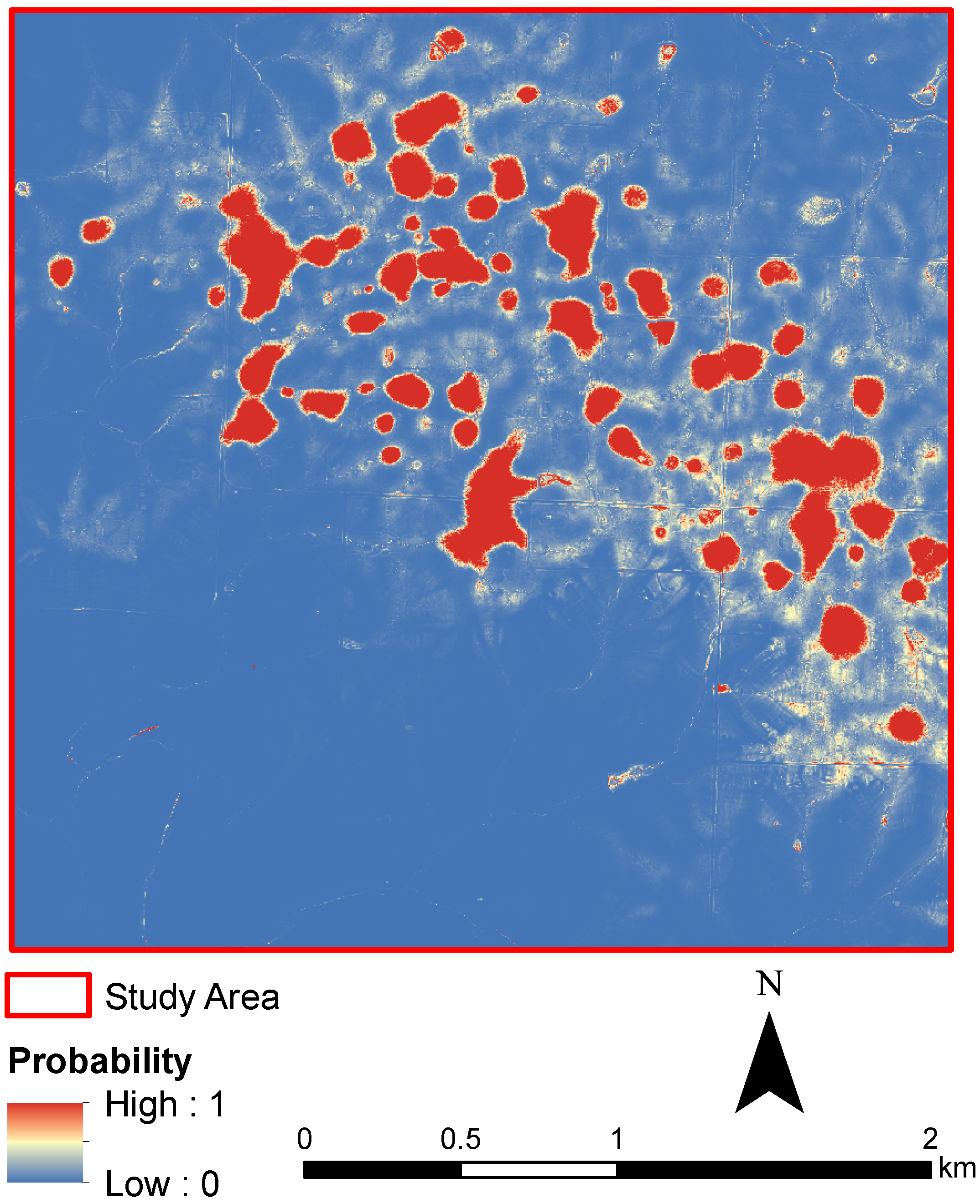
A positive coefficient tends to increase the probability of occurrence while a negative one implies the opposite outcome. Five independent variables, DEM, plan curvature, valley depth, MBI and TWI, exhibited a positive influence on sinkhole occurrence, while aspect, profile curvature, slope height, and MRVBF exerted a negative influence. Figure 5 shows the sinkhole susceptibility map created based on Equation (9); the computed probability of sinkhole occurrence varies from 0 to 1.

4.2. Cutoff Value

The resulting sinkhole susceptibility map (Figure 5) is a raster format in which each 1-m resolution grid cell represents the probability of sinkhole occurrence. In order to determine those high probability areas as sinkholes, a cutoff value was required. This cutoff threshold was determined based on the sensitivity and specificity tests. Sensitivity and specificity are statistical measures of the performance of a binary classification model [56]. The sensitivity (also known as a true positive rate) measures the proportion of actual positives that are correctly identified as such; thus, in this study, it tells how well the model detects sinkholes. The specificity (also known as a true negative rate) measures the proportion of negatives identified as such, and it tells how accurately the model avoids false sinkhole detections. The sensitivity and specificity were calculated as follows:
S e n s i t i v i t y = T P T P + F N
S p e c i f i c i t y = T N T N + F P
where TP is the number of true positives, FN is the number of false negatives, TN is the number of true negatives, and FP is the number of false positives.
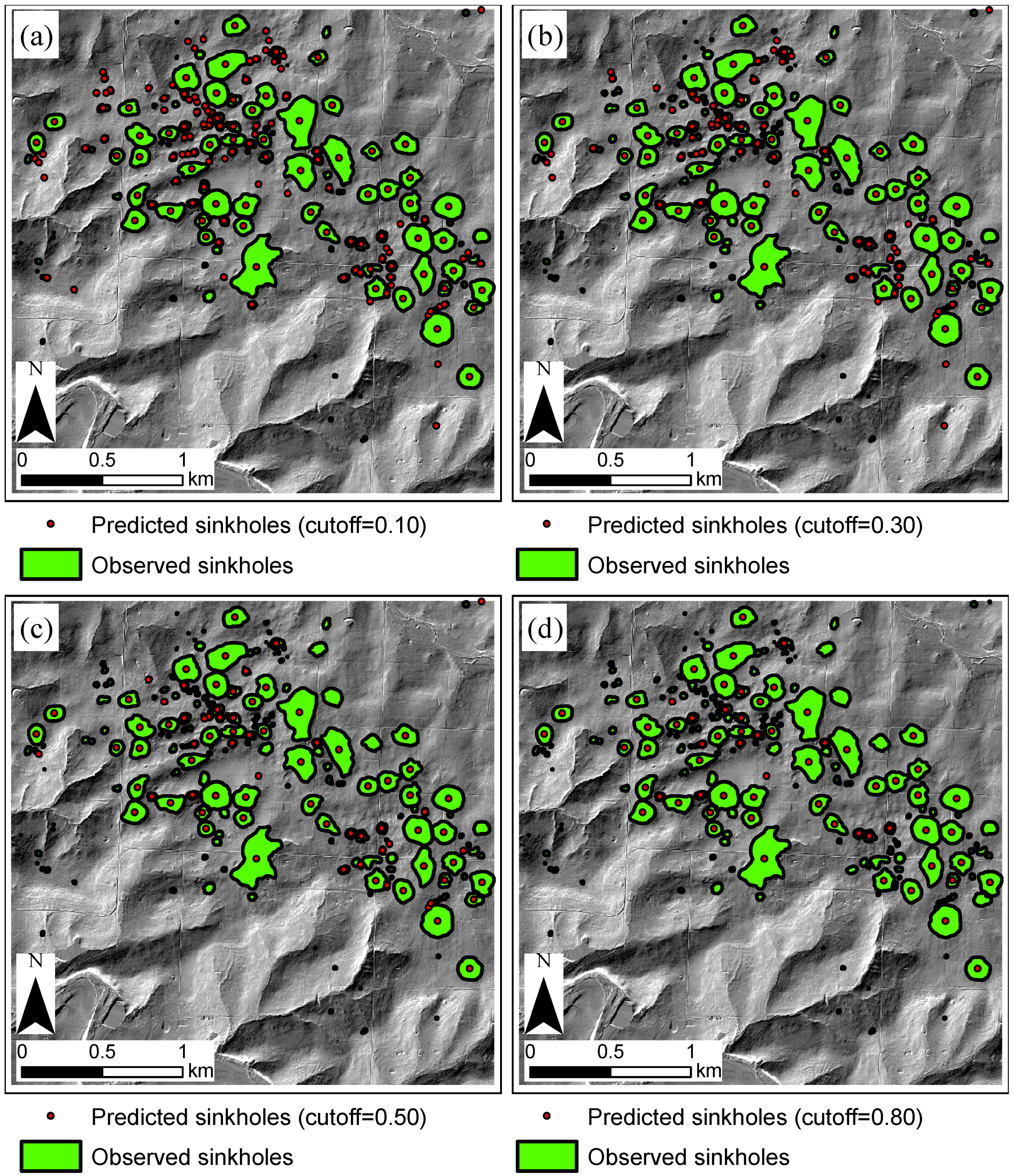
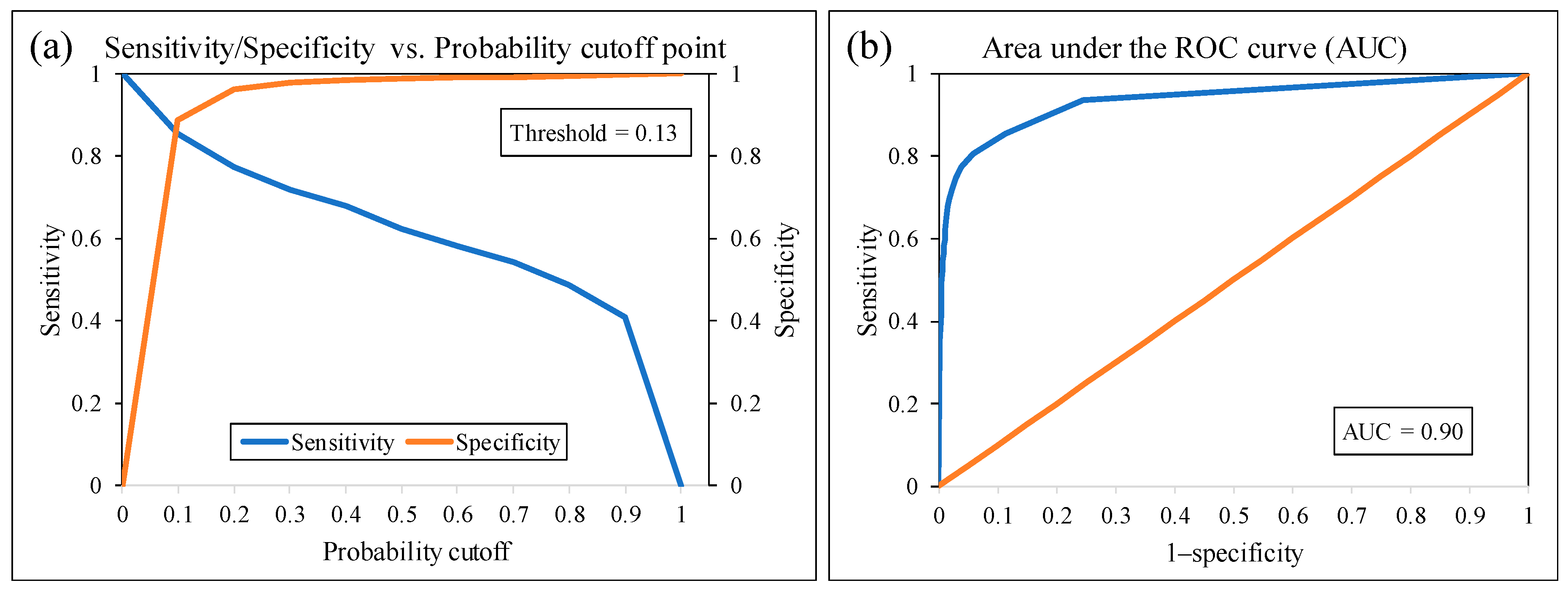
The setting of sensitivity and specificity is always a trade-off. If the cutoff value is set too low, the number of false negatives decreases, resulting in increased sensitivity. However, the number of false positives increases, and this results in decreased specificity. The effects changes in cutoff values on sinkhole identification are presented in Figure 6. The cutoff value varied from 0.1 to 0.8, and the sinkholes detected by the model were compared with the validated sinkhole database. In Figure 6a, the cutoff value was set low at 0.1 and the result shows a larger proportion of false positive results, leading to a decrease in true negative rate. In contrast, when the cutoff value was set high at 0.8 (Figure 6d), the number of true positives decreased. Thus, the optimum cutoff value of the model can be determined by maximizing the sum of sensitivity and specificity. For this study, the optimal cutoff value was determined as 0.13, which corresponds to the cross-point of sensitivity and specificity curves (Figure 7a). Figure 7b shows the area under the receiver operating characteristic (ROC) curve (also called the AUC). It is a plot of sensitivity versus 1–specificity for all possible cutoff classification probability values, showing the performance of a classification model at all possible probability values. In this study, the AUC was 0.90, demonstrating that the fitted LR model was highly reliable in explaining variability in sinkhole occurrence as a function of selected geomorphometric variables.

4.3. Sinkhole Susceptibility Map (Cutoff = 0.13)

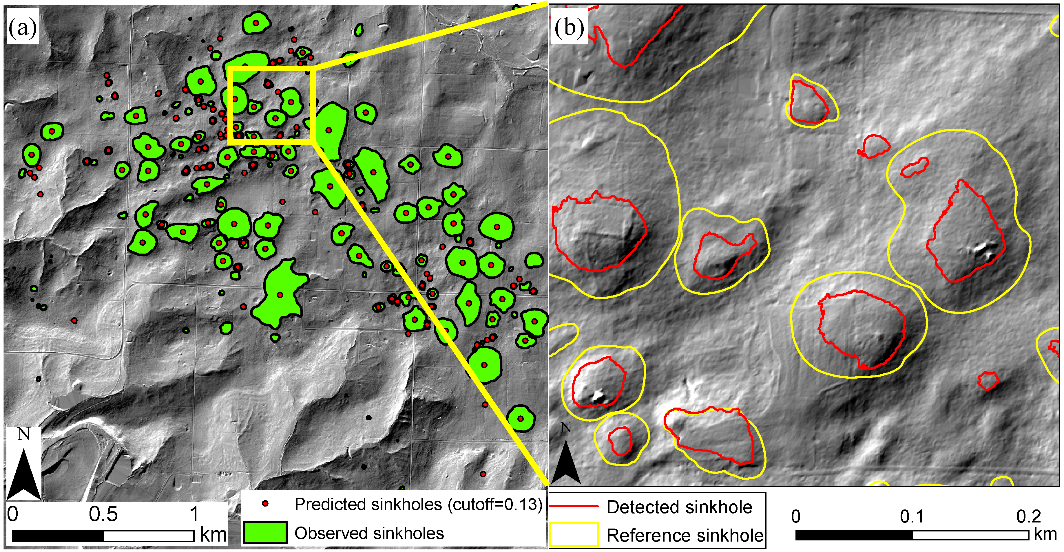
A new sinkhole map was developed in binary classification format using a cutoff value of 0.13 (Figure 8a). The map is a binary raster in which a value of 1 was assigned to grid cells with a probability of equal or greater than 0.13 and a value of 0 was assigned to any cell with a probability of less than 0.13. To produce sinkhole boundaries, contour lines were drawn by connecting all outer points of equal probability class. Figure 8b displays the sinkhole boundaries generated by the GLM model based on the selected cutoff value. Red and yellow lines represent the detected and reference sinkhole boundaries, respectively, in Figure 8b. This approach does not necessarily delineate the sinkhole boundaries but is able to locate sinkholes.
As previously discussed, more or wider sinkhole boundaries can be identified with application of a lower cutoff value. However, it also excessively identifies less susceptible areas for sinkholes and incurs unnecessary costs and time loss in sinkhole prevention and management. In contrast, too high a cutoff value can lead to low detection performance and high rates of false negatives. From the hazard management point of view, this scenario tends to be more dangerous. The damage from not knowing that the area has very high sinkhole potential would be more severe than believing falsely that the area has high potential of sinkholes. Therefore, it is recommended that a low cutoff value is used to minimize false negatives, i.e., avoid predicting an area as safe when it is actually dangerous.

4.4. Sinkhole Geometric Characterization

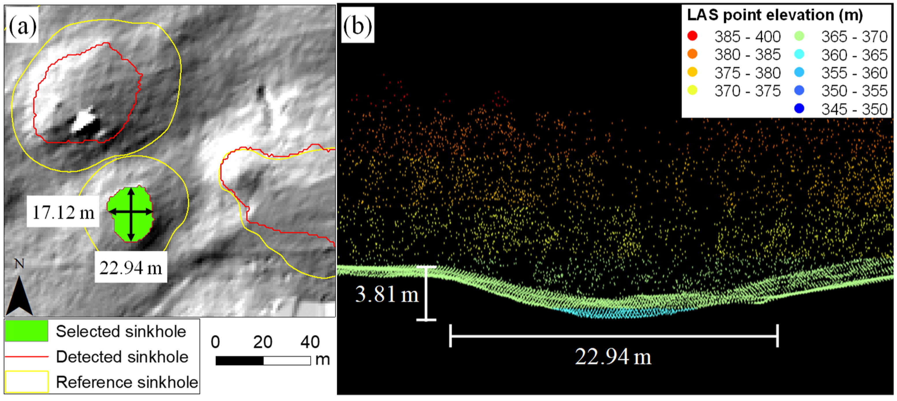
After sinkholes were detected, they were quantitatively evaluated regarding their geometric characteristics. Geometric characteristics of sinkholes include length, width, depth, perimeter, area, volume, elongatedness, and circularity. Length and width were defined as the lengths of the major and minor axes of the sinkhole, respectively. Depth is the maximum vertical distance from the lowest point within the sinkhole to the highest point of the sinkhole. Perimeter (or circumference) is the length around the outside of the sinkhole. Elongatedness can be calculated as the ratio of the length to width of the sinkhole. Sinkholes with elongatedness values close to 1 represent more circular shapes, while sinkholes with an elongated shape have higher elongatedness values. Circularity was defined as the ratio of the area of the shape to the area of a circle having the same perimeter and was measured as 4π × area/(perimeter)2. This is a measure of the degree of roundness of the sinkhole [57]. Sinkholes with a perfect circle have a value of 1, whereas a value less than 1 indicates an irregular shape. One sinkhole was selected as an example to determine geometric characteristics. Figure 9 shows the boundary of this sinkhole and a detailed 3D profile view of it, and Table 3 contains the summary of geometric characteristics of this sinkhole.

5. Conclusions

This study presents the sinkhole susceptibility map using LiDAR-derived DEM data. The following conclusions were drawn:
(1)
The sinkhole detection and characterization techniques were proposed using the LiDAR-derived DEM data. The proposed algorithm is believed to allow for improved consistency and repeatability.
(2)
Sixteen geomorphometric parameters were derived from DEM data, and a test for multicollinearity was conducted using both the Spearman correlation coefficient and VIF criteria. As a result, seven out of sixteen parameters were found to be highly correlated and were excluded in the further analyses. The selected nine parameters were DEM, aspect, plan curvature, profile curvature, slope height, valley depth, MRVBF, MBI, and TWI.
(3)
Logistic regression was used to construct the probabilistic sinkhole susceptibility map using the reported sinkhole inventory. In order to define the appropriate sinkhole boundaries from the probabilistic sinkhole susceptibility map, it is important to determine the optimal cutoff value. In this study, the recommended cutoff value was calculated to be 0.13, which has maximum sensitivity and specificity values at the same time.
(4)
The proposed sinkhole susceptibility map with the recommended cutoff value well predicted the reported sinkhole boundaries. While the model achieved a considerably high AUC of 0.90, the cutoff value is based on a training dataset of the study area, making the current results limited to the study area, and might not be applicable elsewhere.
(5)
Geometric features of sinkholes such as length, width, depth, perimeter, area, volume, elongatedness, and circularity can be estimated with the proposed sinkhole susceptibility map and LiDAR data.
(6)
Significant benefits of this study may include (1) identification of non-inventoried (e.g., newly formed or previously non-detected) sinkholes in the database, (2) automatic delineation of sinkhole boundaries, and (3) quantification of a sinkhole’s geometric characteristics.

Supplementary Materials

Supplementary materials are available online https://www.mdpi.com/2072-4292/11/13/1592/s1.

Author Contributions

B.H.N. conceived and designed the study; Y.J.K. interpreted and analyzed the LiDAR data; Y.J.K. and B.H.N prepared for the manuscript; B.H.N. and H.Y. provided a funding support; all authors contributed to discussion, revision, and editing.

Funding

National Research Foundation of Korea: 2016R1C1B2013478.

Acknowledgments

This work was supported by the National Research Foundation of Korea (NRF), funded by Ministry of Science, ICT & Future Planning (NRF-2016R1C1B2013478).

Conflicts of Interest

The authors declare no conflict of interest.

References

  1. Weary, D.J. The Cost of Karst Subsidence and Sinkhole Collapse in the United States Compared with Other Natural Hazards. In Proceedings of the 14th Multidisciplinary Conference on Sinkholes and the Engineering and Environmental Impacts of Karst, Rochester, MN, USA, 5–9 October 2015; pp. 433–446. [Google Scholar]
  2. Kuniansky, E.L.; Weary, D.J.; Kaufmann, J.E. The current status of mapping karst areas and availability of public sinkhole-risk resources in karst terrains of the United States. Hydrogeol. J. 2016, 24, 613–624. [Google Scholar] [CrossRef]
  3. Florida Office of Insurance Regulation. Report on Review of the 2010 Sinkhole Data Call. Available online: http://www.floir.com/siteDocuments/Sinkholes/2010_Sinkhole_Data_Call_Report.pdf (accessed on 3 July 2010).
  4. Gutiérrez, F.; Guerrero, J.; Lucha, P. A genetic classification of sinkholes illustrated from evaporite paleokarst exposures in Spain. Environ. Geol. 2008, 53, 993–1006. [Google Scholar] [CrossRef]
  5. Gutiérrez, F.; Parise, M.; De Waele, J.; Jourde, H. A review on natural and human-induced geohazards and impacts in karst. Earth Sci. Rev. 2014, 138, 61–88. [Google Scholar] [CrossRef]
  6. Ford, D.; Williams, P. Karst Hydrogeology and Geomorphology; John Wiley & Sons: New York, NY, USA, 2007; p. 562. [Google Scholar] [CrossRef]
  7. Williams, P.W. The role of the subcutaneous zone in karst hydrology. J. Hydrol. 1983, 61, 45–67. [Google Scholar] [CrossRef]
  8. Williams, P.W. Subcutaneous hydrology and the development of doline and cockpit karst. Z. Fur Geomorphol. 1985, 29, 463–482. [Google Scholar]
  9. Williams, P.W. Morphometric Analysis of Polygonal Karst in New Guinea. Geological. Soc. Am. Bull. 1972, 83, 761–796. [Google Scholar] [CrossRef]
  10. Lavalle, P. Some aspects of linear karst depression development in South Central Kentucky. Ann. Assoc. Am. Geogr. 1967, 57, 49–71. [Google Scholar] [CrossRef]
  11. Gutiérrez-Santolalla, F.; Gutiérrez-Elorza, M.; Marín, C.; Maldonado, C.; Younger, P.L. Subsidence hazard avoidance based on geomorphological mapping in the Ebro River valley mantled evaporite karst terrain (NE Spain). Environ. Geol. 2005, 48, 370–383. [Google Scholar] [CrossRef]
  12. Podobnikar, T.; Schöner, M.; Jansa, J.; Pfeifer, N. Spatial analysis of anthropogenic impact on karst geomorphology (Slovenia). Environ Geol. 2009, 58, 257–268. [Google Scholar] [CrossRef]
  13. Kobler, A.; Pfeifer, N.; Ogrinc, P.; Todorovski, L.; Oštir, K.; Džeroski, S. Repetitive interpolation: A robust algorithm for DTM generation from Aerial Laser Scanner Data in forested terrain. Remote Sens. Environ. 2007, 108, 9–23. [Google Scholar] [CrossRef]
  14. Hofton, M.A.; Rocchio, L.E.; Blair, J.B.; Dubayah, R. Validation of Vegetation Canopy Lidar sub-canopy topography measurements for a dense tropical forest. J. Geodyn. 2002, 34, 491–502. [Google Scholar] [CrossRef]
  15. Wu, Q.; Deng, C.; Chen, Z. Automated delineation of karst sinkholes from LiDAR-derived digital elevation models. Geomorphology 2016, 266, 1–10. [Google Scholar] [CrossRef]
  16. Gutiérrez, F.; Galve, J.P.; Lucha, P.; Castañeda, C.; Bonachea, J.; Guerrero, J. Integrating geomorphological mapping, trenching, InSAR and GPR for the identification and characterization of sinkholes: A review and application in the mantled evaporite karst of the Ebro Valley (NE Spain). Geomorphology 2011, 134, 144–156. [Google Scholar] [CrossRef] [Green Version]
  17. Filin, S.; Baruch, A.; Avni, Y.; Marco, S. Sinkhole characterization in the Dead Sea area using airborne laser scanning. Nat. Hazards 2011, 58, 1135–1154. [Google Scholar] [CrossRef]
  18. Kobal, M.; Bertoncelj, I.; Pirotti, F.; Dakskobler, I.; Kutnar, L. Using Lidar Data to Analyse Sinkhole Characteristics Relevant for Understory Vegetation under Forest Cover—Case Study of a High Karst Area in the Dinaric Mountains. PLoS ONE 2015, 10, e0122070. [Google Scholar] [CrossRef] [PubMed]
  19. Mukherjee, A.; Zachos, L.G. GIS Analysis of Sinkhole Distribution in Nixa, Missouri. In Proceedings of the GSA Annual Meeting & Exposition, Charlotte, NC, USA, 4–7 November 2012; p. 549. [Google Scholar]
  20. Zhu, J.; Taylor, T.P.; Currens, J.C.; Crawford, M.M. Improved Karst Sinkhole Mapping in Kentucky using LiDAR Techniques: A Pilot Study in Floyds Fork Watershed. J. Cave Karst Stud. 2014, 76, 207–216. [Google Scholar] [CrossRef]
  21. Obu, J.; Podobnikar, T. Algorithm for karst depression recognition using digital terrain models. Geod. Vestn. 2013, 57, 260–270. [Google Scholar] [CrossRef]
  22. Rahimi, M.; Alexander, E.C., Jr. Locating Sinkholes in LiDAR Coverage of a Glacio-Fluvial Karst, Winona County, MN. In Proceedings of the 13th Multidisciplinary Conference on Sinkholes and the Engineering and Environmental Impacts of Karst, Carlsbad, New Mexico, 6–10 May 2013; pp. 469–480. [Google Scholar]
  23. Sarkar, T.; Mishra, M. Soil Erosion Susceptibility Mapping with the Application of Logistic Regression and Artificial Neural Network. J. Geovisualization Sp. Anal. 2018, 2, 8. [Google Scholar] [CrossRef]
  24. Mousavi, S.Z.; Kavian, A.; Soleimani, K.; Mousavi, S.R.; Shirzadi, A. GIS-based spatial prediction of landslide susceptibility using logistic regression model. Geomat. Naturals Hazards Risk 2011, 2, 33–50. [Google Scholar] [CrossRef]
  25. Shafapour Tehrany, M.; Shabani, F.; Neamah Jebur, M.; Hong, H.; Chen, W.; Xie, X. GIS-based spatial prediction of flood prone areas using standalone frequency ratio, logistic regression, weight of evidence and their ensemble techniques. Geomat. Naturals Hazards Risk 2017, 8, 1538–1561. [Google Scholar] [CrossRef]
  26. Junek, W.N.; Jones, L.W.; Woods, M.T. Use of Logistic Regression for Forecasting Short-Term Volcanic Activity. Algorithms 2012, 5, 330–363. [Google Scholar] [CrossRef]
  27. Kim, K.; Kim, J.; Kwak, T.-Y.; Chung, C.-K. Logistic regression model for sinkhole susceptibility due to damaged sewer pipes. Nat. Hazards 2018, 93, 765–785. [Google Scholar] [CrossRef]
  28. Lamelas, M.T.; Marinoni, O.; Hoppe, A.; de la Riva, J. Doline probability map using logistic regression and GIS technology in the central Ebro Basin (Spain). Environ. Geol. 2008, 54, 963–977. [Google Scholar] [CrossRef]
  29. Ozdemir, A. Sinkhole susceptibility mapping using logistic regression in Karapınar (Konya, Turkey). Bull. Eng. Geol. Environ. 2016, 75, 681–707. [Google Scholar] [CrossRef]
  30. Missouri Department of Natural Resources. Missouri Geological Survey. Available online: https://dnr.mo.gov/geology/geosrv/envgeo/sinkholes.htm (accessed on 8 April 2019).
  31. Missouri Spatial Data Information Service. Missouri LiDAR Data; LiDAR DEM Download Tool. Available online: http://msdis.missouri.edu/data/lidar/ (accessed on 27 March 2019).
  32. Greene County, Missouri; 2011 Digital Mapping Project; LiDAR & Survey Report; Greene County. Available online: ftp://lidar.wustl.edu/Greene/0196%20Greene_County_LiDAR_Final_Report.pdf (accessed on 3 July 2019).
  33. Conrad, O.; Bechtel, B.; Bock, M.; Dietrich, H.; Fischer, E.; Gerlitz, L.; Wehberg, J.; Wichmann, V.; Böhner, J. System for Automated Geoscientific Analyses (SAGA) v. 2.1.4. Geosci. Model Dev. 2015, 8, 1991–2007. [Google Scholar] [CrossRef] [Green Version]
  34. Zevenbergen, L.W.; Thorne, C.R. Quantitative analysis of land surface topography. Earth Surf. Proc. Landf. 1987, 12, 47–56. [Google Scholar] [CrossRef]
  35. Wilson, J.P.; Gallant, J.C. Primary Topographic Attributes. In Terrain Analysis: Principles and Applications; Wilson, J.P., Gallant, J.C., Eds.; John Wiley & Sons: Hoboken, NJ, USA, 2000; pp. 51–85. [Google Scholar]
  36. Xu, C.; Xu, X.; Dai, F.; Saraf, A.K. Comparison of different models for susceptibility mapping of earthquake triggered landslides related with the 2008 Wenchuan earthquake in China. Comput. Geosci. 2012, 46, 317–329. [Google Scholar] [CrossRef]
  37. Mancini, F.; Ceppi, C.; Ritrovato, G. GIS and statistical analysis for landslide susceptibility mapping in the Daunia area, Italy. Nat. Hazards Earth Syst. Sci. 2010, 10, 1851–1864. [Google Scholar] [CrossRef] [Green Version]
  38. Böhner, J.; Selige, T. Spatial Prediction of Soil Attributes Using Terrain Analysis and Climate Regionalization. Available online: https://www.researchgate.net/publication/267821689_Spatial_prediction_of_soil_attributes_using_terrain_analysis_and_climate_regionalization (accessed on 2 July 2019).
  39. Böhner, J.; Antonić, O. Chapter 8 Land-Surface Parameters Specific to Topo-Climatology. In Developments in Soil Science; Hengl, T., Reuter, H.I., Eds.; Elsevier: Amsterdam, The Netherlands, 2009; Volume 33, pp. 195–226. [Google Scholar]
  40. Köthe, R.; Lehmeier, F. SARA— System zur Automatischen Relief-Analyse, Benutzerhandbuch; Department of Geography, University of Göttingen: Göttingen, Germany, 1996; p. 24. [Google Scholar]
  41. Dietrich, H.; Böhner, J. Cold Air Production and Flow in a Low Mountain Range Landscape in Hessia (Germany). In SAGA–Seconds Out, Hamburger Beiträge zur Physischen Geographie und Landschaftsökologie; University Hamburg, Institut für Geographie: Hamburg, Germany, 2008; Volume 19, pp. 37–48. [Google Scholar]
  42. Gallant, J.C.; Dowling, T.I. A multiresolution index of valley bottom flatness for mapping depositional areas. Water Res. Res. 2003, 39. [Google Scholar] [CrossRef]
  43. Möller, M.; Volk, M.; Friedrich, K.; Lymburner, L. Placing soil-genesis and transport processes into a landscape context: A multiscale terrain-analysis approach. J. Plant Nutr. Soil Sci. 2008, 171, 419–430. [Google Scholar] [CrossRef]
  44. Guisan, A.; Weiss, S.B.; Weiss, A.D. GLM versus CCA spatial modeling of plant species distribution. Plant Ecol. 1999, 143, 107–122. [Google Scholar] [CrossRef]
  45. Beven, K.J.; Kirkby, M.J. A physically based, variable contributing area model of basin hydrology Un modèle à base physique de zone d’appel variable de l’hydrologie du bassin versant. Hydrol. Sci. Bull. 1979, 24, 43–69. [Google Scholar] [CrossRef]
  46. Guisan, A.; Edwards, T.C.; Hastie, T. Generalized linear and generalized additive models in studies of species distributions: Setting the scene. Ecol. Modellier 2002, 157, 89–100. [Google Scholar] [CrossRef]
  47. Franklin, J. Mapping Species Distributions: Spatial Inference and Prediction; Cambridge University Press: Cambridge, UK, 2010. [Google Scholar] [CrossRef]
  48. Myers, R.H.; Montgomery, D.; Vining, G.G.; Robinson, T.J. Generalized Linear Models: With Applications in Engineering and the Sciences, 2nd ed.; John Wiley and Sons Inc.: New York, NY, USA, 2012. [Google Scholar] [CrossRef]
  49. Hosmer, D.W.; Jovanovic, B.; Lemeshow, S. Best Subsets Logistic Regression. Biometrics 1989, 45, 1265–1270. [Google Scholar] [CrossRef]
  50. Schwarz, G. Estimating the Dimension of a Model. Ann. Stat. 1978, 6, 461–464. [Google Scholar] [CrossRef]
  51. Akaike, H. A new look at the statistical model identification. IEEE Trans. Autom. Control. 1974, 19, 716–723. [Google Scholar] [CrossRef]
  52. Field, A. Discovering Statistics Using SPSS, 2nd ed.; Sage Publications, Inc.: Thousand Oaks, CA, USA, 2005; p. xxxiv, 779. [Google Scholar]
  53. Quinn, G.P.; Keough, M.J. Experimental Design and Data Analysis for Biologists; Cambridge University Press: Cambridge, UK, 2002. [Google Scholar] [CrossRef]
  54. Hair, J.F., Jr.; Black, W.C.; Babin, B.J.; Anderson, R.E. Multivariate Data Analysis, 7th ed.; Prentice-Hall: Upper Saddle River, NJ, USA, 2010. [Google Scholar]
  55. Hosmer, D.W., Jr.; Lemeshow, S.; Sturdivant, R.X. Applied Logistic Regression, 3rd ed.; John Wiley & Sons, Inc.: Hoboken, NJ, USA, 2013; Volume 398, p. 528. [Google Scholar]
  56. Altman, D.G.; Bland, J.M. Diagnostic tests. 1: Sensitivity and specificity. BMJ 1994, 308, 1552. [Google Scholar] [CrossRef] [PubMed]
  57. Pratt, W.K. Digital Image Processing: PIKS Scientific Inside, 4th ed.; John Wiley & Sons, Inc.: New York, NY, USA, 2006. [Google Scholar]
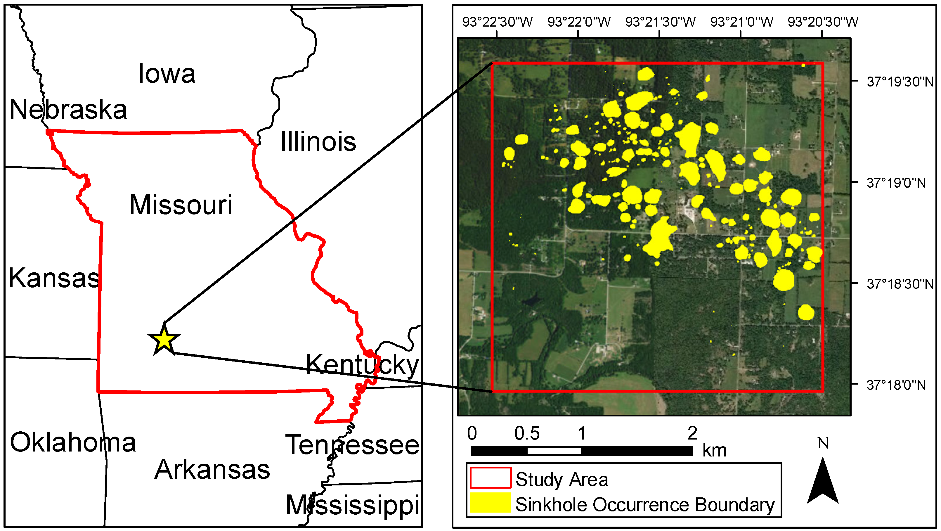
Figure 1. Location of study area and sinkhole occurrence boundary (Missouri, USA).
Remotesensing 11 01592 g001
Figure 2. Flow chart of the study.
Remotesensing 11 01592 g002
Figure 3. Geomorphometric indices of the study area used for the final model: (a) DEM; (b) aspect; (c) PLC; (d) PRC; (e) SH; (f) VD; (g) MRVBF; (h) MBI; and (i) TWI.
Remotesensing 11 01592 g003
Figure 4. Summary of Spearman correlation coefficient analysis of geomorphometric indices.
Remotesensing 11 01592 g004
Figure 5. Probabilistic sinkhole susceptibility map of the study area using LR method.
Remotesensing 11 01592 g005
Figure 6. Effect of cutoff value on sensitivity and specificity of test results when cutoff value is: (a) 0.1; (b) 0.3; (c) 0.5; and (d) 0.8.
Remotesensing 11 01592 g006
Figure 7. Plot of (a) sensitivity and specificity versus probability cutoff value; and (b) area under the receiver operating characteristic (ROC) curve.
Remotesensing 11 01592 g007
Figure 8. Map of (a) sinkhole susceptibility with cutoff of 0.13; and (b) reference sinkholes (yellow) and detected sinkholes by GLM model (red).
Remotesensing 11 01592 g008
Figure 9. Geometric characteristics: (a) Aerial image and sinkhole boundaries; and (b) 3D profile view of selected sinkhole.
Remotesensing 11 01592 g009
Table 1. Coefficients of the logistic regression for sinkhole prediction models.
ModelVariableEstimateStd. ErrorWald Statisticp Value
1(Intercept)−42.33000.0825−513.36<0.001
DEM0.10490.0002477.55<0.001
Aspect−0.00060.0000−45.16<0.001
PLC20.97000.1549135.37<0.001
PRC−5.57400.1141−48.87<0.001
SH−0.60340.0016−385.24<0.001
VD0.09480.001095.37<0.001
MSP0.01600.00533.030.00245
MRVBF−0.72960.0019−384.52<0.001
MBI0.33630.0020170.92<0.001
TWI0.55540.0006900.12<0.001
2(Intercept)−42.30000.0817−517.79<0.001
DEM0.10490.0002480.31<0.001
Aspect−0.00060.0000−45.15<0.001
PLC20.97000.1549135.39<0.001
PRC−5.56700.1140−48.81<0.001
SH−0.60380.0016−386.81<0.001
VD0.09520.001096.62<0.001
MRVBF−0.72890.0019−387.56<0.001
MBI0.33630.0020170.92<0.001
TWI0.55530.0006900.45<0.001
3(Intercept)−42.40000.0817−519.16<0.001
DEM0.10490.0002480.30<0.001
PLC21.05000.1549135.94<0.001
PRC−5.62400.1141−49.29<0.001
SH−0.60600.0016−388.74<0.001
VD0.09320.001094.45<0.001
MRVBF−0.72890.0019−387.56<0.001
MBI0.33620.0020170.92<0.001
TWI0.55550.0006900.74<0.001
Note: Estimate: The regression coefficient that explains the change in log(odds) of the dependent variable for one unit change in the independent variable; Std. error: The standard errors of estimated coefficients; Wald statistic: The regression coefficient divided by standard error; p value: The significance probability of independent variables.
Table 2. LR models fit statistics.
Model 1Model 2Model 3
Measures of fitAIC3,788,5663,788,5743,790,610
BIC3,788,7213,788,7143,790,736
Pseudo R20.6910.6920.692
Table 3. Results of sinkhole geometric characteristics.
Length
(m)
Width
(m)
Depth
(m)
Perimeter
(m)
Area
(m2)
Volume
(m3)
ElongatednessCircularity
22.9417.123.8163.26308.45852.941.340.97