A Review of Techniques for Diagnosing the Atmospheric Boundary Layer Height (ABLH) Using Aerosol Lidar Data


Abstract
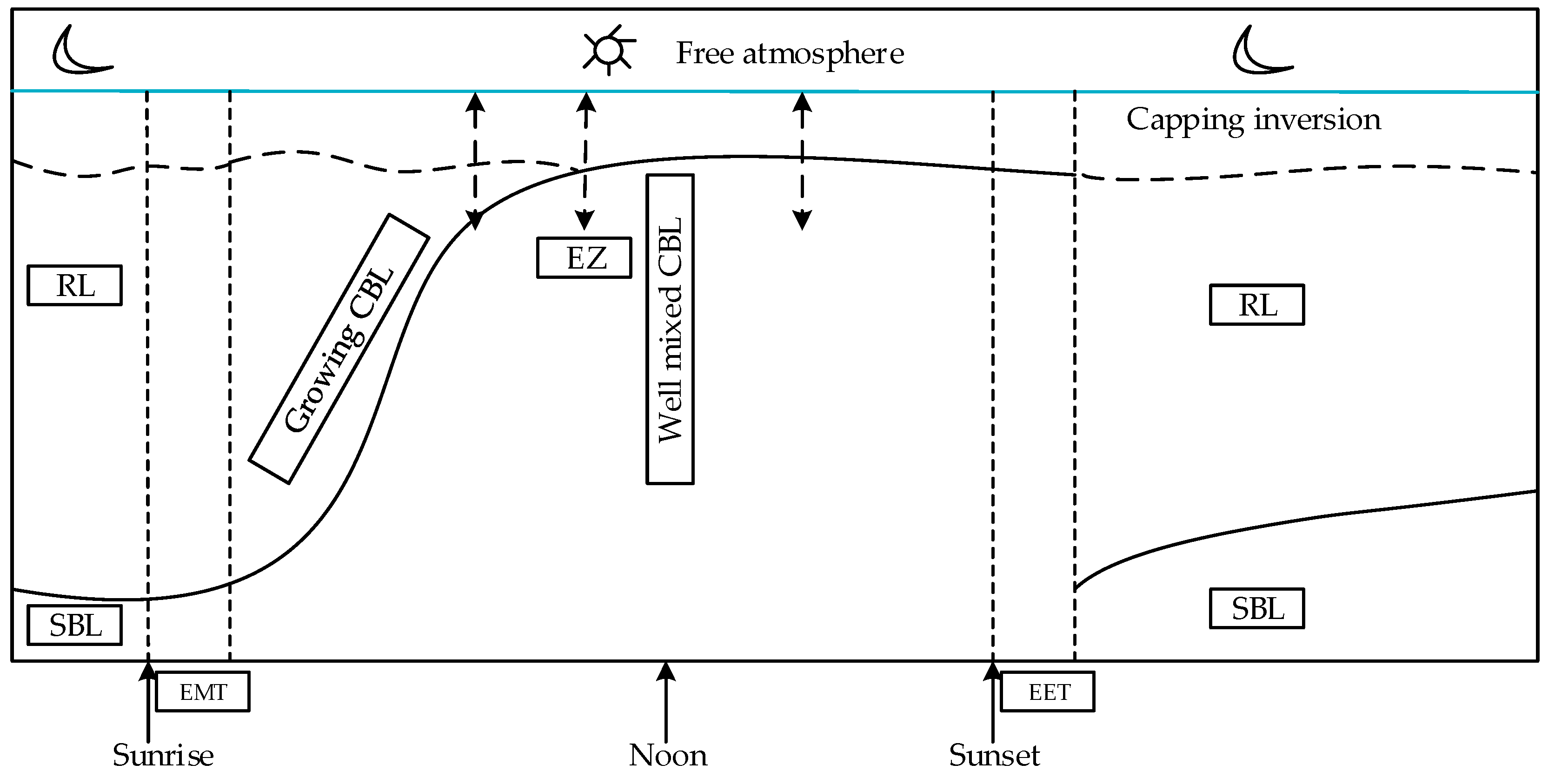
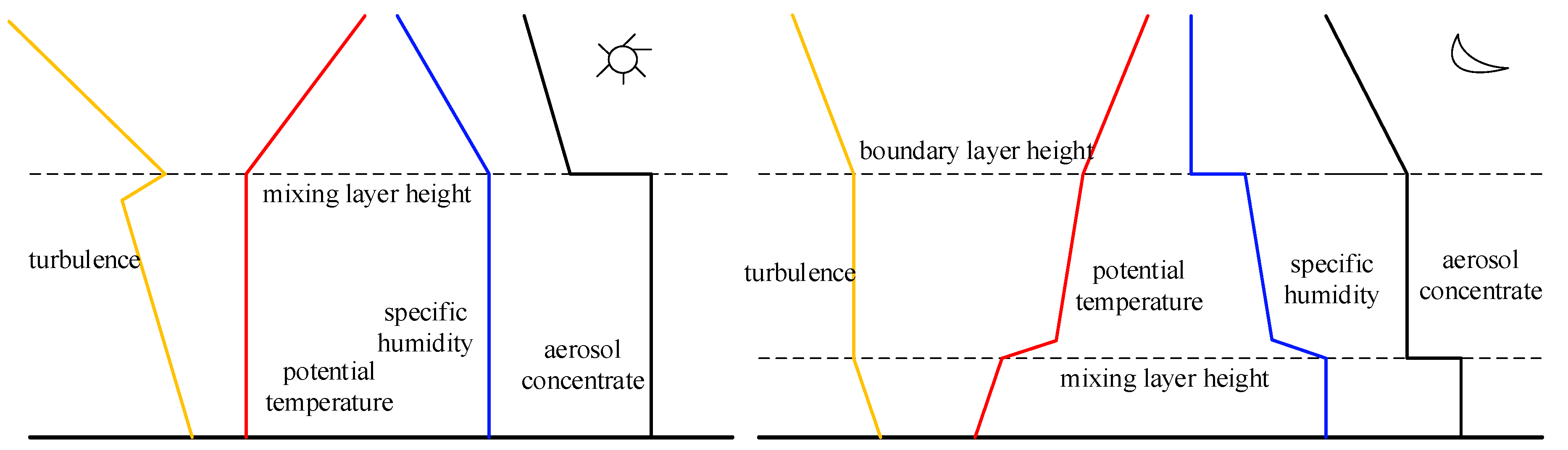
1. Introduction
2. Classical Methodologies for Lidar Measurement of ABLH
2.1. Visual Inspection (or Ocular Estimate)
2.2. Thereshold Method
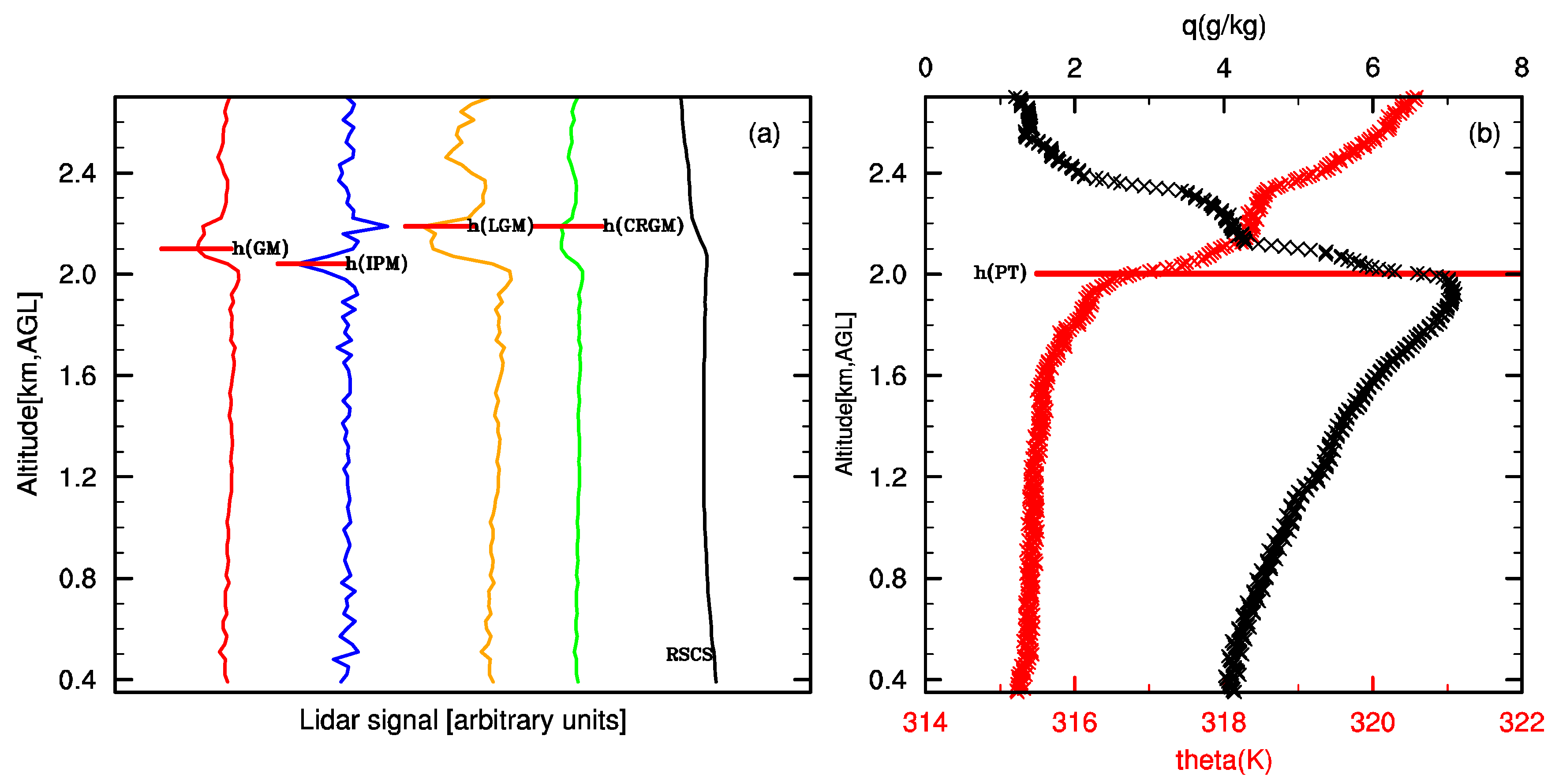
2.3. Gradient Method (GMs)
2.4. Ideal Profile Fitting (Curve Fitting) (FIT)
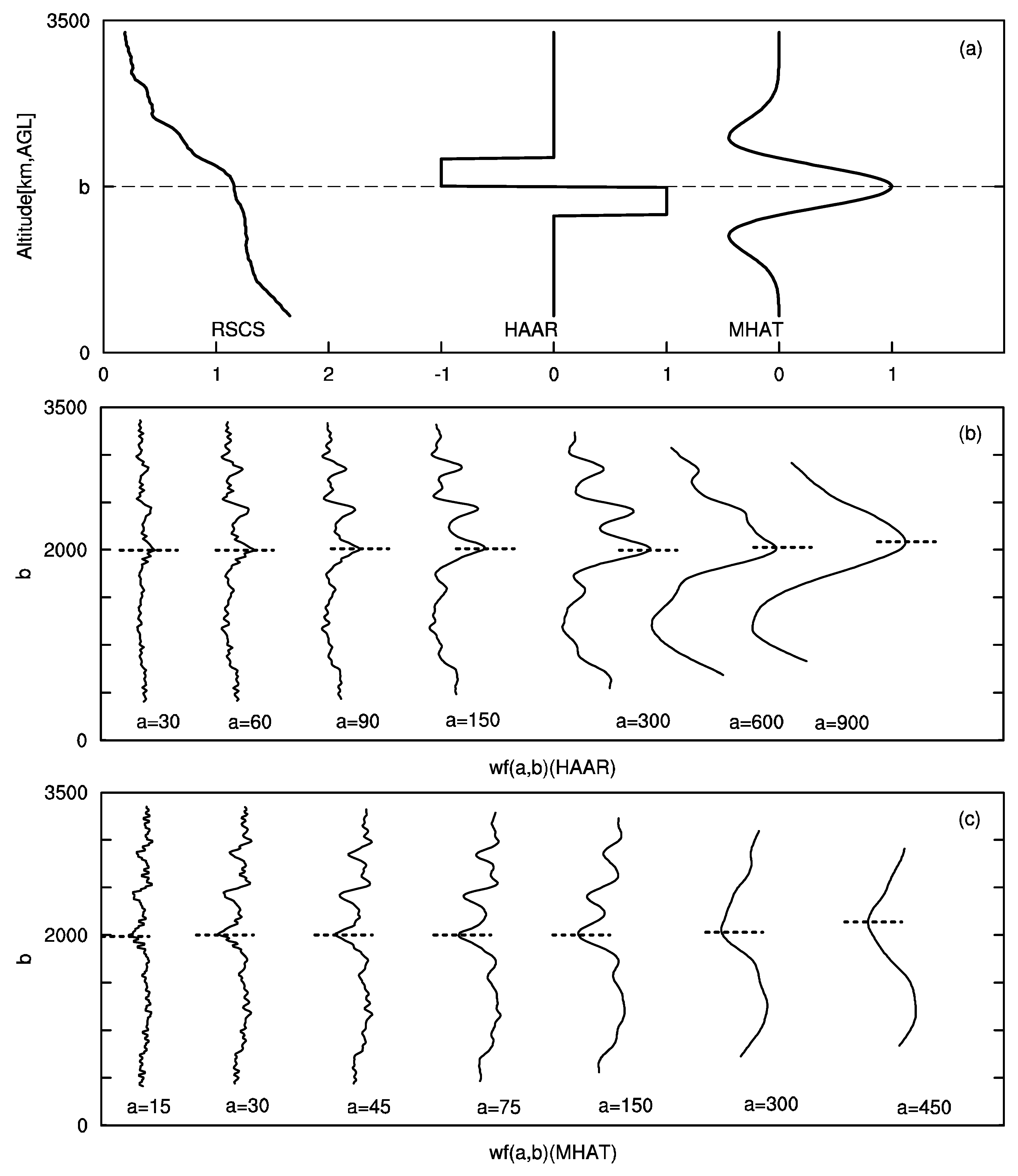
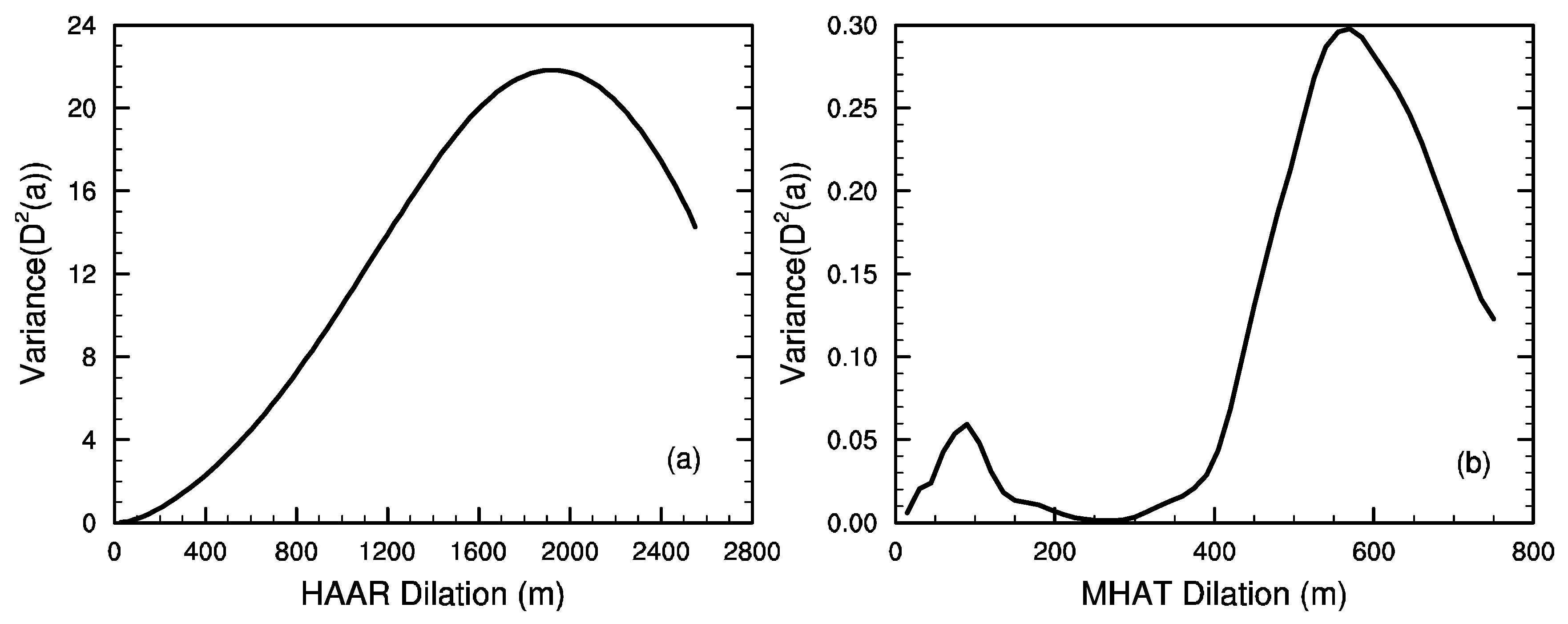
2.5. Wavelet Covariance Transform (WCT)
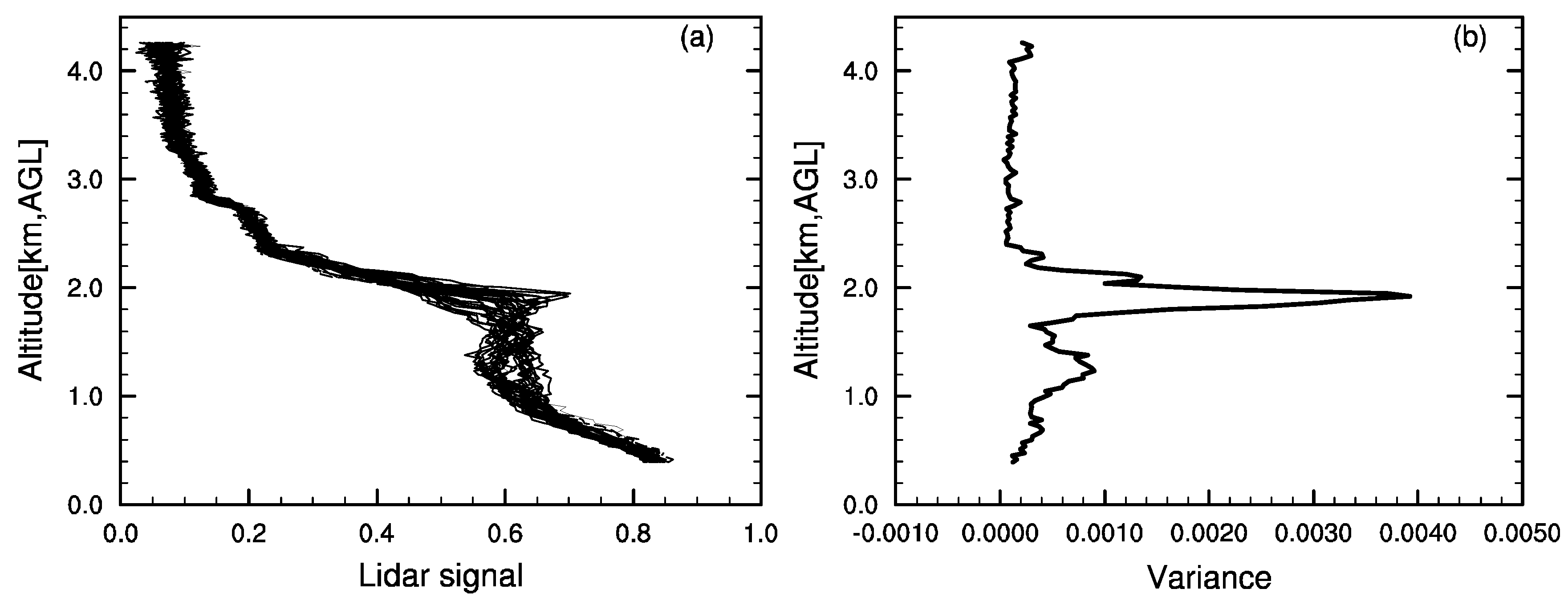
2.6. Variance (or Standard Deviation) Analysis (VAR or STD)
3. Improvement of Some Classical Methodologies
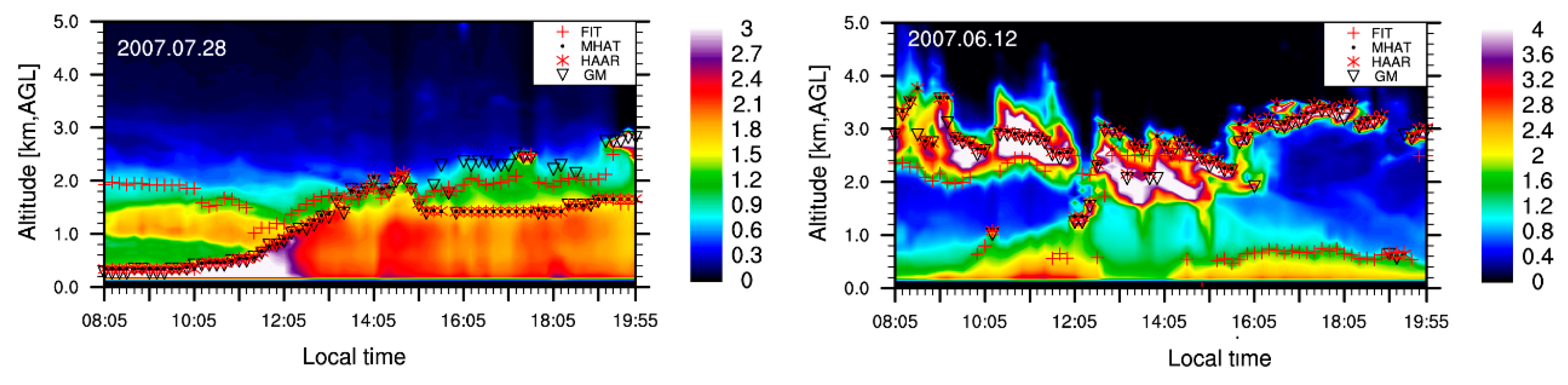
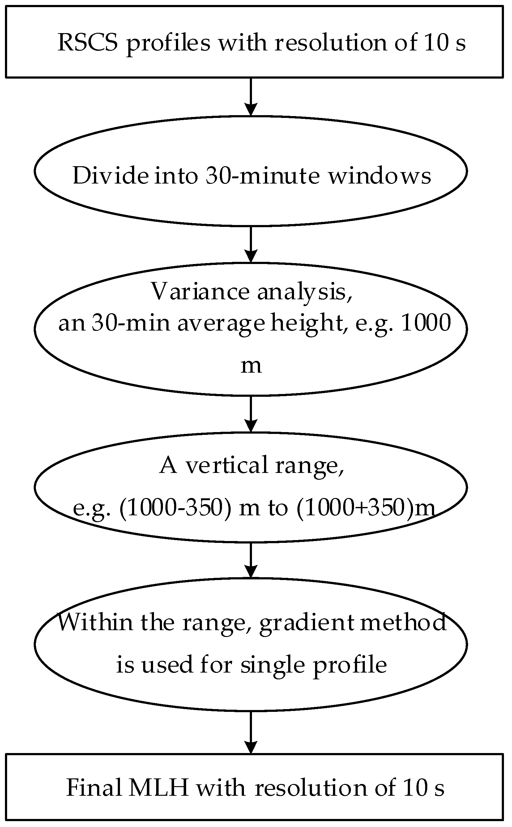
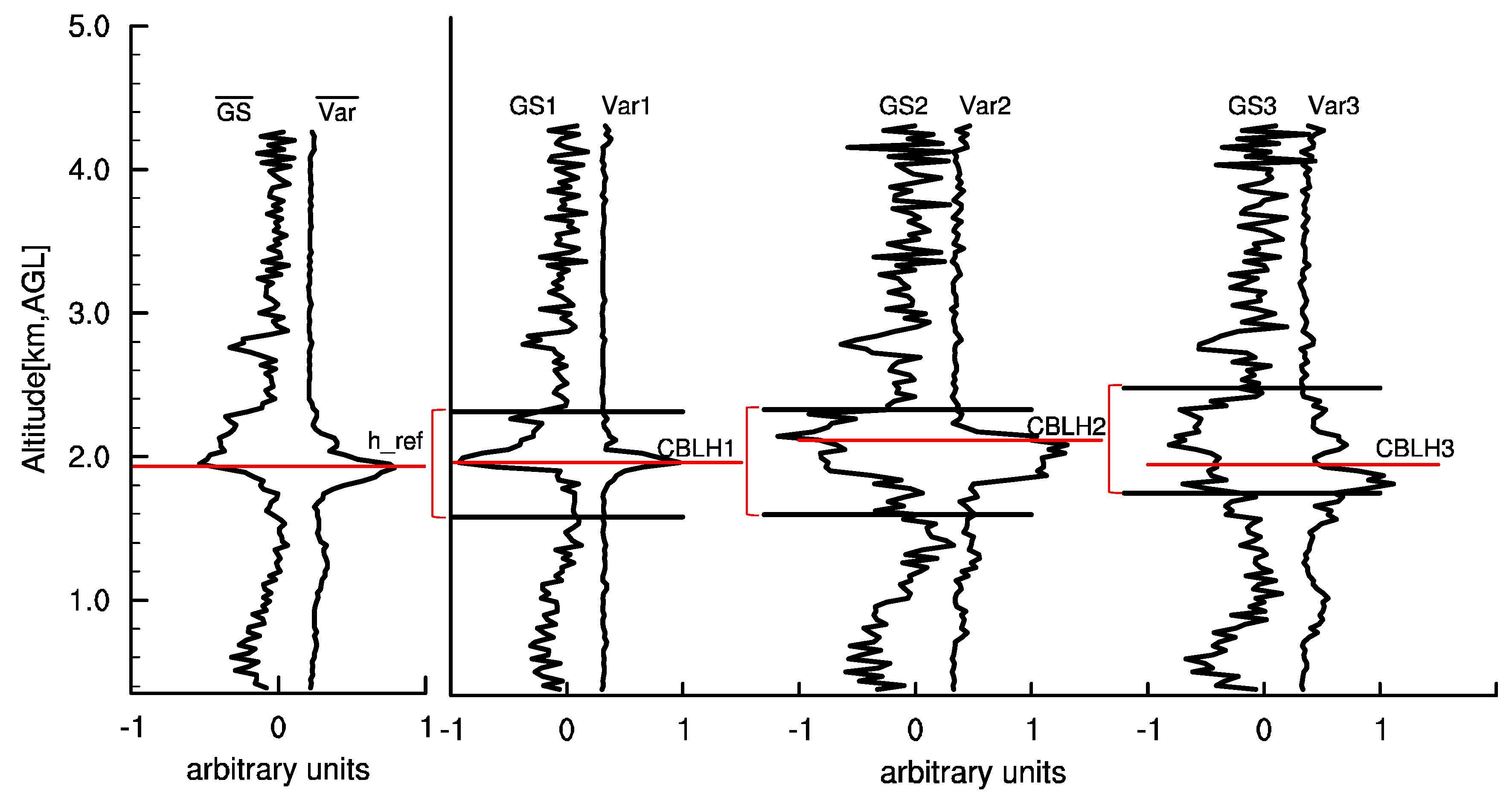
3.1. The Combination of GM and VAR
- For RSCS profile with time resolution of 60 s, the single and profiles provide single evaluations of the MLH (for 1.5 h measurement, goes from 1 to 90), the moving variance analysis is applied to each -profile within the temporal interval ,.
- An average signal gradient profile and a variance profile are calculated over a time interval of 30 min, named and . The reference height () is defined as the middle position of the heights of the minimum and the maximum, the related error is , where the standard deviations of and are calculated over the 30 min average at .
- For , within a vertical range , is determined as the middle position of the local minimum of and local maximum of the .
- For , within the vertical range , the is determined as the middle position of the local minimum of and local maximum of the . For next time window (), procedures 2 to–4 are repeated, a simple scheme for THT algorithm is shown as Figure 10.
3.2. The Combination of Thereshold Method and WCT
3.3. The Combination of FIT and WCT
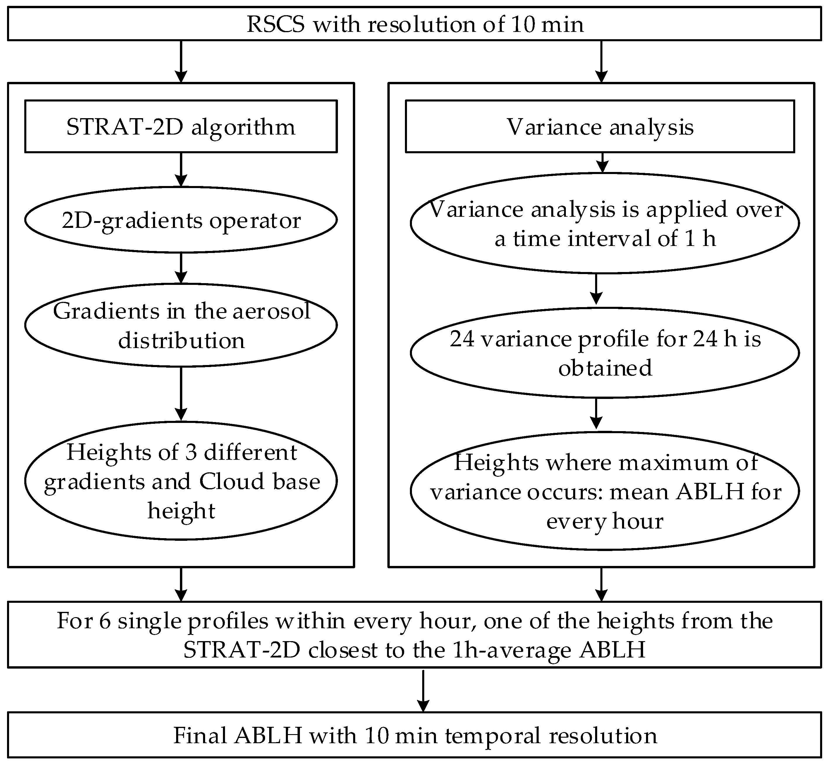
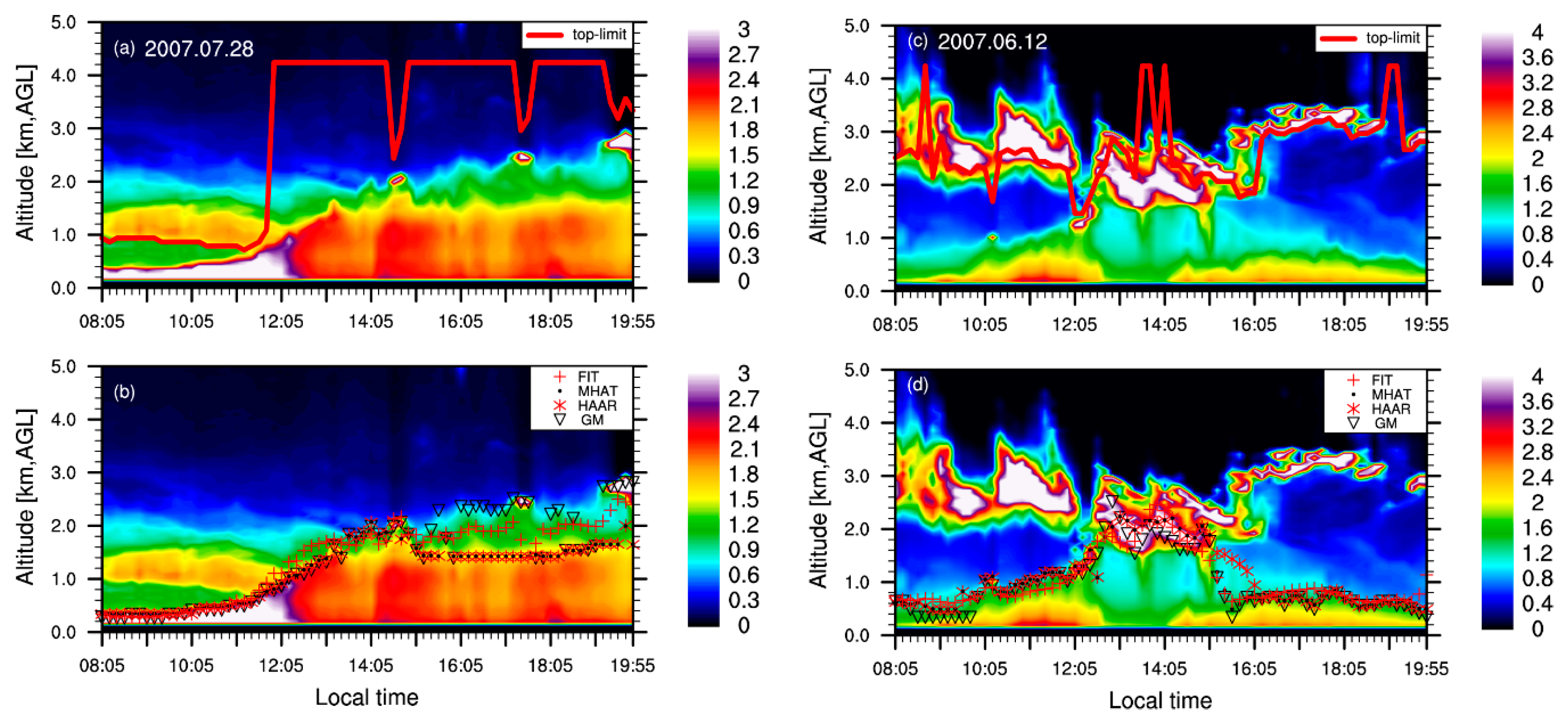
3.4. 2D Version of Structure of the Atmosphere (STRAT-2D)
3.5. Height Restriction for Some Classical Methodologies
4. New Techniques Developed Recently
4.1. New Techniques Based on Single-Wavelength Lidar
4.2. ABLH Determination from Multi-Walelength Lidar
5. Summary and Conclusions
Author Contributions
Funding
Acknowledgments
Conflicts of Interest
References
- Stull, R.B. An introduction to boundary layer meteorology. In Atmospheric Sciences Library; Springer: Berlin, Germany, 1988; Volume 8, p. 89. [Google Scholar]
- Seibert, P.; Beyrich, F.; Gryning, S.-E.; Joffre, S.; Rasmussen, A.; Tercier, P. Review and intercomparison of operational methods for the determination of the mixing height. Atmos. Environ. 2000, 34, 1001–1027. [Google Scholar] [CrossRef]
- Garratt, J.R. The Atmospheric Boundary Layer; Cambridge University Press: Cambridge, UK, 1992. [Google Scholar]
- Beyrich, F.; Gryning, S.E.; Joffre, S.; Rasmussen, A.; Seibert, P.; Tercier, P. Mixing Height Determination for Dispersion Modelling—A Test of Meteorological Pre-Processors. In Air Pollution Modeling and Its Application XII.; Springer: Boston, USA, 1998. [Google Scholar]
- Haman, C.L.; Lefer, B.; Morris, G.A. Seasonal variability in the diurnal evolution of the boundary layer in a near-coastal urban environment. J. Atmos. Ocean. Technol. 2012, 29, 697–710. [Google Scholar] [CrossRef]
- Granados-Muñoz, M.J.; Navas-Guzmán, F.; Bravo-Aranda, J.A.; Guerrero-Rascado, J.L.; Lyamani, H.; Fernández-Gálvez, J.; Alados-Arboledas, L. Automatic determination of the planetary boundary layer height using lidar: One-year analysis over southeastern Spain. J. Geophys. Res. Atmos. 2012, 117. [Google Scholar] [CrossRef]
- Pal, S.; Haeffelin, M.; Batchvarova, E. Exploring a geophysical process-based attribution technique for the determination of the atmospheric boundary layer depth using aerosol lidar and near-surface meteorological measurements. J. Geophys. Res.-Atmos. 2013, 118, 9277–9295. [Google Scholar] [CrossRef]
- Seibert, P.; Beyrich, F.; Gryning, S.E.; Joffre, S.; Rasmussen, A.; Tercier, P. Mixing height determination for dispersion modeling, Report of Working Group 2. In Harmonization in the Preprocessing of Meteorological Data for Atmospheric Dispersion Models. COST Action 710. Final Report; Office for official Publications of the European Communities: Luxembourg, 1998. [Google Scholar]
- Cooper, D.I.; Eichinger, W.E. Structure of the atmosphere in an urban planetary boundary layer from lidar and radiosonde observations. J. Geophys. Res. Atmos. 1994, 99, 22937–22948. [Google Scholar] [CrossRef]
- Seidel, D.J.; Ao, C.O.; Li, K. Estimating climatological planetary boundary layer heights from radiosonde observations: Comparison of methods and uncertainty analysis. J. Geophys. Res. Atmos. 2010, 115. [Google Scholar] [CrossRef]
- Jeričević, A.; Kraljević, L.; Grisogono, B.; Fagerli, H.; Večenaj, Ž. Parameterization of vertical diffusion and the atmospheric boundary layer height determination in the EMEP model. Atmos. Chem. Phys. 2010, 10, 341–364. [Google Scholar] [CrossRef]
- Norton, C.L.; Hoidale, G.B. The diurnal variation of mixing height by month over White Sands Missile Range, New Mexico. Mon. Weather Rev. 1976, 104, 1317–1320. [Google Scholar] [CrossRef]
- Wang, X.; Wang, K. Homogenized Variability of Radiosonde Derived Atmospheric Boundary Layer Height over the Global Land Surface from 1973 to 2014. J. Clim. 2016, 29, 6893–6908. [Google Scholar] [CrossRef]
- Basha, G.; Kishore, P.; Ratnam, M.V.; Babu, S.R.; Velicogna, I.; Jiang, J.H.; Ao, C.O. Global climatology of planetary boundary layer top obtained from multi-satellite GPS RO observations. Clim. Dyn. 2019, 52, 2385–2398. [Google Scholar] [CrossRef]
- Seidel, D.J.; Zhang, Y.; Beljaars, A.C.M.; Golaz, J.C.; Jabobson, A.R.; Medeiros, B. Climatology of the planetary boundary layer over the continental United States and Europe. J. Geophys. Res. Atmos. 2012, 117. [Google Scholar] [CrossRef]
- Guo, J.; Miao, Y.; Zhang, Y.; Liu, H.; Li, Z.; Zhang, W.; He, J.; Lou, M.; Yan, Y.; Bian, L. The climatology of planetary boundary layer height in China derived from radiosonde and reanalysis data. Atmos. Chem. Phys. 2016, 16, 13309–13319. [Google Scholar] [CrossRef]
- Moores, W.H.; Caughey, S.J.; Readings, C.J.; Milford, J.R.; Mansfield, D.A.; Abdulla, S.; Guymer, T.H.; Johnston, W.B. Measurements of boundary layer structure and development over SE England using aircraft and tethered balloon instrumentation. Q. J. R. Meteorol. Soc. 1979, 105, 397–421. [Google Scholar] [CrossRef]
- Jordi, V.G.d.A.; Duynkerke, P.G.; Weele, M.V. Tethered-balloon measurements of actinic flux in a cloud-capped marine boundary layer. J. Geophys. Res. Atmos. 1994, 99, 3699–3706. [Google Scholar]
- Holden, J.J.; Derbyshire, S.H.; Belcher, S.E. Tethered Balloon Observations of the Nocturnal Stable Boundary Layer in a Valley. Bound.-Layer Meteorol. 2000, 97, 1–24. [Google Scholar] [CrossRef]
- Vernekar, K.G.; Sadani, L.K.; Brij, M.; Saxena, S.; Debaje, S.B.; Pillai, J.S.; Murthy, B.S.; Patil, M.N. Structure and growth of atmospheric boundary layer as observed by a tethered balloon payload. Indian J. Radio Space Phys. 1991, 20, 312–315. [Google Scholar]
- Dai, C.Y.; Gao, Z.Q.; Wang, Q.; Cheng, G. Analysis of Atmospheric Boundary Layer Height Characteristics over the Arctic Ocean Using the Aircraft and GPS Soundings. Atmos. Ocean. Sci. Lett. 2011, 4, 124–130. [Google Scholar]
- Dai, C.; Wang, Q.; Kalogiros, J.A.; Lenschow, D.H.; Gao, Z.; Zhou, M. Determining Boundary-Layer Height from Aircraft Measurements. Bound.-Layer Meteorol. 2014, 152, 277–302. [Google Scholar] [CrossRef]
- Galmarini, S.; Attié, J.L. Turbulent Transport atthe Thermal Internal Boundary-Layer top: Wavelet Analysis of Aircraft Measurements. Bound.-Layer Meteorol. 2000, 94, 175–196. [Google Scholar] [CrossRef]
- Beyrich, F. On the use of SODAR data to estimate mixing height. Appl. Phys. B Photophys. Laser Chem. 1993, 57, 27–35. [Google Scholar] [CrossRef]
- Beyrich, F.; Weill, A. Some aspects of determining the stable boundary layer depth from sodar data. Bound.-Layer Meteorol. 1993, 63, 97–116. [Google Scholar] [CrossRef]
- Emeis, S.; Münkel, C.; Vogt, S.; Müller, W.J.; Schäfer, K. Atmospheric boundary-layer structure from simultaneous SODAR, RASS, and ceilometer measurements. Atmos. Environ. 2004, 38, 273–286. [Google Scholar] [CrossRef]
- Helmis, C.G.; Sgouros, G.; Tombrou, M.; Schäfer, K.; Münkel, C.; Bossioli, E.; Dandou, A. A Comparative Study and Evaluation of Mixing-Height Estimation Based on Sodar-RASS, Ceilometer Data and Numerical Model Simulations. Bound.-Layer Meteorol. 2012, 145, 507–526. [Google Scholar] [CrossRef]
- Lokoshchenko Mikhail, A. Long-Term Sodar Observations in Moscow and a New Approach to Potential Mixing Determination by Radiosonde Data. J. Atmos. Ocean. Technol. 2002, 19, 1151–1162. [Google Scholar] [CrossRef]
- Beyrich, F. Mixing height estimation from sodar data—A critical discussion. Atmos. Environ. 1997, 31, 3941–3953. [Google Scholar] [CrossRef]
- Mead, J.B.; Hopcraft, G.; Frasier, S.J.; Pollard, B.D.; Cherry, C.D.; Schaubert, D.H.; Mcintosh, R.E. A Volume-Imaging Radar Wind Profiler for Atmospheric Boundary Layer Turbulence Studies. J. Atmos. Ocean. Technol. 1998, 15, 849–859. [Google Scholar] [CrossRef][Green Version]
- Hu, M.; Zhang, P. Measuring Performance Analysis of Wind Profiling Radar. Meteorol. Sci. Technol. 2011, 39, 315–319. [Google Scholar]
- White, A.B.; Fairall, C.W. Convective boundary layer structure observed during ROSE1 using the NOAA 915 MHz radar wind profiler. NASA STI/Recon Tech. Rep. N 1991, 92. [Google Scholar]
- Bianco, L.; Wilczak, J.M. Convective Boundary Layer Depth: Improved Measurement by Doppler Radar Wind Profiler Using Fuzzy Logic Methods. J. Atmos. Ocean. Technol. 2002, 19, 1745–1758. [Google Scholar] [CrossRef]
- Wilczak, J.M.; Strauch, R.G.; Ralph, F.M.; Weber, B.L.; Merritt, D.A.; Jordan, J.R.; Wolfe, D.E.; Lewis, L.K.; Wuertz, D.B.; Gaynor, J.E. Contamination of Wind Profiler Data by Migrating Birds: Characteristics of Corrupted Data and Potential Solutions. J. Atmos. Ocean. Technol. 1988. [Google Scholar] [CrossRef]
- Angevine, W.M. Atmospheric boundary layer height measurements with wind profilers: Successes and cautions. In Proceedings of the IEEE International Geoscience & Remote Sensing Symposium, Honolulu, HI, USA, 24–28 July 2000. [Google Scholar]
- Liu, S.; He, W.; Liu, H.; Chen, H. Retrieval of Atmospheric Boundary Layer Height from Ground-based Microwave Radiometer Measurements. J. Appl. Meteorol. Sci. 2015, 26, 626–635. [Google Scholar]
- Cimini, D.; Angelis, F.D.; Dupont, J.C.; Pal, S.; Haeffelin, M. Mixing layer height retrievals by multichannel microwave radiometer observations. Atmos. Meas. Tech. Discuss 2013, 6, 4971–4998. [Google Scholar] [CrossRef]
- Crewell, S.; Lohnert, U. Accuracy of Boundary Layer Temperature Profiles Retrieved With Multifrequency Multiangle Microwave Radiometry. IEEE Trans. Geosci. Remote Sens. 2007, 45, 2195–2201. [Google Scholar] [CrossRef]
- Saeed, U.; Rocadenbosch, F.; Crewell, S. Synergetic use of LiDAR and microwave radiometer observations for boundary-layer height detection. In Proceedings of the IEEE International Geoscience and Remote Sensing Symposium (IGARSS), 2015 IEEE international, Milan, Italy, 26–31 July 2015; pp. 3945–3948. [Google Scholar]
- Floors, R.; Vincent, C.L.; Gryning, S.E.; Peña, A.; Batchvarova, E. The Wind Profile in the Coastal Boundary Layer: Wind Lidar Measurements;and Numerical Modelling. Bound.-Layer Meteorol. 2013, 147, 469–491. [Google Scholar] [CrossRef]
- Spinhirne, J.D. Micro Pulse Lidar. IEEE Trans. Geosci. Remote Sens. 1993, 31, 48–55. [Google Scholar] [CrossRef]
- Hennemuth, B.; Lammert, A. Determination of the Atmospheric Boundary Layer Height from Radiosonde and Lidar Backscatter. Bound.-Layer Meteorol. 2006, 120, 181–200. [Google Scholar] [CrossRef]
- Toledo, D.; Córdoba-Jabonero, C.; Adame, J.A.; Benito, D.L.M.; Gil-Ojeda, M. Estimation of the atmospheric boundary layer height during different atmospheric conditions: A comparison on reliability of several methods applied to lidar measurements. Int. J. Remote Sens. 2017, 38, 3203–3218. [Google Scholar] [CrossRef]
- Welton, E.J.; Campbell, J.R.; Spinhirne, J.D.; Scott, V.S. Global Monitoring of Clouds and Aerosols Using a Network of Micro-Pulse Lidar Systems. Proc. SPIE 2000, 4153, 151–158. [Google Scholar]
- He, Q.S.; Mao, J.T.; Chen, J.Y.; Hu, Y.Y. Observational and modeling studies of urban atmospheric boundary-layer height and its evolution mechanisms. Atmos. Environ. 2006, 40, 1064–1077. [Google Scholar] [CrossRef]
- Campbell, J.R.; Hlavka, D.L.; Spinhirne, J.D.; Turner, D.D.; Flynn, C.J. Operational cloud boundary detection and analysis from micropulse lidar data. In Proceedings of the Eighth ARM Science Team Meeting, Tucson, AZ, USA, 23–27 March 1988. [Google Scholar]
- Perrone, M.R.; Romano, S. Relationship between the planetary boundary layer height and the particle scattering coefficient at the surface. Atmos. Res. 2018, 213, 57–69. [Google Scholar] [CrossRef]
- Sicard, M.; Perez, C.; Comeren, A.; Baldasano, J.M.; Rocadenbosch, F. Determination of the mixing layer height from regular lidar measurements in the Barcelona area. In Proceedings of the Remote Sensing of Clouds and the Atmosphere VIII, International Society for Optics and Photonics, Barcelona, Spain, 8–12 September 2004. [Google Scholar]
- Sugimoto, N.; Nishizawa, T.; Shimizu, A.; Matsui, I.; Jin, Y. Characterization of aerosols in east asia with the asian dust and aerosol lidar observation network (ad-net). Proc. SPIE Int. Soc. Opt. Eng. 2014, 9262. [Google Scholar] [CrossRef]
- Leventidou, E.; Zanis, P.; Balis, D.; Giannakaki, E.; Pytharoulis, I.; Amiridis, V. Factors affecting the comparisons of planetary boundary layer height retrievals from calipso, ecmwf and radiosondes over thessaloniki, greece. Atmos. Environ. 2013, 74, 360–366. [Google Scholar] [CrossRef]
- Emeis, S.; Schäfer, K.; Münkel, C. Surface-based remote sensing of the mixing-layer height—A review. Meteorol. Z. 2008, 17, 621–630. [Google Scholar] [CrossRef]
- Xiang, Y.; Ye, Q.; Liu, J.; Zhang, T.; Fan, G.; Zhou, P.; Lü, L.; Liu, Y. Retrieve of Planetary Boundary Layer Height Based on Image Edge Detection. Chin. J. Lasers 2019, 43, 0110002-1–0110002-8. [Google Scholar]
- Jain, A.K. Data Clustering: 50 Years Beyond K-Means; Springer: Berlin/Heidelberg, Germany, 2008. [Google Scholar]
- Bruine, M.D.; Apituley, A.; Donovan, D.P.; Baltink, H.K. Pathfinder: Applying graph theory for consistent tracking of daytime mixed layer height with backscatter lidar. Atmos. Meas. Tech. 2017, 10, 1–26. [Google Scholar] [CrossRef]
- Li, H.; Yang, Y.; Hu, X.M.; Huang, Z.; Wang, G.; Zhang, B.; Zhang, T. Evaluation of retrieval methods of daytime convective boundary layer height based on Lidar data. J. Geophys. Res.-Atmos. 2017, 122, 4578–4593. [Google Scholar] [CrossRef]
- Dang, R.; Yang, Y.; Li, H.; Hu, X.-M.; Wang, Z.; Huang, Z.; Zhou, T.; Zhang, T. Atmosphere Boundary Layer Height (ABLH) Determination under Multiple-Layer Conditions Using Micro-Pulse Lidar. Remote Sens. 2019, 11, 263. [Google Scholar] [CrossRef]
- Xie, H.; Zhou, T.; Fu, Q.; Huang, J.; Huang, Z.; Bi, J.; Shi, J.; Zhang, B.; Ge, J. Automated detection of cloud and aerosol features with SACOL micro-pulse lidar in northwest China. Opt. Express 2017, 25, 30732–30753. [Google Scholar] [CrossRef]
- Zhou, T.; Hailing, X.; Jianrong, B.; Zhongwei, H.; Jianping, H.; Jinsen, S.; Beidou, Z.; Wu, Z. Lidar Measurements of Dust Aerosols during Three Field Campaigns in 2010, 2011 and 2012 over Northwestern China. Atmosphere 2018, 9, 173. [Google Scholar] [CrossRef]
- Measures, R.M. Laser remote sensing:fundamentals and applications. Eos Trans. Am. Geophys. Union 1984, 66, 686. [Google Scholar]
- Welton, E.J.; Campbell, J.R. Micropulse Lidar Signals: Uncertainty Analysis. J. Atmos. Ocean. Technol. 2002, 19, 2089–2094. [Google Scholar] [CrossRef]
- Campbell, J.R.; Hlavka, D.L.; Welton, E.J.; Flynn, C.J.; Turner, D.D.; Spinhirne, J.D. Full-time, eye-safe cloud and aerosol lidar observation at atmospheric radiation measurement program sites: Instruments and data processing. J. Atmos. Ocean. Technol. 2002, 19, 431–442. [Google Scholar] [CrossRef]
- Kotthaus, S.; O’Connor, E.; Münkel, C.; Charlton-Perez, C.; Grimmond, C.S.B. Recommendations for processing atmospheric attenuated backscatter profiles from Vaisala CL31 ceilometers. Atmos. Meas. Tech. 2016, 9, 1–32. [Google Scholar] [CrossRef]
- Melfi, S.H.; Spinhirne, J.D.; Chou, S.H.; Palm, S.P. Lidar Observations of Vertically Organized Convection in the Planetary Boundary Layer over the Ocean. J. Appl. Meteorol. Climatol. 1985. [Google Scholar] [CrossRef]
- Münkel, C.; Eresmaa, N.; Räsänen, J.; Karppinen, A. Retrieval of mixing height and dust concentration with lidar ceilometer. Bound.-Layer Meteorol. 2007, 124, 117–128. [Google Scholar] [CrossRef]
- Hooper, W.P.; Eloranta, E.W. Lidar Measurements of Wind in the Planetary Boundary Layer: The Method, Accuracy and Results from Joint Measurements with Radiosonde and Kytoon. J. Appl. Meteorol. 1986, 25, 990–1001. [Google Scholar] [CrossRef]
- Boers, R.; Eloranta, E.W.; Coulter, R.L. Lidar Observations of Mixed Layer Dynamics: Tests of Parameterized Entrainment Models of Mixed Layer Growth Rate. J. Appl. Meteorol. 1984, 23, 247–266. [Google Scholar] [CrossRef]
- Nelson, E.; Stull, R.; Eloranta, E.A. A Prognostic Relationship for Entrainment Zone Thickness. J. Appl. Meteorol. 1989, 28, 885–903. [Google Scholar] [CrossRef]
- Joffre, S.M.; Kangas, M.; Heikinheimo, M.; Kitaigorodskii, S.A. Variability of the Stable and Unstable Atmospheric Boundary-Layer Height and Its Scales over a Boreal Forest. Bound.-Layer Meteorol. 2001, 99, 429–450. [Google Scholar] [CrossRef]
- Flamant, C.; Pelon, J.; Flamant, P.H.; Durand, P. Lidar determination of the entrainment zone thickness at the top of the unstable marine boundary layer. Bound.-Layer Meteorol. 1997, 83, 248–284. [Google Scholar] [CrossRef]
- Quan, J.; Gao, Y.; Zhang, Q.; Tie, X.; Cao, J.; Han, S.; Meng, J.; Chen, P.; Zhao, D. Evolution of planetary boundary layer under different weather conditions, and its impact on aerosol concentrations. Particuology 2013, 11, 34–40. [Google Scholar] [CrossRef]
- Dupont, E.; Pelon, J.; Flamant, C. Study of the moist Convective Boundary Layer structure by backscattering lidar. Bound.-Layer Meteorol. 1994, 69, 1–25. [Google Scholar] [CrossRef]
- Strawbridge, K.B.; Snyder, B.J. Planetary boundary layer height determination during Pacific 2001 using the advantage of a scanning lidar instrument. Atmos. Environ. 2004, 38, 5861–5871. [Google Scholar] [CrossRef]
- Boers, R.; Spinhirne, J.D.; Hart, W.D. Lidar observations of the fine-scale variability of marine stratocumulus clouds. J. Appl. Meteorol. 1988, 27, 797–810. [Google Scholar] [CrossRef]
- Frioud, M.; Mitev, V.; Matthey, R.; Häberli, C.H.; Richner, H.; Werner, R.; Vogt, S. Elevated aerosol stratification above the Rhine Valley under strong anticyclonic conditions. Atmos. Environ. 2003, 37, 1785–1797. [Google Scholar] [CrossRef]
- Wang, L.; Xie, C.B.; Han, Y.; Liu, D.; Wei, H.L. Comparison of retrieval methods of planetary boundary layer height from lidar data. J. Atmos. Environ. Opt. 2012, 07, 241–247. [Google Scholar]
- Hayden, K.L.; Anlauf, K.G.; Hoff, R.M.; Strapp, J.W.; Bottenheim, J.W.; Wiebe, H.A.; Froude, F.; Martin, J.; Steyn, D.; McKendry, I.G. The vertical chemical and meteorological structure of the boundary layer in the Lower Fraser Valley during Pacific ‘93. Atmos. Environ. 1997, 31, 2089–2105. [Google Scholar] [CrossRef]
- Tsaknakis, G.; Papayannis, A.; Kokkalis, P.; Amiridis, V.; Kambezidis, H.D.; Mamouri, R.E.; Georgoussis, G.; Avdikos, G. Inter-comparison of lidar and ceilometer retrievals for aerosol and Planetary Boundary Layer profiling over Athens, Greece. Atmos. Meas. Tech. Discuss 2011, 4, 73–99. [Google Scholar] [CrossRef]
- Menut, L.; Flamant, C.; Pelon, J.; Flamant, P.H. Urban boundary-layer height determination from lidar measurements over the Paris area. Appl. Opt. 1999, 38, 945–954. [Google Scholar] [CrossRef]
- Senff, C.; Bösenberg, J.; Peters, G.; Schaberl, T. Remote Sesing of Turbulent Ozone Fluxes and the Ozone Budget in the Convective Boundary Layer with DIAL and Radar-RASS: A Case Study. Atmos. Phys. 1996, 69, 161–176. [Google Scholar]
- Martucci, G.; Matthey, R.; Mitev, V.; Richner, H. Comparison between Backscatter Lidar and Radiosonde Measurements of the Diurnal and Nocturnal Stratification in the Lower Troposphere. J. Atmos. Ocean. Technol. 2006, 24, 1158–1164. [Google Scholar] [CrossRef]
- Yang, T.; Wang, Z.; Zhang, W.; Gbaguidi, A.; Sugimoto, N.; Wang, X.; Matsui, I.; Sun, Y. Technical note: Boundary layer height determination from lidar for improving air pollution episode modeling: Development of new algorithm and evaluation. Atmos. Chem. Phys. 2017, 17, 6125–6225. [Google Scholar] [CrossRef]
- Ji, X.; Liu, C.; Xie, Z.; Hu, Q.; Dong, Y.; Fan, G.; Zhang, T.; Xing, C.; Wang, Z.; Javed, Z.; et al. Comparison of mixing layer height inversion algorithms using lidar and a pollution case study in Baoding, China. J. Environ. Sci. 2018, 79, 81–90. [Google Scholar] [CrossRef] [PubMed]
- Sicard, M.; Pérez, C.; Rocadenbosch, F.; Baldasano, J.M.; García-Vizcaino, D. Mixed-Layer Depth Determination in the Barcelona Coastal Area from Regular Lidar Measurements: Methods, Results and Limitations. Bound.-Layer Meteorol. 2006, 119, 135–157. [Google Scholar] [CrossRef]
- Banks, R.F.; Baldasano, J.M.; Comerón, A.; Sicard, M.; Rocadenbosch, F. Inter-comparison of lidar methods for obtaining planetary boundary-layer height from a July 2012 monitoring campaign over the Iberian Peninsula in the framework of EARLINET. In Proceedings of the Fall Meeting of the American Geophysical Union, San Francisco, CA, USA, 9–13 December 2013. [Google Scholar]
- Steyn, D.G.; Baldi, M.; Hoff, R.M. The Detection of Mixed Layer Depth and Entrainment Zone Thickness from Lidar Backscatter Profiles. J. Atmos. Ocean. Technol. 1999, 16, 953–959. [Google Scholar] [CrossRef]
- Eresmaa, N.; Karppinen, A.; Joffre, S.M.; Räsänen, J.; Talvitie, H. Mixing height determination by ceilometer. Atmos. Chem. Phys. Discuss. 2005, 5, 12697–12722. [Google Scholar] [CrossRef]
- HÄGeli, P.; Steyn, D.G.; Strawbridge, K.B. Spatial and Temporal Variability of Mixed-Layer Depth and Entrainment Zone Thickness. Bound.-Layer Meteorol. 2000, 97, 47–71. [Google Scholar] [CrossRef]
- Mok, T.M.; Rudowicz, C.Z. A lidar study of the atmospheric entrainment zone and mixed layer over Hong Kong. Atmos. Res. 2004, 69, 147–163. [Google Scholar] [CrossRef]
- Mallat, S.; Hwang, W.L. Singularity detection and processing with wavelets. IEEE Trans. Inf. Theory 1992, 38, 617–643. [Google Scholar] [CrossRef]
- Cohn, S.A.; Angevine, W.M. Boundary Layer Height and Entrainment Zone Thickness Measured by Lidars and Wind-Profiling Radars. J. Appl. Meteorol. Climatol. 2000, 39, 1233–1247. [Google Scholar] [CrossRef]
- Davis, K.J.; Hagelberg, C.R.; Kiemle, C.; Lenschow, D.H.; Sullivan, P.P.; Gamage, N. An Objective Method for Deriving Atmospheric Structure from Airborne Lidar Observations. J. Atmos. Ocean. Technol. 2000, 17, 1455–1468. [Google Scholar] [CrossRef]
- Wulfmeyer, V.; Janji, T. Twenty-Four-Hour Observations of the Marine Boundary Layer Using Shipborne NOAA High-Resolution Doppler Lidar. J. Appl. Meteorol. 2005, 44, 1723–1744. [Google Scholar] [CrossRef]
- Brooks, I.M. Finding Boundary Layer Top: Application of Wavelet Covariance Transform to Lidar Backscatter Profiles. J. Atmos. Ocean. Technol. 2003, 20, 1092–1105. [Google Scholar] [CrossRef]
- Haij, M.D.; Wauben, W.; Baltink, H.K. Determination of mixing layer height from ceilometer backscatter profiles. Proc. SPIE Int. Soc. Opt. Eng. 2006, 6362. [Google Scholar] [CrossRef]
- Gan, C.M.; Wu, Y.; Madhavan, B.L.; Gross, B.; Moshary, F. Application of active optical sensors to probe the vertical structure of the urban boundary layer and assess anomalies in air quality model PM2.5 forecasts. Atmos. Environ. 2011, 45, 6613–6621. [Google Scholar] [CrossRef]
- Dang, R.J.; Li, H.; Liu, Z.; Yang, Y. Statistical analysis of relationship between daytime lidar-derived planetary boundary layer height and relevant atmospheric variables in the semiarid region in northwest China. Adv. Meteorol. 2016, 2016, 1–13. [Google Scholar] [CrossRef]
- Gamage, N.; Hagelberg, C. Detection and Analysis of Microfronts and Associated Coherent Events Using Localized Transforms. J. Atmos. Sci. 1993, 50, 750–756. [Google Scholar] [CrossRef]
- Collineau, S.; Brunet, Y. Detection of turbulent coherent motions in a forest canopy part I: Wavelet analysis. Bound.-Layer Meteorol. 1993, 65, 357–379. [Google Scholar] [CrossRef]
- Morille, Y.; Haeffelin, M.; Drobinski, P.; Pelon, J. STRAT: An Automated Algorithm to Retrieve the Vertical Structure of the Atmosphere from Single-Channel Lidar Data. J. Atmos. Ocean. Technol. 2007, 24, 761–775. [Google Scholar] [CrossRef]
- Singh, U.N.; Pappalardo, G.; Gregori, d.A.M. Comparison between two algorithms based on different wavelets to obtain the Planetary Boundary Layer height. In Proceedings of the SPIE Remote Sensing, Amsterdam, The Netherlands, 22–25 September 2014; Volume 9246. [Google Scholar]
- Li, H.; Ma, Y.; Yang, Y. Study on Retrieval of Boundary Layer Height Using Wavelet Transformation Method Basd on Lidar Data. J. Arid Meteorol. 2015, 33, 78–88. [Google Scholar]
- Chen, W.; Novak, M.D.; Black, T.A.; Lee, X. Coherent eddies and temperature structure functions for three contrasting surfaces. Part I: Ramp model with finite microfront time. Bound.-Layer Meteorol. 1997, 84, 99–124. [Google Scholar] [CrossRef]
- Coulter, R.L. Comparison of three methods for measuring mixing-layer height. J. Appl. Meteorol. 1979, 18, 1495–1499. [Google Scholar] [CrossRef]
- Sawyer, V.; Li, Z. Detection, variations and intercomparison of the planetary boundary layer depth from radiosonde, lidar and infrared spectrometer. Atmos. Environ. 2013, 79, 518–528. [Google Scholar] [CrossRef]
- Pal, S.; Behrendt, A.; Wulfmeyer, V. Elastic-backscatter-lidar-based characterization of the convective boundary layer and investigation of related statistics. Ann. Geophys. 2010, 28, 825–847. [Google Scholar] [CrossRef]
- Mao, F.; Gong, W.; Song, S.; Zhu, Z. Determination of the boundary layer top from lidar backscatter profiles using a Haar wavelet method over Wuhan, China. Opt. Laser Technol. 2013, 49, 343–349. [Google Scholar] [CrossRef]
- Piironen, A.K.; Eloranta, E.W. Convective boundary layer mean depths and cloud geometrical properties obtained from volume imaging lidar data. J. Geophys. Res. Atmos. 1995, 100, 25569–25576. [Google Scholar] [CrossRef]
- Lammert, A.; Bösenberg, J. Determination of the convective boundary-layer height with laser remote sensing. Bound.-Layer Meteorol. 2006, 119, 159–170. [Google Scholar] [CrossRef]
- Träumner, K.; Kottmeier, C.; Corsmeier, U.; Wieser, A. Convective Boundary-Layer Entrainment: Short Review and Progress using Doppler Lidar. Bound.-Layer Meteorol. 2011, 141, 369–391. [Google Scholar]
- Huang, M.; Gao, Z.; Miao, S.; Chen, F.; Lemone, M.A.; Li, J.; Hu, F.; Wang, L. Estimate of Boundary-Layer Depth Over Beijing, China, Using Doppler Lidar Data During SURF-2015. Bound.-Layer Meteorol. 2017, 162, 503–522. [Google Scholar] [CrossRef]
- Luo, T.; Yuan, R.; Wang, Z. Lidar-based remote sensing of atmospheric boundary layer height over land and ocean. Atmos. Meas. Tech. 2014, 7, 173–182. [Google Scholar] [CrossRef]
- He, Q.; Li, C.; Mao, J.; Lau, K.H.; Chu, D.A. Analysis of aerosol vertical distribution and variability in Hong Kong. J. Geophys. Res. Atmos. 2008, 113. [Google Scholar] [CrossRef]
- Schween, J.H.; Hirsikko, A.; Löhnert, U.; Crewell, S. Mixing-layer height retrieval with ceilometer and Doppler lidar: From case studies to long-term assessment. Atmos. Meas. Tech. 2014, 7, 4275–4319. [Google Scholar] [CrossRef]
- Schäfer, K.; Emeis, S.; Junkermann, W.; Münkel, C. Evaluation of mixing layer height monitoring by ceilometer with SODAR and microlight aircraft measurements. Proc. SPIE 2005, 5979, 442–452. [Google Scholar]
- Stachlewska, I.S.; Migacz, S.; Szkop, A.; Zielińska, A.J.; Swaczyna, P.L. Ceilometer observations of the boundary layer over Warsaw, Poland. Acta Geophys. 2012, 60, 1386–1412. [Google Scholar] [CrossRef]
- Haeffelin, M.; Angelini, F.; Morille, Y.; Martucci, G.; Frey, S.; Gobbi, G.P.; Lolli, S.; O’Dowd, C.D.; Sauvage, L.; Xueref-Rémy, I.; et al. Evaluation of Mixing-Height Retrievals from Automatic Profiling Lidars and Ceilometers in View of Future Integrated Networks in Europe. Bound.-Layer Meteorol. 2012, 143, 49–75. [Google Scholar] [CrossRef]
- Canny, J.F. Computational Approach to Edge Detection. IEEE Trans. Pattern Anal. Mach. Intell. 1986, 6, 679–698. [Google Scholar] [CrossRef]
- Lammert, A. Untersuchung der Turbulenten Grenzschicht mit Laserfernerkundung. Ph.D. Thesis, Universität Hamburg, Hamburg, Germany. 2004. [Google Scholar]
- Martucci, G.; Matthey, R.; Mitev, V.; Richner, H. Frequency of Boundary-Layer-Top Fluctuations in Convective and Stable Conditions Using Laser Remote Sensing. Bound.-Layer Meteorol. 2010, 135, 313–331. [Google Scholar] [CrossRef]
- Martucci, G.; Milroy, C.; Dowd, O.; Colin, D. Detection of Cloud-Base Height Using Jenoptik CHM15K and Vaisala CL31 Ceilometers. J. Atmos. Ocean. Technol. 2010, 27, 305. [Google Scholar] [CrossRef]
- Baars, H.; Ansmann, A.; Engelmann, R.; Althausen, D. Continuous monitoring of the boundary-layer top with lidar. Atmos. Chem. Phys. 2008, 8, 7281–7296. [Google Scholar] [CrossRef]
- Sobel, I.; Feldman, G. A 3x3 isotropic gradient operator for image processing, presented at a talk at the Stanford Artificial Project. In Pattern Classification and Scene Analysis; Duda, R., Hart, P., Eds.; John Wiley & Sons: Hoboken, NJ, USA, 1968; pp. 271–272. [Google Scholar]
- Wang, C.; Shi, H.; Jin, L.; Chen, H.; Wen, H. Measuring boundary-layer height under clear and cloudy conditions using three instruments. Particuology 2016, 28, 15–21. [Google Scholar] [CrossRef]
- Yang, D.; Li, C.; Lau, K.H.; Li, Y. Long-term measurement of daytime atmospheric mixing layer height over Hong Kong. J. Geophys. Res. Atmos. 2013, 118, 2422–2433. [Google Scholar] [CrossRef]
- Su, T.; Li, J.; Li, C.; Xiang, P.; Lau, K.H.; Guo, J.; Yang, D.; Miao, Y. An intercomparison of long-term planetary boundary layer heights retrieved from CALIPSO, ground-based lidar and radiosonde measurements over Hong Kong. J. Geophys. Res. Atmos. 2017, 122, 3929–3943. [Google Scholar] [CrossRef]
- Li, H.; Yang, Y.; Hu, X.-M.; Huang, Z.W.; Wang, G.Y.; Zhang, B.D. Application of Convective Condensation Level Limiter in Convective Boundary Layer Height Retrieval Based on Lidar Data. Atmosphere 2017, 8, 79. [Google Scholar] [CrossRef]
- Toledo, D.; Córdoba-Jabonero, C.; Gil-Ojeda, M. Cluster Analysis: A new approach applied to Lidar measurements for Atmospheric Boundary Layer height estimation. J. Atmos. Ocean. Technol. 2014, 31, 422–436. [Google Scholar] [CrossRef]
- Banks, R.F.; Tiana-Alsina, J.; Baldasano, J.M.; Rocadenbosch, F. Retrieval of boundary layer height from lidar using extended Kalman filter approach, classic methods, and backtrajectory cluster analysis. Proc. SPIE 2014, 9242, 1–16. [Google Scholar]
- Lange, D.; Tiana-Alsina, J.; Saeed, U.; Tomás, S.; Rocadenbosch, F. Atmospheric Boundary Layer Height Monitoring Using a Kalman Filter and Backscatter Lidar Returns. IEEE Trans. Geosci. Remote Sens. 2013, 52, 4717–4728. [Google Scholar] [CrossRef]
- Tomás, S.; Rocadenbosch, F.; Sicard, M. Atmospheric boundary-layer height estimation by adaptive Kalman filtering of lidar data. Proc. SPIE 2010, 7827, 239. [Google Scholar]
- Rocadenbosch, F.; Vázquez, G.; Comerón, A. Adaptive filter solution for processing lidar returns: Optical parameter estimation. Appl. Opt. 1998, 37, 7019–7034. [Google Scholar] [CrossRef]
- Rocadenbosch, F.; Soriano, C.; Adolfo, C.; Baldasano, J.M. Lidar inversion of atmospheric backscatter and extinction-to-backscatter ratios by use of a Kalman filter. Appl. Opt. 1999, 38, 3175–3189. [Google Scholar] [CrossRef]
- Gregori, D.A.M.; Luis, G.R.J.; Antonio, J.B.A.; Antonio, J.B.O.; Pablo, O.A.; Roberto, R.; Esteban, A.B.V.; Landulfo, E.; Lucas, A.A. Study of the planetary boundary layer by microwave radiometer, elastic lidar and Doppler lidar estimations in Southern Iberian Peninsula. Atmos. Res. 2018, 213, 185–195. [Google Scholar]
- Alexiou, D.; Kokkalis, P.; Papayannis, A.; Rocadenbosch, F.; Argyrouli, A.; Tsaknakis, G.; Tzanis, C.G. Planetary boundary layer height variability over athens, greece, based on the synergy of raman lidar and radiosonde data: Application of the kalman filter and other techniques (2011–2016). EPJ Web Conf. 2018, 176. [Google Scholar] [CrossRef]
- Lange, D.; Rocadenbosch, F.; Tiana-Alsina, J.; Frasier, S. Atmospheric Boundary Layer Height Estimation Using a Kalman Filter and a Frequency modulated Continuous-wave Radar. IEEE Trans. 2015, 53, 3338–3349. [Google Scholar] [CrossRef]
- Sugimoto, N.; Matsui, I.; Shimizu, A. Observation of dust and anthropogenic aerosol plumes in the Northwest Pacific with a two-wavelength polarization lidar on board the research vessel Mirai. Geophys. Res. Lett. 2002, 29, 7-1–7-4. [Google Scholar] [CrossRef]
- Burton, S.P.; Hair, J.W.; Ferrare, R.A.; Hostetler, C.A.; Kahnert, M.; Vaughan, M.A.; Cook, A.L.; Harper, D.B.; Berkoff, T.; Seaman, S.T.; et al. Aerosol Classification from High Spectral Resolution Lidar Measurements; AGU Fall Meeting; AGU Fall Meeting Abstracts; AGU: Washington, DC, USA, 2015. [Google Scholar]
- Liu, B.; Ma, Y.; Gong, W.; Yang, J.; Zhang, M. Two-wavelength Lidar inversion algorithm for determining planetary boundary layer height. J. Quant. Spectrosc. Radiat. Transf. 2018, 206, 117–124. [Google Scholar] [CrossRef]
- Liu, B.M.; Ma, Y.Y.; Gong, W.; Zhang, M.; Yang, J. Improved Two-wavelength Lidar algorithm for Retrieving Atmospheric Boundary Layer Height. J. Quant. Spectrosc. Radiat. Transf. 2018, 224, 55–61. [Google Scholar] [CrossRef]
- Bravo-Aranda, J.A.; Gregori, M.D.A.; Navas-Guzmán, F.; Granados-Muñoz, M.J.; Guerrero-Rascado, J.L.; Pozo-Vázquez, D.; Arbizu-Barrena, C.; Reyes, F.J.O.; Mallet, M.; Arboledas, L.A. A new methodology for PBL height estimations based on lidar depolarization measurements: Analysis and comparison against MWR and WRF model-based results. Atmos. Chem. 2017, 17, 6839–6851. [Google Scholar] [CrossRef]


| Measurements | Observations | Advantages | Shortcomings | Examples of References |
|---|---|---|---|---|
| Radiosoundings | ||||
| Radiosonde | Temperature Pressure Humidity Wind |
|
| Norton and Hoidale (1976) Cooper et al. (1994) Seidel et al. (2010) Guo et al. (2016) |
| Tethered balloons | Turbulence Trace gas concentration |
|
| Moores et al. (1979) Vernekar et al. (1991) Holden et al. (2000) |
| Aircraft | Turbulence Temperature Humidity Wind |
|
| Galmarini and Attié (2000) Dai et al. (2011) Dai et al. (2014) |
| Remote sensing | ||||
| Sodar | Heat flux Temperature Mean Wind Vertical velocity Velocity-variance |
|
| Beyrich and Weill (1993) Beyrich (1997) Lokoshchenko (2002) Emeis et al. (2004) Helmis et al. (2012) |
| Microwave radiometer | Brightness temperature |
|
| Crewell et al. (2007) Cimini et al. (2013) Saeed et al. (2015) Liu et al. (2015) |
| Wind profiling radar | Humidity Turbulence |
|
| White et al. (1991) Angevine (2000) Bianco et al. (2002) |
| Lidar | Aerosols Wind speed Humidity |
|
| Steyn et al. (1999) Davis et al. (2000) Sawyer and Li (2013) Pal et al. (2013) Toledo et al. (2017) |
| Methods | Advantages | Shortcomings | Examples of References |
|---|---|---|---|
| Visual inspection (Ocular estimate) |
|
| Flamant et al. (1997) |
| Threshold method |
|
| Melfi et al. (1985) Dupont et al. (1994) Frioud et al. (2003) |
Gradient methods:
|
|
| Hayden et al. (1997) Sicard et al. (2006) Menut et al. (1999) Senff et al. (1996) |
| Ideal profile fitting (curve fitting) |
|
| Steyn et al. (1999) Eresmaa et al. (2005) |
| Wavelet covariance transform |
|
| Mallat et al. (1992) Gamage and Hagelberg (1993) Brooks et al. (2003) Cohn and Angevine (2000) Davis et al. (2000) Morille et al. (2007) Moreira et al. (2014) |
| Variance (or Standard Deviation) analysis |
|
| Piironen and Eloranta (1995) Menut et al. (1999) |
| Methods | Steps | Main Shortcomings | Examples of References |
|---|---|---|---|
| Combination of GM and VAR |
|
| Lammert (2004) Martucci et al. (2010) |
| Combination of threshold method and WCT |
|
| Baars et al. (2008) |
| Combination of FIT and WCT |
|
| Sawyer and Li (2013) |
| 2-D structure of the atmosphere (START-2D) |
|
| Morille et al. (2007) Haeffelin et al. (2012) Pal et al. (2013) |
| Height restriction for some classical methodologies |
|
| Yang et al. (2013) Li et al. (2017) Dang et al. (2019) |
© 2019 by the authors. Licensee MDPI, Basel, Switzerland. This article is an open access article distributed under the terms and conditions of the Creative Commons Attribution (CC BY) license (http://creativecommons.org/licenses/by/4.0/).
Share and Cite
Dang, R.; Yang, Y.; Hu, X.-M.; Wang, Z.; Zhang, S. A Review of Techniques for Diagnosing the Atmospheric Boundary Layer Height (ABLH) Using Aerosol Lidar Data. Remote Sens. 2019, 11, 1590. https://doi.org/10.3390/rs11131590
Dang R, Yang Y, Hu X-M, Wang Z, Zhang S. A Review of Techniques for Diagnosing the Atmospheric Boundary Layer Height (ABLH) Using Aerosol Lidar Data. Remote Sensing. 2019; 11(13):1590. https://doi.org/10.3390/rs11131590
Chicago/Turabian StyleDang, Ruijun, Yi Yang, Xiao-Ming Hu, Zhiting Wang, and Shuwen Zhang. 2019. "A Review of Techniques for Diagnosing the Atmospheric Boundary Layer Height (ABLH) Using Aerosol Lidar Data" Remote Sensing 11, no. 13: 1590. https://doi.org/10.3390/rs11131590
APA StyleDang, R., Yang, Y., Hu, X.-M., Wang, Z., & Zhang, S. (2019). A Review of Techniques for Diagnosing the Atmospheric Boundary Layer Height (ABLH) Using Aerosol Lidar Data. Remote Sensing, 11(13), 1590. https://doi.org/10.3390/rs11131590