Article

Estimating Live Fuel Moisture Using SMAP L-Band Radiometer Soil Moisture for Southern California, USA

1
Center of Excellence in Earth Systems Modeling and Observations (CEESMO), Chapman University, Orange, CA 92866, USA
2
NASA Jet Propulsion Laboratory, California Institute of Technology, Pasadena, CA 91109, USA
*
Author to whom correspondence should be addressed.
Remote Sens. 2019, 11(13), 1575; https://doi.org/10.3390/rs11131575
Submission received: 8 June 2019 / Revised: 1 July 2019 / Accepted: 1 July 2019 / Published: 3 July 2019

Abstract

:
Live fuel moisture (LFM) is a field-measured indicator of vegetation water content and a crucial observation of vegetation flammability. This study presents a new multi-variant regression model to estimate LFM in the Mediterranean ecosystem of Southern California, USA, using the Soil Moisture Active Passive (SMAP) L-band radiometer soil moisture (SMAP SM) from April 2015 to December 2018 over 12 chamise (Adenostoma fasciculatum) LFM sites. The two-month lag between SMAP SM and LFM was utilized either as steps to synchronize the SMAP SM to the LFM series or as the leading time window to calculate the accumulative SMAP SM. Cumulative growing degree days (CGDDs) were also employed to address the impact from heat. Models were constructed separately for the green-up and brown-down periods. An inverse exponential weight function was applied in the calculation of accumulative SMAP SM to address the different contribution to the LFM between the earlier and present SMAP SM. The model using the weighted accumulative SMAP SM and CGDDs yielded the best results and outperformed the reference model using the Moderate Resolution Imaging Spectroradiometer (MODIS) Visible Atmospherically Resistance Index. Our study provides a new way to empirically estimate the LFM in chaparral areas and extends the application of SMAP SM in the study of wildfire risk.

Graphical Abstract

1. Introduction

During the past decade, the increase of human activities in the wildland–urban interface (WUI) has raised the chance of wildfire in Southern California, USA, and elsewhere due to accelerated urbanization [1]. Combined with a recent extreme precipitation pattern under warmer climates, mega-fires have become more frequent [2]. Live fuel moisture (LFM) is a ratio of the amount of water contained in the fresh biomass to the weight of dry biomass [3]. The regular field observation of LFM in the U.S. started in 1981. Local fire departments collect plant samples and input the measurements of LFM into a national system maintained by the United States Forest Service (USFS) [4]. LFM is used as a key input to the USFS National Fire Danger Rating System (NFDRS) [5].
LFM has received great attention in the study of fire risk for Mediterranean climates, including the European Mediterranean area [6,7,8], Australia [9,10], and particularly, Southern California [11,12,13]. A primary focus of the previous studies is estimating LFM using remotely sensed indicators of vegetation health and other variables addressing the biophysical processes. Two major directions are (1) building empirical methods using reflectance or vegetation indices (VIs); and (2) process-based methods with radiative transfer models (RTMs) [14]. Compared with RTMs, which require complicated parameterization to build look-up tables essential for the model’s construction and inversion, empirical models are easier to conduct and have more flexibility to employ different metrics for LFM estimation. VI-based empirical models for LFM are backed by the different spectral response of plants at different moisture levels in visible, near infrared (NIR), and shortwave infrared (SWIR) bands [15]. Compared with mature and healthy ones, stressed, premature, or withering plants have a lower reflectance in SWIR bands, due to changes in leaf absorption [16]. These plants may also show a different reflectance in visible bands because of the change in leaf pigment and plant structure [15]. VIs used in the previous studies included common indices such as the Normalized Difference Vegetation Index (NDVI), Enhanced Vegetation Index (EVI), Normalized Difference Water Index (NDWI), Normalized Difference Infrared Index (NDII, using infrared bands only), Soil-Adjusted Vegetation Index (SAVI) and Visible Atmospherically Resistance Index (VARI, using visible bands only) [14,17,18]. Although VIs were tested in many different regions, the best-performing one was not consistent across different places and study time periods [14,15,17]. Site-specificity limited the application of VI-based empirical models for regional or global scales.
Since April 1, 2015, NASA Soil Moisture Active Passive (SMAP), a mission using L-band radar/radiometer to measure and map Earth’s soil moisture and freeze/thaw state, started to generate soil moisture (SM) products at the 36-km grid level based on the brightness temperature obtained from L-band radiometers [19]. A Backus–Gilbert interpolation method was applied to produce a higher resolution SM product with a 9-km gridding size. Similar to its European counterpart, Soil Moisture Ocean Salinity (SMOS) [20], SMAP data are less affected by atmospheric conditions than data from optical sensors. L-band SM has been applied to flood damage detection [21], drought monitoring [22,23], and carbon and water circulation modeling [24,25]. As a more direct metric to measure the amount of moisture available to initiate and sustain the growth of vegetation, L-band SM can be used to estimate the accumulation of biomass and the level of aridity, which are the key factors when determining the risk of fire [26]. Its derivative, the L-band Vegetation Optical Depth (VOD), is sensitive to changes in vegetation water content as plants respond to water stress or the change in biomass [27,28]. Therefore, the L-band SM and its derivatives have the potential to assess the risk of wild fire by estimating the amount of burnable biomass (fuel) and its degree of flammability [29,30].
Soil moisture contributes to the vegetation growing cycle differently between the green-up and the brown-down period in fire-prone shrub land. In the green-up period, SM determines the amount of biomass produced when photosynthesis is active by defining the amount of water that can be used to sustain the growth of plants. After plants pass the peak period of growth and the vegetation hydric condition starts to decline, SM reflects the aridity in the soil, which is linked to the flammability of plants (fuel for wildfires). Previous studies did not distinguish these two different phenological stages. In the Mediterranean ecosystem of Southern California, the increase of topsoil SM usually occurs simultaneously with the start of the rainy season in the winter, weeks before plants begin to grow [31]. As the rainy season proceeds, a major peak in precipitation forms around late January and early February, providing moisture supply to the major peak of vegetation growth after a few weeks. The lag between the change of SM and the vegetation growth is the foundation for constructing empirical models for LFM using SMAP SM. In this study, we aimed to investigate this new way to estimate LFM by constructing empirical models based on the SMAP SM and other vegetation-related meteorological variables in fire-prone Southern California, USA. We also differentiated the green-up and brown-down periods in the modeling to account for the different roles SM and other environmental conditions played before and after the peak of vegetation growth. This work is one of the first applications of SMAP SM data in a fire risk study.
We first compared the LFM observations with the SMAP SM to investigate the relationship between these two metrics. We tested two data analysis strategies to address the time difference between SMAP SM and LFM by (1) synchronizing the SMAP SM series to LFM; and (2) calculating the accumulative SMAP SM within the leading time window to LFM. Cumulative growing degree days (CGDDs) were introduced in the multi-variant models as the second independent variable to account for the contribution of heat to vegetation hydric status. We also treated the green-up and brown-down periods of the growing season separately to address the different roles that SM and CGDDs played in these two phases. To evaluate model performance, models applied in the study were compared with the outcome from a regression model built with VARI calculated using MODIS reflectance product, the most commonly used VI for LFM estimation in recent studies.

2. Materials and Methods

2.1. LFM Observations in Southern California

At every active site, LFM is measured by local fire departments on a biweekly basis and reported to the National Fuel Moisture Database [4] maintained by U.S. Forest Service. Yet a longer interval between measurements is normal due to the limited resources and other disruption. In practice, fresh plant samples are picked up in the field and weighted in the laboratory, then oven-dried for about 20 h to become dry biomass [4]. The mass of fresh and dry samples is then used to calculate the LFM following:
LFM = m f m d m d × 100 % ,
where m f is the mass of fresh sample and m d is the mass of dry sample. USFS defines the level of fire danger by LFM with the following guidelines: (1) LFM > 120% as low fire danger; (2) 80% ≤ LFM ≤ 120% as moderate fire danger; (3) 60% ≤ LFM < 80% as high fire danger; (4) LFM < 60% as extremely high fire danger [32].
In this study, we examined the LFM of chamise (Adenostoma fasciculatum), the most characteristic and widely distributed chaparral across Southern California (SoCal, 32.175°–34.43° N, 117.16°–119.7° W) [31,33]. Southern California has a Mediterranean climate, with a major rainy season during winter and early spring as well as a dry season that lasts from late summer to fall. Following the rainy season from early January to early March, chamise in Southern California greens up from late January to mid-April, which is reflected as an increase in LFM with moderate and low fire risk from 100% to 160% (Figure 1). Since late April, chamise browns down and reaches the minimum LFM level with an extremely high fire risk (around or below 60%) in late August to early September [34]. When the hot and dry Santa Ana winds occur in late summer and fall, the low LFM of plants makes them more flammable [35,36] leading to the major fire season in Southern California. Depending on the meteorological conditions, the fire season can last until the beginning of December, before the next major rainy season occurs to initiate the new growing cycle of chamise (Figure 1).
To obtain a better temporal coverage and reduce the bias arising from uneven observation across seasons, we selected 12 sites in Southern California (Figure 2) and collected their LFM observations from the National Fuel Moisture Database [37] from April 1, 2015 to December 31, 2018. These sites have the highest number of measurements as well as an even distribution of measurement across seasons. Each season had an average of 10 measurements over three months, translating to about one measurement in 10 days or less. Sites used in the analysis spanned across two different types of soil. Chamise in the six sites located near the Pacific Ocean are rooted in luvisols, with loam as the dominant topsoil and clay loam as the dominant subsoil. The other sites located in the mountainous area have regosols, with loam as the dominant topsoil and subsoil. Compared to the coastal sites with luvisols, mountainous sites with regosols have a coarser texture, which retains less soil moisture than soil with a finer texture. Regosols contain 17% gravel and 35% silt in the topsoil, much higher than the 9% (gravel) and 27% (silt) in luvisols (Table S1) [38].

2.2. Remote Sensing Data

SMAP L-band radiometer SM was the major remote sensing data used in this study. Starting from April 1, 2015, SMAP has accumulated four years of soil moisture data at a grid size of 9 and 36 km. Brightness temperature measured from SMAP L-band radiometers is converted to soil moisture that emanates from the top 5-cm of soil in a 36-km grid. A Backus–Gilbert interpolation method is applied to downscale the product to a finer gridding at a size of 9 km. Soil moisture products are posted to the EASE-Grid 2.0 in a global cylindrical projection and stored using HDF5 format [39]. For the same type of overpass (ascending at 6 PM or descending at 6 AM), the revisit schedule is three days [19].
In this study, we used a SMAP L3 enhanced radiometer SM at 9 km (SPL3SMP_E) for LFM estimation [40]. This product is a daily composite of SMAP L2 enhanced radiometer SM, which incorporated improvements such as a recalibration of brightness temperature, an improved water body correction, and a revised method for computing the effective temperature for soil moisture retrieval [41]. Compared with the older version, this product also excluded part of the coastal pixels prone to significant sea–land contamination. Soil moisture retrieval from AM passes was used in the study, as it is more reliable than using the PM passes [41]. The L2 enhanced radiometer SM showed a close agreement with in situ measurements of SM and provided a satisfactory unbiased RMSE [41]. Inter-comparison also showed that SMAP L-band SM yielded a closer agreement with the in situ SM measurement than other modeled or retrieved SM [42]. SMAP L3 L-band SM also showed a good match with the in situ SM measurements in an inter-comparison with modeled SM [43]. We excluded the soil moisture retrieval without a recommended quality following the quality flag. Soil moisture of the grid where the LFM site is located was extracted from the gridded data and then paired with the LFM observations at the site. If more than one site fell into the pixel of the SMAP 9-km grid, the soil moisture value of this pixel was paired with the average LFM across all sites within the 9-km pixel. There was only one pixel containing more than one LFM site in this study (Figure 2).
We also constructed a reference model using VARI, the most widely used VI with a satisfactory performance in the recent studies of LFM estimation. MODIS MCD43A4 Collection 6 (500-m grid) was employed as the reflectance to derive VARI. As a daily product generated combining the MODIS terra and aqua reflectance, MCD43A4 can be used to derive VARI on a daily basis. Thus, all LFM observations can be paired with a VARI calculation to maximize the use of LFM data. In this study, we calculated VARI with the reflectance from visible bands following
VARI = ρ G r e e n ρ R e d ρ G r e e n + ρ R e d ρ B l u e ,
where ρ R e d , ρ G r e e n , and ρ B l u e indicate the reflectance of these bands, respectively. VARI was calculated for all the MODIS pixels located inside the SMAP 9-km pixels that contain the LFM sites. An average of VARI inside each 9-km pixel was calculated for the model construction. VARI emphasizes vegetation in the visible portion of the spectrum and reflects the change in leaf pigment to indicate the vegetation health. It is by far the vegetation index most used to estimate LFM using an empirical model and has been applied to evaluate the outcome from RTMs [9,10]. All regression models built using SMAP soil moisture and other ancillary variables in this study were compared with a regression model using only VARI to assess the model performance.
Although previous studies suggested that L-band VOD shows a good correlation with the vegetation water content (VWC) [27,28], we did not find a significant relationship between the L-band VOD derived by Konings [27] using the SMAP L-band radiometer SM product (Figures S1 and S2). We also tested the vegetation opacity (VO) field stored in the SPL3SMP_E product, which is calculated using the τ-ω model based on VWC. The VWC is derived by a non-linear model based on MODIS NDVI and a stem factor differing between land cover types [43]. Although the smoothed VO showed a fair response with LFM (Figure S3), modeling using SMAP VO is not too different from using a VI. In this study, we have already employed VARI to construct a VI-based model for the model comparison. Therefore, we did not construct a model using either the L-band VOD by Konings [27] or the SPL3SMP_E VO field.

2.3. Meteorological Variable Preparation

Meteorological data representing the moisture and heat conditions during the growing cycle were also used in the study. Instead of directly using the air temperature, we employed growing degree days (GDDs) as the indicator of heat, as it better represents the accumulative heat necessary to initiate key events during vegetation growth than daily average temperature. GDD is the integral of warmth above a base temperature [44]. It can be calculated using the following equation:
G D D = T m a x + T m i n 2 T b a s e ,
where T m a x is the max temperature of the day, T m i n is the min temperature of the day, T b a s e is the base temperature used in GDD calculation. Here, we used an empirical value of T b a s e at 12 °C, as some increment of growth would be evident during the 24-h period when the temperature is above this level [45]. In this study, we calculated the cumulative GDD (CGDD) as the running total from the start of growing season to the day of LFM observation. There is a specific number of GDDs that must be accumulated to trigger a change in phenological status such as budburst in plants. CGDD can assess how soon that transition is likely to be reached [46].
We employed the Parameter-elevation Relationships on Independent Slopes Model (PRISM) climate dataset [47] to obtain the daily T m a x and T m i n needed for GDD calculation at every LFM site. This climate dataset is developed based on the field observations with climatologically aided interpolation. It is available at a resolution of 4 km on a daily basis across the U.S. starting from 1981 [48]. Compared with the observations from the remote automated weather stations (RAWS) associated to the LFM sites, PRISM data do not have the missing value issue, thus provided a continuous calculation of GDD and CGDD to be paired with LFM observations. In addition to T m a x and T m i n , daily precipitation was also extracted at every LFM site during the study period. We calculated the average across the 4-km pixels contained in the SMAP 9-km pixel where the LFM sites are located to match the gridding size between SMAP SM and PRISM. To evaluate the contribution from CGDD, we also reported the adjusted R2 and RMSE from the linear fit model between LFM and CGDD as well as a model built using VARI and CGDD.

2.4. Regression Model Development

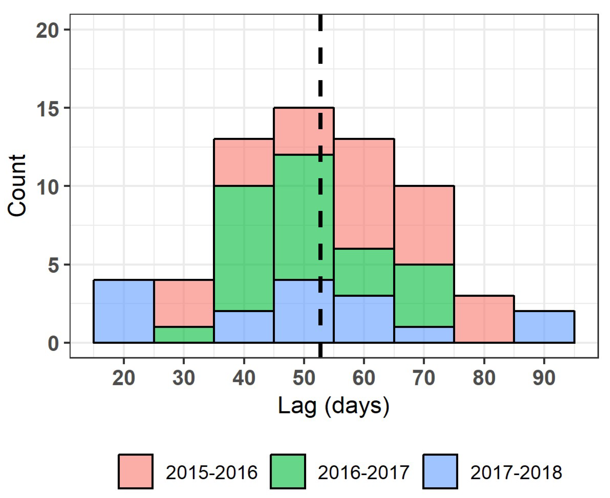
2.4.1. Lag Extraction

The lagged relationship between SMAP SM and LFM needed to be addressed in the following regression model. We compared the two series at every site to extract the time difference between SMAP SM and LFM. In this step, VARI calculated using MODIS MD43A4 daily reflectance was used as a proxy of LFM to obtain a smoother time series and mitigate the problem of missing values, which harms the accuracy derivation of key timing points to describe the annual cycle of change. As a reflectance of vegetation health condition and water content, VARI has little to no temporal lags to the change of LFM and captures the dynamics of LFM well [11]. For SMAP SM and VARI at every site, we derived the key timing of time series including the start, peak, and end of each water year (2015–2016, 2016–2017, 2017–2018). TIMESAT, a MATLAB-based time series analysis package, was used for this step [49]. The start and end of VARI was used to reset the calculation of CGDD at the beginning of the next water year. The peak of VARI was used to divide the growing cycle into green-up and brown-down periods. We treated each LFM site differently when calculating the lags between the SMAP SM and LFM. For every water year in the study, we first calculated the difference between the key timing of the SMAP SM and VARI to obtain the lag. Then, we derived the average lag across the three water years as the lag used for data manipulation at each site.

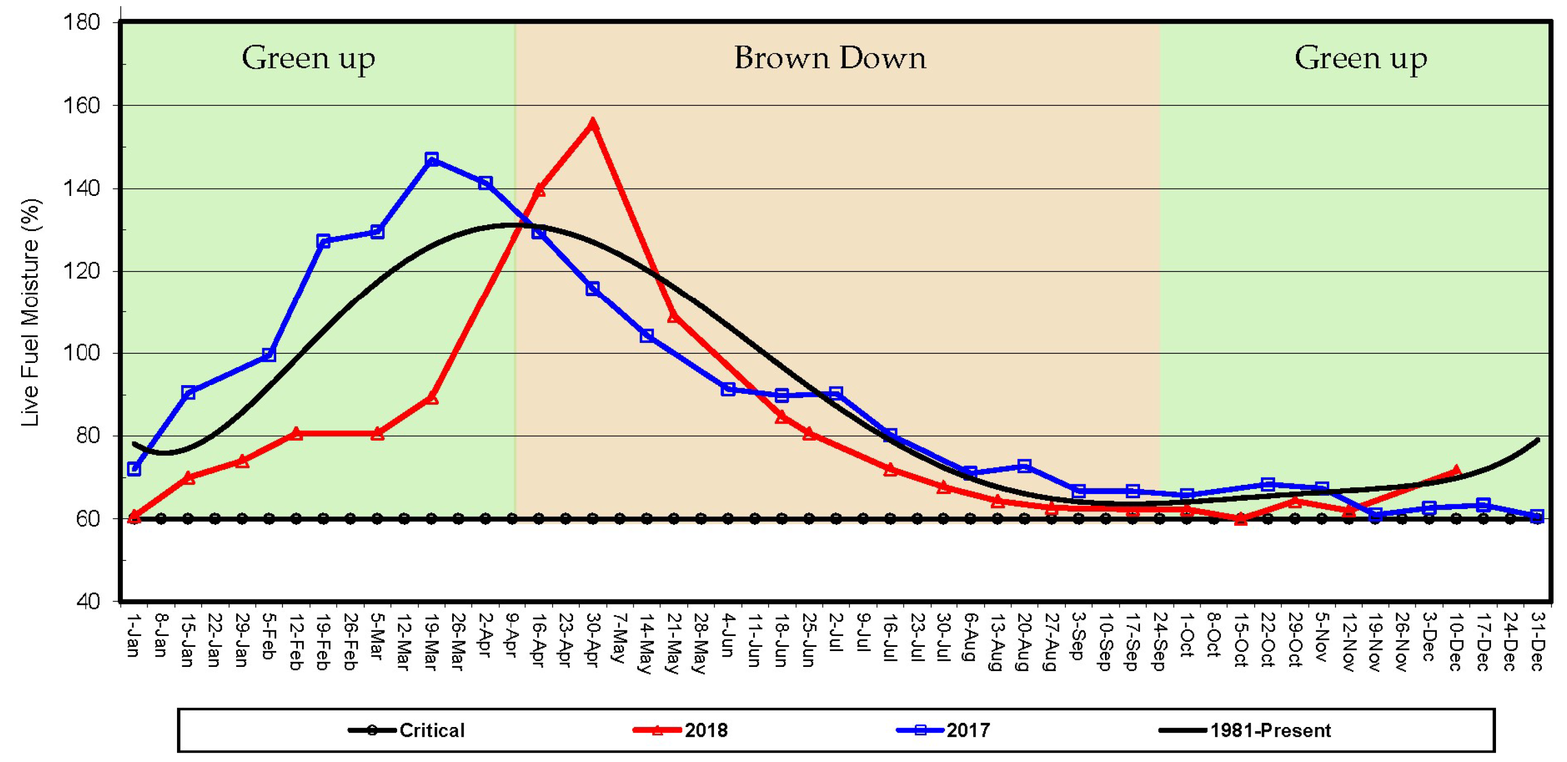
2.4.2. Phenological Phase Definition

We used a new way to address the seasonality of plant growth in this study. Instead of using calendar months to divide seasons in the modeling, we separated the growing cycle using the start, end, and peak time derived using TIMESAT described in Section 2.4.1. The growing cycle of chamise was divided into the green-up and the brown-down periods. Green-up periods start from the time when the first consecutive increase in VARI was identified and end at the peak time of VARI. Brown-down periods start from the peak time of VARI and end when VARI reached the bottom as time proceeds. In the growing cycle of chamise in Southern California, the green-up period is from winter (DJF) to mid-spring (March to mid-April), while the brown-down period runs from mid-spring to summer (JJA), and ends in fall (SON). Using phenological metrics can better account for site-wise and inter-annual differences in the growing cycle than rigid calendar months.

2.4.3. Regression Models Using the Synchronized SMAP SM

We first calculated Kendall’s rank correlation between the LFM and the original SMAP SM. Kendall’s rank correlation was employed as it assesses the strength of relationship between two variables without making any assumptions about the frequency distribution of variables [50]. In addition, Kendall’s rank correlation is less sensitive to the outliers in the data series [51]. We shifted the SMAP SM time series at every LFM site to synchronize with the LFM, using lags between the SMAP SM and LFM at each site obtained by TIMESAT. A new Kendall’s rank correlation was then calculated between LFM and the synchronized SMAP SM for comparison. Later, we built a regression model to estimate LFM using the synchronized SMAP SM and reported adjusted R2 and root mean square error (RMSE) for model performance.
To address the impacts from heat during the growing cycle of chamise, we introduced CGDD as the second independent variable in the regression model. The model was constructed separately for the green-up and brown-down periods to address the different role that CGDD and SMAP SM played before and after plants reached the peak. During the green-up periods, both CGDD and SMAP SM positively contributes to the growth of plants as the determinants of the amount of moisture and heat available to initiate and sustain the growth, which causes an increase of LFM. When plants reach the peak of growth and the vegetation health starts to decline, CGDD has a negative correlation to vegetation health. SMAP SM positively contributes to the LFM as an indicator of surface drought condition, different from the role it played during the green-up period. Separating the two phenological stages can address such difference between the phenological stages for a more physically meaningful model of LFM.

2.4.4. Regression Models Using the Accumulative SMAP SM

Another way to account for the lag between SMAP SM and LFM was using the lag as the size of a leading moving window to calculate the accumulative SMAP SM ahead of the LFM observation. This strategy assumed that the LFM of plants was not determined by a single slice of SMAP SM in the past. Instead, moisture accumulated over a certain period to initiate the growing process and support the plant growth. Once the SM of topsoil increases right after the precipitation, it needs time to be utilized by plants and reflected in the vegetation growth. Furthermore, such contribution also changes over time. The SMAP SM on the day when the LFM measurement is taken may have little to no impact on the LFM observed, as SMAP only measures the SM of topsoil (~5 cm), which needs time to be assimilated by plants. In contrast, moisture stored in the topsoil a few weeks earlier has already infiltrated into the root zone and been assimilated plants, thus plays a greater role than the present moisture in the topsoil in determining the LFM.
In this study, we compared the two strategies to account for the accumulative effect of the SMAP SM on vegetation growth to soil moisture increases. The first was simply adding up all the SMAP SM available in the time window, while the second was applying a weight function to the SMAP SM in the time window then adding them up to address the different contributions to the LFM between the earlier and later SMAP SM measurements. The weight function followed the inversed exponential format, with the weight decreasing from the earliest to the latest date. GDD was also added as the second independent variable to address the contribution from heat. Similar as the model using synchronized SMAP SM and CGDD, the green-up and brown-down periods were calculated separately while building the models. We summarized the equation and physical indication of the four models discussed in Section 2.4.2 and Section 2.4.3 in Table 1.

3. Results

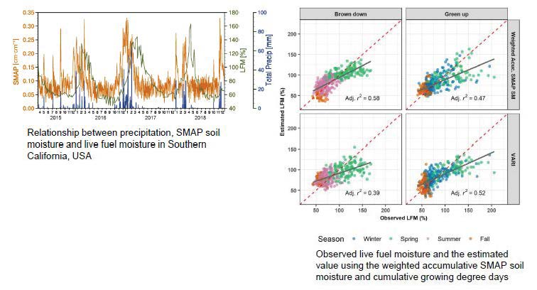
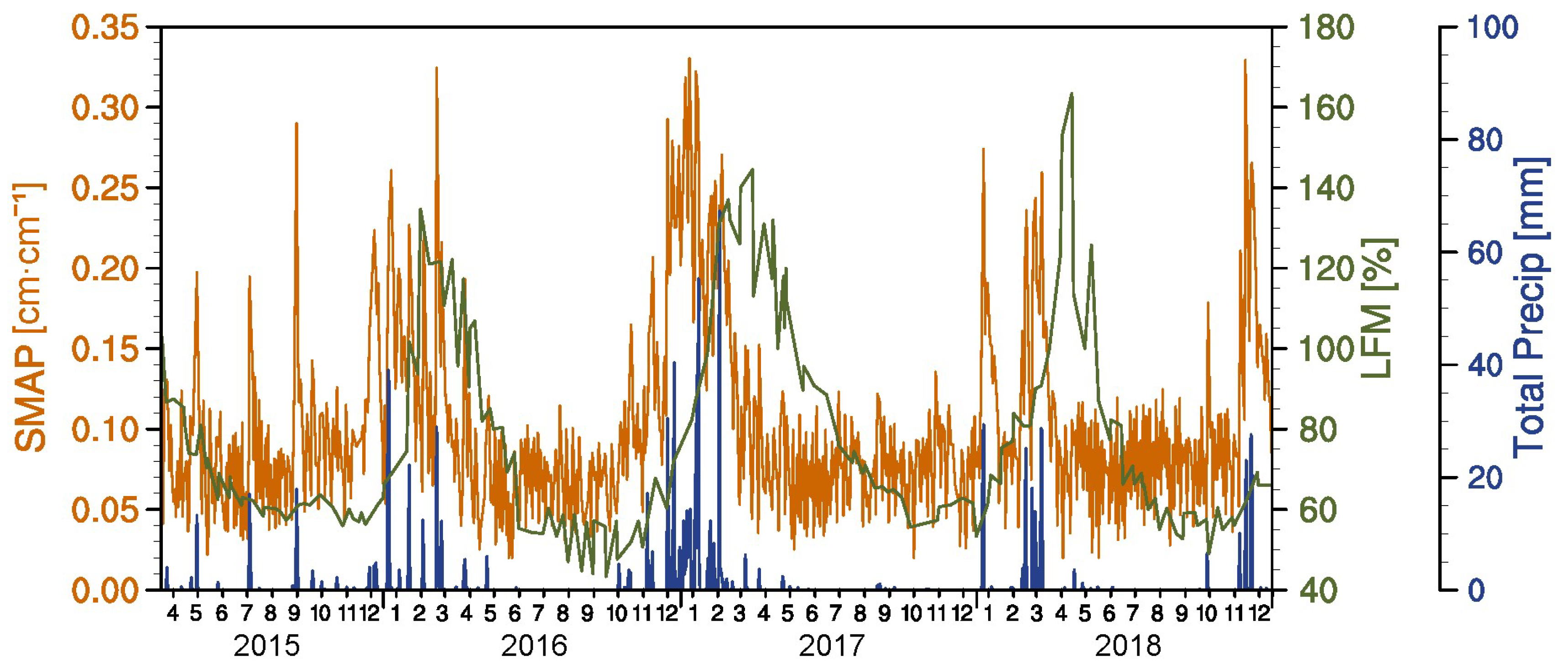
3.1. Relationship between Precipitation, SMAP SM, and LFM

We first compared the average daily precipitation, SMAP SM and LFM across the 12 LFM sites in Southern California to get a better indication of the relationship between the atmospheric moisture supply, moisture in the topsoil, and the growing cycle of chamise. Soil moisture in the topsoil showed an immediate response to the precipitation, while a delay was observed in the response from LFM (Figure 3). This time difference was prominent especially in water year 2016–2017, when the precipitation was concentrated in January and February and formed a significant single peak in the winter months. SMAP SM increased and peaked at the same time as the precipitation occurred, then sharply decreased as the rainy season ended in early March. During the summer and fall months (JJA, SON), the SMAP SM value stayed below 0.15 cm cm−1 without a significant upward or downward incline. On the other hand, LFM reached its peak around April, at the time of maximum blooming, which was several weeks after the peak of SMAP SM and precipitation. LFM started to decrease in mid-April as the temperature continued to grow and reached its minimum in fall (mid-September).
However, there is a significant inter-annual variability between SMAP SM and LFM. Compared with 2016–2017 with a greater amount of precipitation and higher peak LFM of 145%, the total amount of precipitation during the rainy season in water year 2015–2016 was below normal and led to a lower LFM peak value of 130% (Figure 3). The time difference between the peak of SMAP SM and LFM was also short in 2015–2016. The peak of the rainy season did not end until March 6, 2016, the last day when the daily precipitation was above 10 mm. At the same time, the average LFM across the 12 sites was already 120%, indicating that plant growth was near the peak of the growing season. The year 2016–2017 had the strongest rainy season among the three years of study. The accumulative precipitation was 508.7 mm, higher than the 237.5 for 2015–2016 and 225.2 mm for 2017–2018, with a peak of 67 mm on February 18, 2017. Due to a much greater moisture supply, LFM during the growing season was higher than the previous year, with a peak of 144% on March 16, 2017. Compared with the two previous years, the rainy season of 2017–2018 was separated into two sections and started later. The first day with more than 10 mm precipitation was January 1, 2018, much later other years (November 21, 2016 for 2015–2016, November 26, 2016 for 2016–2017). After a dry February without precipitation, a bigger peak of precipitation occurred in late March. The late occurrence of the rainy season also led to a much later time of LFM around April 29, 2018. Though the rainy season was separated into two smaller peaks, the year 2017–2018 had the highest peak LFM (165%) among the three water years of analysis.
The inter-annual variation of precipitation pattern resulted in a large range of the lag between SMAP SM and LFM. In the histogram showing the lags between the SMAP SMs across different years and sites (Figure 4), the majority of lags ranged between 40 and 70 days with an average of 53 days, indicating about a two-month lag between the increase of SMAP SM and the change being reflected in the LFM. Comparing the three water years of study, lags of 2016–2017 had the least outliers and were concentrated around the average. Outliers include two results above 90 days and three below 30 days (Figure 4). Results with the longest lags came from 2017–2018, a water year with two separate peaks in the rainy season. The earlier peak in January did not immediately initiate the growing season for some sites. The separate peaks in the rainy season of 2017–2018 also resulted in three results with less than 30 days of lags (Figure 4), as the second peak of precipitation occurred about less than a month before LFM reached its peak at some sites.

3.2. LFM Estimation Using the Synchronized SMAP SM

We first evaluated the impact of the lag between the SMAP SM and LFM on the relationship between the two variables by calculating the average. Kendall’s rank correlation between the SMAP SM and LFM across all study sites showed that the two variables had a positive but low correlation, with an average Kendall’s τ of 0.19 and a large variation from 0.01 to 0.42 (bottom box in Figure 5). After shifting the SMAP SM time series forward with the length of lag at each site, the correlation was significantly increased to an average of 0.4 (middle box in Figure 5). However, the correlation between the LFM and SMAP SM regardless of the synchronizing of time series or not, was still significantly lower than the LFM and MODIS VARI, which had an average τ of 0.6 (top box in Figure 5).
As the synchronized SMAP SM had a better correlation with LFM, we developed a linear regression model for LFM with the synchronized SMAP SM. The overall adjusted R2 value of this model was 0.358, much lower than 0.442 from the reference model using MODIS VARI (Table 2). The relatively low adjusted R2 can be attributed to the poor performance in 2015–2016 and 2017–2018. In these two years, the estimated LFM had a great discrepancy from the observation. The model significantly overestimated the LFM during the dry seasons (JJA and SON) of both years by 30%, while the model underestimated the LFM in the peak of 2017–2018 by 60% (Figure 6). Overall, the regression model using the synchronized SMAP SM did not yield a satisfactory LFM estimation, especially for 2015–2016 and 2017–2018. This indicated the need for additional independent variables other than SMAP SM to address other factors contributing to vegetation growth and health.

3.3. LFM Estimation with the Consideration of GDD

Many environmental factors are involved at each plant developmental stage other than SM. In this study we employed temperature effects in the form of CGDD in the regression model to estimate LFM. CGDD describes the heat accumulation necessary for plant development and the condition of drought. During the green-up period when plants actively grow, CGDD associated with plant growth positively. When the brown-down period starts, CGDD continues to grow and contributes to vegetation health negatively as an indicator of moisture loss due to evaporation.
We separated the brown-down and green-up periods by the peak day of LFM in the modeling to address the difference between the two different phenological stages. The model with CGDD employed showed a higher overall adjusted R2 and a lower RMSE than models using the synchronized SMAP SM (Table 2). However, such an improvement was much more prominent in the model for the brown-down period. The adjusted R2 was 0.51 for the model using synchronized SMAP SM and CGDD (Figure 7a), significantly higher than the reference model using MODIS VARI (adjusted R2 = 0.38). Compared with the reference model, results from the new model during the brown-down period also contained less outliers. The adjusted R2 of the CGDD only model to estimate LFM was also significantly higher in the brown-down period (Table 2), indicating that the CGDD mostly contributed to the estimation of the LFM when plants experience withering. However, the underestimation of high LFM in the spring was still persistent, especially when plants just passed the peak and still stayed above 150% (red box in Figure 7a).
On the other hand, the new model was outperformed by the VARI-only model in the green-up period due to the underestimation of high LFM values in winter and spring (Figure 7b). The introduction of GDD did not improve the modelling outcome of wet seasons (winter and spring) when the growth of vegetation was active. LFMs above 100% were significantly underestimated in the new model (red box in Figure 7b) compared with the VARI-only model. The adjusted R2 was 0.173 for winter and 0.096 for spring, similar to the single variable model using the synchronized SMAP SM (Table 2).

3.4. LFM Estimation Using the Accumulated SMAP SM

The most prominent weakness in the two previous models was the significant underestimation during the active growing periods and when LFM was high. To better address the supply of moisture in the growing cycle of plants, we replaced the synchronized SMAP SM with an accumulative SMAP SM calculated within a leading time window before the LFM observation.
The use of accumulative SMAP SM alleviated the underestimation of high LFM (>100%) in winter and spring for the green-up period (red box in Figure 7b and Figure 8a). Such improvements also significantly increased the adjusted R2 from 0.27 to 0.43 (Table 2). The brown-down period had a less prominent improvement, with an adjusted R2 from 0.5 to 0.56 (Table 2). These results showed that the use of accumulative SMAP SM better described the impact of soil moisture on the growth of plants. In addition, adopting the accumulative SMAP SM significantly increased the number of LFM observations that could be used for model construction. A large number of the LFM observations were not included in the models using synchronized SMAP SM due to the lack of a paired SMAP SM measurement. Employing the accumulative SMAP SM provided more SMAP SM-related data to pair with the LFM observations, which was crucial for the construction of multi-variant regression models and the production of LFM estimation.
To include various contribution from SM over time, a weight function was applied when the SMAP SM was accumulated. Results showed that adding a weight function in the calculation of accumulative SMAP SM improved the green-up period and the overall adjusted R2 slightly from 0.51 to 0.53 (Table 2). Such improvements occurred only in the green-up period, whose adjusted R2 increased from 0.43 to 0.47 (Table 2 and Figure 8b). By far, the model using weighted accumulative SMAP SM and CGDD yielded the highest overall adjusted R2 and the smallest RMSE among all the models involving SMAP SM as well as the reference model using MODIS VARI (Table 2). Although this model has a lower adjusted R2 than another reference model using MODIS VARI and CGDD (adjusted R2 = 0.56), it still provided the LFM estimation with the lowest RMSE (19.876%) among all models discussed (Table 2).

3.5. Model Comparison and Validation

The outcome from the four models discussed above were compared with the observed LFM for validation. The model using weighted accumulative SMAP SM and CGDD had the highest adjusted R2 among all the models discussed in this study (bold text, Table 2), including the reference model using MODIS VARI. Different model’s performance depended on the level of overestimation or underestimation near the peak of the LFM. Models with CGDD employed as the second variable performed better in the brown-down period as the overestimation was relieved. The discrepancy to the observation around October of 2016 and 2018 was around 10% for the best performing model using the weighted accumulative SMAP SM and CGDD (red line, Figure 9). The adjusted R2 of these models had an average of 0.54 for the brown-down period, much higher than the VARI model (adjusted R2 = 0.37). The factor that harmed the performance of all models discussed in this study was the prominent underestimation of high LFM values, especially those that were obtained near the peak of LFM in spring (Figure 7 and Figure 8). Adopting the accumulative SMAP SM alleviated this issue. This improvement increased the adjusted R2 from 0.25 to 0.43 and 0.47 for the non-weighted and weighted accumulative SMAP SM respectively (Figure 8). However, models could not reproduce the high LFM observations between 150% and 200%, including the reference model using MODIS VARI.
Model performance also differed across years. Among the three years of study, the year 2017–2018 had the greatest discrepancy in the estimation of peak values. The less concentrated precipitation during winter of this year led to a slower climb in the LFM, which was well-captured by models. Models could not reproduce the sharp increase near the peak of the LFM. Yet this discrepancy has less of an impact on the use of the model for fire risk estimation, as the fire risk is at its minimum around the peak of the LFM. Although the estimation of LFM was very close to the observation during the climbing and declining times, models significantly underestimated the LFM near the peak and overestimated near the minimum for the year 2016–2017 (Figure 9). The model using the weighted accumulative SMAP SM and GDD was the one with the smallest discrepancy in the estimation of this year. The year 2015–2016 had a noisier estimation than other years during the green-up period (from December to mid-March), though this year had the smallest discrepancy near the peak.
Overall, the LFM estimation model represented the increasing and decreasing trends of the LFM relatively well. The use of weighted accumulative SMAP SM and CGDD improved model performance in all years of the study. Under and over estimation near the extremes was a persistent problem of all models, although introducing new independent variables slightly relieved such discrepancies.

4. Discussion

4.1. SMAP SM for LFM Estimation and Outlook

Our results showed that the L-band soil moisture can serve as a new metric for LFM estimation, if appropriately processed and combined with other metrics to address the interaction between weather conditions and plant physiological processes. Compared with the vegetation indices obtained from optical remote sensing products, SMAP SM from L-band radiometers are less prone to disturbances from weather conditions, extending its application to some circumstances with unfavorable weather for optical satellite observation. Furthermore, SMAP SM describes the available moisture in the soil that can be utilized to initiate and sustain plant growth, which directly addresses plant physiological processes.
Although the model using weighted accumulative SM and CGDD outperformed the reference model using MODIS VARI and yielded the smallest RMSE, it still had a lower adjusted R2 than another reference model using MODIS VARI and CGDD (Table 2, Figure S3). However, VARI represents the spectral response of plants at different hydric statuses or under different levels of water stress, which is a result of changes in moisture and heat. Therefore, the impact from heat has been included implicitly in the dynamics of VARI, leading to a strong collinearity between the independent variables. In contrast, the accumulative SM and CGDD employed in our best LFM model are two independent metrics addressing contributions from moisture and heat. Compared with the VARI + CGDD model, it described the process of hydrological circulation between the soil and vegetation in a more physically reasonable way.
The use of leading time lag between SMAP SM and LFM was crucial in LFM modeling using SMAP SM. The present study also showed a better estimation of LFM than a similar study for the Mediterranean region using the root zone SM and microwave indices like VOD at X-band and Microwave Polarization Difference Index (MPDI) derived using measurements from ESA’s SMOS program [7]. Part of the improvement in the present study arose from the adoption of accumulative SMAP SM, whose calculation highly depended on the derivation of the lag time between SMAP SM and LFM. Such a lag describes the time needed in the plant’s physiological process to absorb root zone SM and assimilate the nutrients that support growth. Our study addressed this lag by employing accumulative SMAP SM. It can also serve as an approach to calculate the outlook of LFM using remotely sensed SM weeks before, which can be used in fire risk alarming.
Unlike the study focusing on LFM in the Mediterranean region, we did not employ root zone SM products derived using the surface SM (topsoil ~5 mm). The derived root zone soil moisture (SPL4SMAU) changed simultaneously with the surface SM, which did not help to address the lag relationship between surface SM and LFM (Figure 10). The major improvement in the present study arose from the adoption of accumulative SMAP SM and the use of CGDD, as well as the partitioning of LFM observation by the phenological cycle of plants.
Although we addressed part of the physical process in the terrestrial hydrological circulation between precipitation, soil moisture, and vegetation water content to improve the model outcome, this study still simplified a number of important processes in the circulation. Time needed by the plants to assimilate the supply of soil moisture may be longer than the currently used length, which was the lag between the SMAP SM and LFM. Factors other than the amount of topsoil moisture (SMAP SM) and the integral heat (CGDD) may contribute to determine the time needed to assimilate the precipitation residing in the topsoil to trigger and sustain vegetation growth. An inadequate length of time that fully accounts for the preceding soil moisture contributing to the growth of plants may explain the underestimation of the LFM around the peak time indicated in Figure 7, Figure 8 and Figure 9. Future studies should focus on addressing other factors that account for the physiological processes from the increase of soil moisture to the plant growth. Such improvements can lead to a better outlook of LFM by accounting for the leading time that plants need to assimilate the moisture for the growing cycle.
Furthermore, local and plant-specific factors need to be considered if extending the application of the SMAP SM-based model to a broader geographical extent. In this study, we focused on a homogeneous land cover type and one plant species. If applied to a broader region of study, local factors such as land cover type, the stem factor of plants, and soil texture are necessary variables for consideration. In this study, we found there was a difference between the coastal and mountainous sites. Rooted in a more fertile soil type (luvisols) with a significantly smaller proportion of gravel, coastal sites preserve more moisture in the soil, which may explain better performance in the model using accumulative SM and CGDD, especially during the brown-down period (Figure 11). In the brown-down period, the available moisture stored in the soil becomes the vital water supply to sustain the photosynthesis of plants. Coastal sites not only preserve more water input from precipitation in the soil, but are also exposed to a smaller loss of moisture due to the higher humidity from fog/cloud and the moist sea breeze. Such difference across sites needs further investigation if extended to a greater geographical area. Lastly, a combination of LFM observation over different species at each site should be used to address the mixed signals from land surfaces covered by pixels of 9 km × 9 km of SMAP SM.

4.2. Separating Green-up and Brown-down Period for LFM Modeling

All the multi-variant models using SMAP SM and CGDD discussed in this study were constructed separately for the green-up and brown-down periods divided by key phenological metrics, such as peak time, season start, and season end. Compared with dividing data by fixed calendar months to differentiate between seasons, this strategy better addressed seasonality in the LFM time series by accounting for actual phenological processes. As the phenological metrics were calculated by year and by site, they better described the inter-annual and cross-site changes of the growing season than fixed calendar months in previous studies [11].
In addition, modeling LFM separately for the brown-down and green-up periods also accounted for the different roles that SMAP SM and CGDD played in these two different phenological stages of plant growth. During the green-up period, both factors positively contribute to the growth of chamise and determine the amount of biomass accumulated in this period. After chamise becomes mature and reaches its peak growth, the blooming season ends and the biomass starts to wither. During the withering or brown-down period, CGDD continues to grow and impacts vegetation water content negatively, due to the loss of moisture through evaporation [52]. In addition, the green-up of chamise cannot be initiated during the brown-down period even if an abnormal precipitation event occurs. Therefore, the SMAP SM also plays a different role than during the green-up period, even if it maintains a positive correlation with the LFM. During the brown-down period, the SMAP SM describes the present moisture status in the topsoil, an indicator of dryness of the land surface and fire risk. Compared with studies that differentiate between seasons for modeling [11,18], it is more reasonable to build multi-variant models separately for the green-up and brown-down periods and combine the outcomes together to obtain a full time series of estimated LFM.

5. Conclusions

SMAP L-band SM products measure soil moisture residing in the top soil, which serves as a reservoir for a series of physiological processes in the growing cycle of plants. SMAP L-band SM provided a new possibility to construct empirical regression models to estimate LFM, a key observation of vegetation water content for many fire alarm models. Our study on chamise, a wide-spread species of Mediterranean chaparral in Southern California, USA demonstrated that there was a time lead of about 60 days in the change of SMAP SM compared with the LFM of chamise. Compared with shifting the time series to synchronize the SMAP SM to LFM, multi-variant models using the accumulative SMAP SM calculated using a leading moving window at a size of the lag between SMAP SM and LFM performed better. Furthermore, we applied a weight function to address the decaying impact from moisture in the topsoil measured by SMAP SM, which outperformed the model using non-weighted accumulative SMAP SM.
In addition, cumulative GDD (CGDD) as the second variable in the model addressed the heat needed during the growing cycle and the loss of topsoil moisture that influenced the change of LFM. We also found distinguishing the green-up and brown-down periods in the growing season of chamise was helpful to address the different roles that SMAP SM and CGDD played during the growing season. In conclusion, our investigation for Mediterranean chaparral in Southern California indicated that the multi-variant model using a weighted accumulative SMAP SM and the CGDD performed the best in estimating the LFM of chamise. Our model using weighted accumulative SMAP SM and CGDD yielded an adjusted R2 of 0.529 and an RMSE of 19.876, better than the other SM-based model and the reference model using MODIS VARI. This model also provided a possible way to calculate the outlook of LFM using a remotely-sensed land surface metric obtained several weeks ago. Although there was a significant improvement in the estimation of LFM in the brown-down period compared with other models discussed in this study, the underestimation of LFM near its peak was still prominent in our best model.
Future improvements of the study include a more thorough investigation of the determining factors of the physical processes from the increase of moisture in the topsoil to the assimilation of moisture by plants. This will help to better determine the size of the leading moving window in the calculation of accumulative SMAP SM. To reflect the mixed vegetation signal in the 9-km pixel, different species of LFM data are required to be incorporated in the model. The model also needs to be tested on a larger geographical extent and a longer period using other available L-band soil moisture measurement (e.g., SMOS from ESA) or modeled soil moisture products (e.g., ESA Soil Moisture Climate Change Initiative (CCI)). Local factors such as land cover and soil type should be considered when extending the geographical area of study.

Supplementary Materials

The following are available online at https://www.mdpi.com/2072-4292/11/13/1575/s1, Table S1: Soil texture of LFM sites used in the study, Figure S1: Averaged LFM in Southern California and VOD derived from SMAP L-band soil moisture using the multi-temporal dual-channel retrieval algorithm (MT-DCA), Figure S2: Scatterplot of LFM and VOD for LFM sites in Southern California. Colors indicate different seasons, Figure S3: Averaged LFM, Vegetation Opacity (VO), and smoothed VO using 10-day moving average across LFM sites in Southern California, Figure S4: Estimated LFM using VARI + Cumulative GDD. Panels indicate models built for brown down and green up period, as well as the entire dataset Soil texture information is obtained from the Harmonized World Soil Database (version 1.2).

Author Contributions

Conceptualization, S.J. and S.H.K.; Data curation, S.J.; Formal analysis, S.J. and S.H.K.; passive microwave remote sensing and SMAP data characteristics, S.V.N.; Methodology, S.J.; Supervision, M.K.; Visualization, S.J. and S.H.K.; Writing—original draft, S.J.; Writing—review & editing, S.J., S.H.K., S.V.N. and M.K.

Funding

The research at the Jet Propulsion Laboratory, California Institute of Technology, was carried out under a contract with the National Aeronautics and Space Administration (NASA).

Acknowledgments

The research carried out at the Jet Propulsion Laboratory, California Institute of Technology, was supported by the NASA Land-Cover and Land-Use Change (LCLUC) Program. We thank Kristen Whitney from Center of Excellence in Earth Systems Observations (CEESMO), Chapman University for her helps on study conceptualization and reviewing the manuscript. We also thank Alex Konings from Stanford University for providing the vegetation optical depth data derived from SMAP L-band soil moisture products.

Conflicts of Interest

The authors declare no conflict of interest.

References

  1. Syphard, A.D.; Radeloff, V.C.; Keuler, N.S.; Taylor, R.S.; Hawbaker, T.J.; Stewart, S.I.; Clayton, M.K. Predicting spatial patterns of fire on a southern California landscape. Int. J. Wildland Fire 2008, 17, 602–613. [Google Scholar] [CrossRef]
  2. Keeley, J.E.; Syphard, A.D. Climate change and future fire regimes: Examples from California. Geosci. Can. 2016, 6, 37. [Google Scholar] [CrossRef]
  3. Simard, A.J. The Moisture Content of Forest Fuels; University of California: Oakland, CA, USA, 1968. [Google Scholar]
  4. Services, E.G.B.P. National Fuel Moisture Database 2009 User Guide; U.S. Forest Service: Salt Lake City, UT, USA, 2009.
  5. Bradshaw, L.S.; Deeming, J.E.; Burgan, R.E.; Cohen, J.D. The 1978 National Fire-Danger Rating System: Technical Documentation. General Technical Report INT-169; Department of Agriculture, Forest Service, Intermountain Forest and Range Experiment Station: Ogden, UT, USA, 1984; Volume 169, p. 44.
  6. Chuvieco, E.; Cocero, D.; Riano, D.; Martin, P.; Martınez-Vega, J.; de la Riva, J.; Perez, F. Combining NDVI and surface temperature for the estimation of live fuel moisture content in forest fire danger rating. Remote Sens. Environ. 2004, 92, 322–331. [Google Scholar] [CrossRef]
  7. Fan, L.; Wigneron, J.-P.; Xiao, Q.; Al-Yaari, A.; Wen, J.; Martin-StPaul, N.; Dupuy, J.-L.; Pimont, F.; Al Bitar, A.; Fernandez-Moran, R. Evaluation of microwave remote sensing for monitoring live fuel moisture content in the Mediterranean region. Remote Sens. Environ. 2018, 205, 210–223. [Google Scholar] [CrossRef]
  8. Yebra, M.; Chuvieco, E.; Riano, D. Estimation of live fuel moisture content from MODIS images for fire risk assessment. Agric. For. Meteorol. 2008, 148, 523–536. [Google Scholar] [CrossRef]
  9. Yebra, M.; Quan, X.W.; Riano, D.; Larraondo, P.R.; van Dijk, A.I.J.M.; Cary, G.J. A fuel moisture content and flammability monitoring methodology for continental Australia based on optical remote sensing. Remote Sens. Environ. 2018, 212, 260–272. [Google Scholar] [CrossRef]
  10. Jurdao, S.; Yebra, M.; Guerschman, J.P.; Chuvieco, E. Regional estimation of woodland moisture content by inverting Radiative Transfer Models. Remote Sens. Environ. 2013, 132, 59–70. [Google Scholar] [CrossRef]
  11. Peterson, S.H.; Roberts, D.A.; Dennison, P.E. Mapping live fuel moisture with MODIS data: A multiple regression approach. Remote Sens. Environ. 2008, 112, 4272–4284. [Google Scholar] [CrossRef]
  12. Myoung, B.; Kim, S.H.; Nghiem, S.V.; Jia, S.; Whitney, K.; Kafatos, M.C. Estimating Live Fuel Moisture from MODIS Satellite Data for Wildfire Danger Assessment in Southern California USA. Remote Sens. 2018, 10, 87. [Google Scholar] [CrossRef]
  13. Roberts, D.A.; Dennison, P.E.; Peterson, S.; Sweeney, S.; Rechel, J. Evaluation of airborne visible/infrared imaging spectrometer (AVIRIS) and moderate resolution imaging spectrometer (MODIS) measures of live fuel moisture and fuel condition in a shrubland ecosystem in southern California. J. Geophys. Res. Biogeosci. 2006, 111. [Google Scholar] [CrossRef]
  14. Yebra, M.; Dennison, P.E.; Chuvieco, E.; Riano, D.; Zylstra, P.; Hunt, E.R.; Danson, F.M.; Qi, Y.; Jurdao, S. A global review of remote sensing of live fuel moisture content for fire danger assessment: Moving towards operational products. Remote Sens. Environ. 2013, 136, 455–468. [Google Scholar] [CrossRef]
  15. Danson, F.; Bowyer, P. Estimating live fuel moisture content from remotely sensed reflectance. Remote Sens. Environ. 2004, 92, 309–321. [Google Scholar] [CrossRef]
  16. Palmer, K.F.; Williams, D. Optical properties of water in the near infrared. JOSA 1974, 64, 1107–1110. [Google Scholar] [CrossRef]
  17. Qi, Y.; Dennison, P.E.; Spencer, J.; Riaño, D. Monitoring Live Fuel Moisture Using Soil Moisture and Remote Sensing Proxies. Fire Ecol. 2012, 8, 71–87. [Google Scholar] [CrossRef]
  18. Peterson, S.H.; Moritz, M.A.; Morais, M.E.; Dennison, P.E.; Carlson, J.M. Modelling long-term fire regimes of southern California shrublands. Int. J. Wildland Fire 2011, 20, 1–16. [Google Scholar] [CrossRef] [Green Version]
  19. Entekhabi, D.; Yueh, S.; O’Neill, P.E.; Kellogg, K.H.; Allen, A.; Bindlish, R.; Brown, M.; Chan, S.; Colliander, A.; Crow, W.T. SMAP Handbook–Soil Moisture Active Passive: Mapping Soil Moisture and Freeze/Thaw from Space; JPL Publication: Pasadena, CA, USA, 2014. [Google Scholar]
  20. Kerr, Y.H.; Waldteufel, P.; Wigneron, J.-P.; Delwart, S.; Cabot, F.; Boutin, J.; Escorihuela, M.-J.; Font, J.; Reul, N.; Gruhier, C. The SMOS mission: New tool for monitoring key elements ofthe global water cycle. Proc. IEEE 2010, 98, 666–687. [Google Scholar] [CrossRef]
  21. Fournier, S.; Reager, J.; Lee, T.; Vazquez-Cuervo, J.; David, C.; Gierach, M. SMAP observes flooding from land to sea: The Texas event of 2015. Geophys. Res. Lett. 2016, 43, 10338–310346. [Google Scholar] [CrossRef]
  22. Mishra, A.; Vu, T.; Veettil, A.V.; Entekhabi, D. Drought monitoring with soil moisture active passive (SMAP) measurements. J. Hydrol. 2017, 552, 620–632. [Google Scholar] [CrossRef]
  23. Felfelani, F.; Pokhrel, Y.; Guan, K.; Lawrence, D.M. Utilizing SMAP Soil Moisture Data to Constrain Irrigation in the Community Land Model. Geophys. Res. Lett. 2018, 45, 12892–12902. [Google Scholar] [CrossRef]
  24. Jones, L.A.; Kimball, J.S.; Reichle, R.H.; Madani, N.; Glassy, J.; Ardizzone, J.V.; Colliander, A.; Cleverly, J.; Desai, A.R.; Eamus, D. The SMAP Level 4 Carbon Product for Monitoring Ecosystem Land–Atmosphere CO2 Exchange. IEEE Trans. Geosci. Remote Sens. 2017, 55, 6517–6532. [Google Scholar] [CrossRef]
  25. He, L.; Chen, J.M.; Liu, J.; Bélair, S.; Luo, X. Assessment of SMAP soil moisture for global simulation of gross primary production. J. Geophys. Res. Biogeosci. 2017, 122, 1549–1563. [Google Scholar] [CrossRef]
  26. Keeley, J.E. Fire intensity, fire severity and burn severity: A brief review and suggested usage. Int. J. Wildland Fire 2009, 18, 116–126. [Google Scholar] [CrossRef]
  27. Konings, A.G.; Piles, M.; Rötzer, K.; McColl, K.A.; Chan, S.K.; Entekhabi, D. Vegetation optical depth and scattering albedo retrieval using time series of dual-polarized L-band radiometer observations. Remote Sens. Environ. 2016, 172, 178–189. [Google Scholar] [CrossRef]
  28. Chaparro, D.; Piles, M.; Vall-llossera, M.; Camps, A.; Konings, A.G.; Entekhabi, D. L-band vegetation optical depth seasonal metrics for crop yield assessment. Remote Sens. Environ. 2018, 212, 249–259. [Google Scholar] [CrossRef]
  29. Chaparro, D.; Vall-llossera, M.; Piles, M.; Camps, A.; Rüdiger, C.; Riera-Tatché, R. Predicting the Extent of Wildfires Using Remotely Sensed Soil Moisture and Temperature Trends. IEEE J. Sel. Top. Appl. Earth Obs. Remote Sens. 2016, 9, 2818–2829. [Google Scholar] [CrossRef] [Green Version]
  30. Holgate, C.M.; van Dijk, A.I.J.M.; Cary, G.J.; Yebra, M. Using alternative soil moisture estimates in the McArthur Forest Fire Danger Index. Int. J. Wildland Fire 2017, 26, 806–819. [Google Scholar] [CrossRef]
  31. Barbour, M.G.; Keeler-Wolf, T.; Schoenherr, A.A. Terrestrial Vegetation of California; University of California Press: Berkeley, CA, USA, 2007. [Google Scholar]
  32. Weise, D.R.; Hartford, R.A.; Mahaffey, L. Assessing Live Fuel Moisture for Fire Management Applications; United States Department of Agriculture: Washington, DC, USA, 1998; pp. 49–55.
  33. National Plant Data Team, The PLANTS Database. Available online: https://plants.sc.egov.usda.gov/ (accessed on 18 May 2019).
  34. Jow, W.M.; Bullock, S.H.; Kummerow, J. Leaf turnover rates of Adenostoma fasciculatum (Rosaceae). Am. J. Bot. 1980, 67, 256–261. [Google Scholar] [CrossRef]
  35. Wohlgemuth, P.M.; Lilley, K.A. Sediment Delivery, Flood Control, and Physical Ecosystem Services in Southern California Chaparral Landscapes. In Valuing Chaparral: Ecological, Socio-Economic, and Management Perspectives; Underwood, E.C., Safford, H.D., Molinari, N.A., Keeley, J.E., Eds.; Springer International Publishing: Berlin, Germany, 2018; pp. 181–205. [Google Scholar]
  36. Sean, A.P.; Carol, M.; John, T.A.; Lisa, M.H.; Marc-Andr, P.; Solomon, Z.D. How will climate change affect wildland fire severity in the western US? Environ. Res. Lett. 2016, 11, 035002. [Google Scholar] [Green Version]
  37. U.S. Forest Service, National Fuel Moisture Database. Available online: https://www.wfas.net/index.php/national-fuel-moisture-database-moisture-drought-103 (accessed on 1 February 2019).
  38. FAO/IIASA/ISRIC/ISSCAS/JRC. Harmonized World Soil Database (Version 1.2), 2012th ed.; FAO: Rome, Italy; IIASA: Laxenburg, Austria, 2012. [Google Scholar]
  39. Kim, S.-b.; van Zyl, J.; Dunbar, S.; Njoku, E.; Johnson, J.; Moghaddam, M.; Shi, J.; Tsang, L. SMAP L2 & L3 Radar Soil Moisture (Active) Data Products; Jet Propulsion Laboratory: Pasadena, CA, USA, 2012.
  40. O’Neill, P.E.; Chan, S.; Njoku, G.E.; Jackson, T.; Bindlish, R. SMAP Enhanced L3 Radiometer Global Daily 9 Km EASE-Grid Soil Moisture, Version 2; NASA National Snow and Ice Data Center Distributed Active Archive Center: Boulder, CO, USA, 2018.
  41. Chan, S.K.; Bindlish, R.; O’Neill, P.; Jackson, T.; Njoku, E.; Dunbar, S.; Chaubell, J.; Piepmeier, J.; Yueh, S.; Entekhabi, D.; et al. Development and assessment of the SMAP enhanced passive soil moisture product. Remote Sens. Environ. 2018, 204, 931–941. [Google Scholar] [CrossRef]
  42. Ford, T.W.; Quiring, S.M. Comparison of Contemporary In Situ, Model, and Satellite Remote Sensing Soil Moisture With a Focus on Drought Monitoring. Water Resour. Res. 2019, 55, 1565–1582. [Google Scholar] [CrossRef]
  43. Steven Chan, R.B.; Hunt, R.; Jackson, T.; Kimball, J. Soil Moisture Active Passive (SMAP) Ancillary Data Report: Vegetation Water Content; Jet Propulsion Laboratory: Pasadena, CA, USA; California Instite of Technology: Pasadena, CA, USA, 2013.
  44. Prentice, I.C.; Cramer, W.; Harrison, S.P.; Leemans, R.; Monserud, R.A.; Solomon, A.M. Special Paper: A Global Biome Model Based on Plant Physiology and Dominance, Soil Properties and Climate. J. Biogeogr. 1992, 19, 117–134. [Google Scholar] [CrossRef]
  45. Bollero, G.A.; Bullock, D.G.; Hollinger, S.E. Soil Temperature and Planting Date Effects on Corn Yield, Leaf Area, and Plant Development. Agron. J. 1996, 88, 385–390. [Google Scholar] [CrossRef]
  46. Crimmins, T.M.; Marsh, R.L.; Switzer, J.R.; Crimmins, M.A.; Gerst, K.L.; Rosemartin, A.H.; Weltzin, J.F. USA National Phenology Network Gridded Products Documentation; US Geological Survey: Reston, VA, USA, 2017.
  47. PRISM Climate Group. PRISM Gridded Climate Data. Available online: http://prism.oregonstate.edu/ (accessed on 4 February 2019).
  48. Di Luzio, M.; Johnson, G.L.; Daly, C.; Eischeid, J.K.; Arnold, J.G. Constructing retrospective gridded daily precipitation and temperature datasets for the conterminous United States. J. Appl. Meteorol. Clim. 2008, 47, 475–497. [Google Scholar] [CrossRef]
  49. Eklundh, L.; Jönsson, P. TIMESAT: A Software Package for Time-Series Processing and Assessment of Vegetation Dynamics. In Remote Sensing Time Series; Kuenzer, C., Dech, S., Wagner, W., Eds.; Springer: Berlin, Germany, 2015; pp. 141–158. [Google Scholar]
  50. Hauke, J.; Kossowski, T. Comparison of values of Pearson’s and Spearman’s correlation coefficients on the same sets of data. Quaest. Geogr. 2011, 30, 87–93. [Google Scholar] [CrossRef]
  51. Noether, G.E. Why Kendall Tau? Teach. Stat. 1981, 3, 41–43. [Google Scholar] [CrossRef]
  52. Ruffault, J.; Martin-St Paul, N.; Pimont, F.; Dupuy, J.L. How well do meteorological drought indices predict live fuel moisture content (LFMC)? An assessment for wildfire research and operations in Mediterranean ecosystems. Agric. For. Meteorol. 2018, 262, 391–401. [Google Scholar] [CrossRef]
Figure 1. Multi-year average live fuel moisture (LFM) and its dynamics of 2017 (blue) and 2018 (red) in Los Angeles Basin, Southern California (source: County of Los Angeles Fire Prevention Program). The calendar year was divided into green-up (green background) and brown-down (orange background) sections by the direction of the LFM trend across the multi-year average.
Remotesensing 11 01575 g001
Figure 2. Active live fuel moisture (LFM) observation sites and chamise landscape in Southern California. Blue and green dots in the map are sites used in the study, representing coastal and mountainous sites. Grey dots in the map are other sites with data available. Photo shows the landscape of the chamise at the Laurel Canyon site, maintained by Los Angeles County Fire Department.
Remotesensing 11 01575 g002
Figure 3. Averaged SMAP soil moisture (SM) from AM overpasses, chamise LFM observation, and the Parameter-elevation Relationships on Independent Slopes Model (PRISM) daily precipitation across 12 sites of Southern California used in the study. Orange lines are the averaged SMAP SM. Green lines are the averaged LFM observations. Blue bars are the daily precipitation derived from PRISM climate dataset.
Remotesensing 11 01575 g003
Figure 4. Histogram of lags between SMAP SM and LFM of three water years (2015–2016, 2016–2017, 2017–2018) across 12 sites used in the study. Mean length of lag was marked using the dashed line.
Remotesensing 11 01575 g004
Figure 5. Kendall’s tau between LFM and MODIS VARI, SMAP SM, and SMAP SM synchronized to the LFM time series. The average tau across the 12 sites are marked as a diamond in the boxplot.
Remotesensing 11 01575 g005
Figure 6. Multi-site average of the observed LFM (black dots) and estimated LFM (yellow line) using synchronized (sync.) SMAP as the single independent variable across three water years from 2015 to 2018.
Remotesensing 11 01575 g006
Figure 7. Observed LFM and estimated LFM using the synchronized SMAP SM and cumulative GDD (a,b). The brown-down and green-up periods were modeled separately. Outcomes from the VARI-only model were used for comparison (c,d). Data were colored by seasons, using blue for winter, green for spring, pink for summer, and orange for fall.
Remotesensing 11 01575 g007
Figure 8. Observed LFM and estimated LFM using accumulative SMAP SM and CGDD (a) and weighted accumulative SMAP SM and CGDD (b). The brown-down and green-up periods were modeled separately. Outcomes from the VARI-only model were used for comparison. Coloring of data follows the same color code as Figure 7.
Remotesensing 11 01575 g008
Figure 9. Multi-site average of the observed LFM (black dots) and estimated LFM using MODIS VARI (green solid line), and synchronized (sync.) The SMAP SM (yellow solid line) and weighted accumulated SMAP SM with CGDD (red solid line).
Remotesensing 11 01575 g009
Figure 10. SMAP level 3 soil moisture measurements of AM passes (black dots), SMAP level 4 surface soil moisture derivation (blue solid line), and SMAP level 4 root zone soil moisture derivation (red solid line).
Remotesensing 11 01575 g010
Figure 11. Adjusted R2 from single site model for LFM estimation using accumulative SM and CGDD. All models have a p-value < 0.05. The average adjusted R2 across the 12 sites are marked as a diamond in the boxplot. Coastal and mountainous sites are plotted in different panels.
Remotesensing 11 01575 g011
Table 1. Multi-variant regression models discussed in this study and the physical indication. Start of season (SOS) is defined as the first day when a consecutive increase of Visible Atmospheric Resistance Index (VARI) occurs.
ModelEquationExplanation of Model
Synchronized SMAP SM L F M t = α 1 × S M A P   S M t l a g + ε LFM at time t was determinated by SMAP SM at time t-lag
Synchronized SMAP SM + Cumulative GDD L F M t = α 1 × S M A P   S M t l a g + α 2 × S O S t G D D + ε LFM at t was determinated by SMAP SM at time t-lag and the cumulative GDD from the start of water year to t
Accumulative SMAP SM + Cumulative GDD L F M t = α 1 × t l a g t S M A P   S M + α 2 × S O S t G D D + ε LFM at t was determinated by accumulated SMAP SM from t0-lag to t and the cumulative GDD from the start of water year to t
Weighted Accumulative SMAP SM + Cumulative GDD L F M t = α 1 × W × t l a g t S M A P   S M + α 2 × S O S t G D D + ε LFM at t was determinated by the weighted accumulated SMAP SM from t-lag to t and the cumulative GDD from the start of water year to t; weight (W) decreased from past to present in a logarithm form.
VARI only (Reference) L F M t = α 1 × V A R I t + ε LFM at t was determined by VARI at t
Cumulative GDD only L F M t = α 1 × S O S t G D D + ε LFM at t was determined by the cumulative GDD at t
VARI + Cumulative GDD L F M t = α 1 × V A R I t + α 2 × S O S t G D D + ε LFM at t was determined by VARI and cumulative GDD at t
SMAP SM: SMAP soil moisture; GDD: Growing Degree Days.
Table 2. Overall, seasonal, and by section model performance of all models discussed. Model with the highest adjusted R2 using SMAP SM is highlighted in bold text. All models are statistically significant (p-value < 0.001).
ModelAdjusted R2Overall RMSE (%)
OverallBrown downGreen upWinterSpringSummerFall
Synchronized SMAP SM0.358N/AN/A0.1870.0550.2110.01823.202
Synchronized SMAP SM + Cumulative GDD0.4840.510.250.1730.0960.2570.00320.805
Accu. SMAP SM + Cumulative GDD0.5100.560.430.2440.110.2580.00520.284
Weighted Accu. SMAP SM + Cumulative GDD0.5290.580.470.2900.1790.2260.00519.876
VARI only (reference model)0.4420.390.520.3710.1810.0940.00421.628
Cumulative GDD only0.3390.530.150.0170.0120.1380.01023.546
VARI + Cumulative GDD (reference model)0.560.570.5260.3680.1960.1520.00621.467

