Article

Urban Forest Growth and Gap Dynamics Detected by Yearly Repeated Airborne Light Detection and Ranging (LiDAR): A Case Study of Cheonan, South Korea

1
Interdisciplinary Program in Landscape Architecture, Seoul National University, Seoul 08826, Korea
2
Department of Landscape Architecture, Graduate School of Environmental Studies, Seoul National University, Seoul 08826, Korea
3
Department of Contents, Samah Aerial Survey CO., Goyang 10442, Korea
*
Author to whom correspondence should be addressed.
Remote Sens. 2019, 11(13), 1551; https://doi.org/10.3390/rs11131551
Submission received: 29 April 2019 / Revised: 22 June 2019 / Accepted: 27 June 2019 / Published: 29 June 2019
(This article belongs to the Special Issue Remote Sensing of Urban Forests)

Abstract

:
Understanding forest dynamics is important for assessing the health of urban forests, which experience various disturbances, both natural (e.g., treefall events) and artificial (e.g., making space for agricultural fields). Therefore, quantifying three-dimensional changes in canopies is a helpful way to manage and understand urban forests better. Multitemporal airborne light detection and ranging (LiDAR) datasets enable us to quantify the vertical and lateral growth of trees across a landscape scale. The goal of this study is to assess the annual changes in the 3-D structures of canopies and forest gaps in an urban forest using annual airborne LiDAR datasets for 2012–2015. The canopies were classified as high canopies and low canopies by a 5 m height threshold. Then, we generated pixel- and plot-level canopy height models and conducted change detection annually. The vertical growth rates and leaf area index showed consistent values year by year in both canopies, while the spatial distributions of the canopy and leaf area profile (e.g., leaf area density) showed inconsistent changes each year in both canopies. In total, high canopies expanded their foliage from 12 m height, while forest gap edge canopies (including low canopies) expanded their canopies from 5 m height. Annual change detection with LiDAR datasets might inform about both steady growth rates and different characteristics in the changes of vertical canopy structures for both high and low canopies in urban forests.

Graphical Abstract

1. Introduction

Quantifying forest gaps is essential for monitoring the stability of the forest structure because these disturbances can change the light environment and drive forest dynamics [1,2,3,4]. Physical disturbances in forest canopies usually result from deforestation (e.g., making space for agricultural fields) and tree-fall events [1]. Forest gaps could be characterized by their size distribution. The frequency of forest gap areas in natural forests follows a power law distribution. Usually, small openings (formed by wind damage or tree mortality) in natural forests dominate areas in size distribution and show larger scaling exponents, while frequent large openings show smaller scaling exponents. Therefore, by comparing the scaling exponents with other forests, it is possible to compare the degrees of disturbances [2,3].
Urban forests are usually fragile to disturbances because the dense human population leads to severe conditions that can damage the forest directly (e.g., land-cover changes from forested to urbanized areas) [5]. Forest damage such as deforestation and landcover changes could result in relatively larger openings than small openings in forests, and human activities therein may hinder the forest equilibrium or change the forest ecosystems [6]. Particularly in South Korea, small and large mountainous urban forests are very common as they remain green areas after development, and many people use them for leisure activities, agriculture, and private graveyards that are accompanied with canopy openings [7,8,9,10,11,12]. Although many policies try to conserve these urban forests in South Korea, land use in urban forests is complex and can easily undergo harsh disturbances [12,13,14]. Therefore, it is important to monitor forest gaps in urban forests where various natural or anthropogenic disturbances can occur.
Forest surveys are conducted in many countries via onsite sampling of plots that are considered representative of the whole study site. In addition, airborne photogrammetry and satellite imagery are applied to measure the diameter at breast height, stand height, basal area, and species composition using terrestrial field sampling data. However, these traditional methods have certain limitations related to the subjective interpretation of measurement results, low measurement accuracy, and lack of information about vertical canopy structures [15,16,17,18,19,20,21]. To compensate for the limitations of existing research methods, there is a need to improve techniques that can support the assessment of forest growth and biodiversity such as airborne light detection and ranging (LiDAR) [16].
Many studies have suggested that airborne laser scanning (ALS) can be applied to describe vertical forest structures, and the accuracy of stand height estimations has been assessed [19,21]. Although ALS-based tree height estimations are less accurate than those using rigorous field measurements [22], the accuracy is acceptable, and the more efficient coverage of large areas by ALS offsets this weakness [17]. Especially, Vepakomma et al. [6] reported the difference between the effects of natural and anthropogenic linear openings (i.e., steam and roads) with LiDAR data. These days, with its acceptable accuracy and advantages in sensing vertical canopy structures, multitemporal LiDAR surveys have also shown great potential for detecting changes in forest structure [23]. For example, the use of adequate multitemporal airborne LiDAR datasets represents a reliable and efficient method for detecting canopy changes and estimating canopy growth and forest biomass dynamics at a fine temporal resolution [24,25,26,27,28,29,30,31,32,33,34]. Recently, Song et al. [24], Zhao et al. [29], Dalponte et al. [30], and Cao et al. [31] successfully estimated forest biomass dynamics and tree growth in forests using repeated airborne LiDAR data. Moreover, Dalagnol et al. [32] and Rangel et al. [33] reported quantification of canopy dynamics focusing on human-induced disturbances (e.g., logging) by using multitemporal airborne LiDAR data in Amazon forests. Rangel et al. [33] reported that setting a height differences threshold was an efficient way to map logged trees and small gaps usually closed within short periods (within two years). Dalagnol et al. [32] found that gap formation occurred more frequently in logged areas than in intact forests.
For applications of multitemporal ALS in urban forests, a few studies about the forest dynamics (e.g., forest growth and forest gap dynamics) in an urban forest have been conducted. Ossola and Hopton [35] measured urban tree loss dynamics in city residential landscapes using bitemporal (five-year period) LiDAR datasets. They particularly noted the changes in urban trees over time caused by human management and urban tree removal for hazard prevention or artistic preference. Since urban forests are characteristically vulnerable to various and frequent disturbances, particularly in terms of physical damage [4,35,36,37,38,39], canopy loss occurs frequently and could finally result in artificial canopy openings. However, to the best of our knowledge, most studies with airborne LiDAR datasets have focused on forest gaps that are usually treefall gaps in natural forests [26,27,28], and few studies are related to artificial canopy openings in cities. In the same manner of the effect on the surrounding environment of forest gaps, artificial openings could affect the adjacent environment [32,40] and may also affect the changes in surrounding canopy structures. Therefore, it is important to monitor urban forests continuously [41,42] including both forest gaps and their artificial canopy openings.
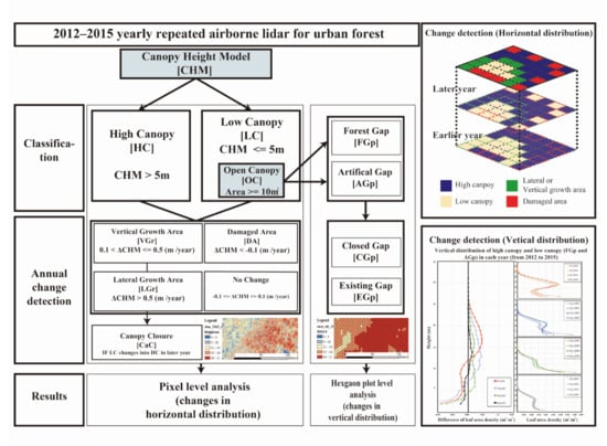
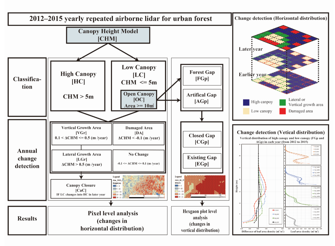
Thus, we estimated three-dimensional canopy changes in an urban forest using four years of annual LiDAR datasets. To assess how much urban forest structures have changed, we estimated: (1) the distribution of the growth area and damaged areas (e.g., vertical and lateral growth as well as damaged areas), (2) changes in the vertical leaf area density profile, and (3) the dynamics of opening and closing forest canopies during 2012–2015. Accordingly, this study addressed two questions: (1) What are the differences between canopy structure changes derived from annual change detections and three-year interval change detection? (2) What are the characteristics of structural changes by different canopy classes (e.g., high canopies and lower canopies) in urban forests?

2. Materials and Methods

2.1. Study Site

The study was conducted at Mt. Bongseo (36.82°N, 127.12°E, altitude: 158 m, area: 124 ha), a remnant patch after urban development located in the center of metropolitan Cheonan, Chungcheongnam-Do, Republic of Korea. The study site is covered with a mixed forest dominated by Quercus acutissima (percent area: 44.8%), Pinus rigida (29.7%), and Larix leptolepis (7.4%). The average age class (as designated by the Korea Forest Service, 2015, http://www.forest.go.kr/) of the forest is 3.8 (i.e., 30–40 years old; the third class). Both managed and unmanaged forest areas can be found within the study site. The forest is easily accessed by citizens, and local amenities such as health facilities are present within the forest. Moreover, some of the land in the site is used as a cemetery and some have agricultural activity, which is private land (Figure 1).

2.2. Field Survey

To classify open canopy types (e.g., natural treefall or thinning, private graveyards, facilities, and agricultural activities), we conducted field trips on 7 October 2016, 26 August 2017, and 26 September 2017. Moreover, to determine how much canopy should be classified as open canopy, we conducted simultaneous localizing and mapping (SLAM) mobile LiDAR (Stencil, Kaarta, PA, USA) scanning under the tree-fall area (Figure 2) at the site on 26 March 2018, when the trees were defoliated. We generated 0.25 × 0.25 m2 digital surface models using the maximum height (HMAX) of all mobile LiDAR datasets with CloudCompare software (https://www.danielgm.net/cc/) and generated canopy height models (CHMs) by subtracting the digital terrain models from the digital surface models. Finally, we calculated the gap size in ArcGIS ver. 10.2.2 (ESRI, Redlands, CA, USA). The average area of the 19 open canopies in the nine sampled plots was calculated as 12.48 ± 9.76 m2 with consideration of the foliated season and previous research by Yamamoto [43] and Runkle [44], who did not consider very small openings (<5 m2) as gaps. For the convenience of calculation, we classified gaps as locations where the open area was 10 m2 or more (Figure 3).

2.3. Airborne Light Detection and Ranging (LiDAR) Dataset Acquisition and Registration

The airborne LiDAR datasets were acquired on 9 October 2012 (day of the year (DOY): 283), 16 May 2013 (DOY: 136), 16 June 2014 (DOY: 167), and 30 October 2015 (DOY: 303) from IGI LiteMapper 6800 (Samah Aerial Survey), which were all during the foliated season. LiDAR data were acquired in different months. However, Song and Ryu [42] reported relatively stable seasonal leaf area index (LAI) values in a forest (in the same climate zone as our study site) in South Korea. Our study site experienced the maximum number of leaves that turned red in the first and last study year on 28 October 2012 and 26 October 2015, respectively (Korea Meteorological Administration, www.kma.go.kr). Therefore, we assumed that our data were acquired in the full-leaved seasons.
The study site was surveyed following eight trajectories (Figure 1) by overlapping 50% of the trajectory edges at an altitude of 1000 m. The beam divergence was 0.3 mrad, and field of view was 60°. All annual point densities were higher than 8 points/m2, which were sufficiently dense and similar in order to effectively compare datasets. The airborne LiDAR datasets were preprocessed using algorithms built into the TerraScan (Terrasolid, Helsinki, Finland) software on the MicroStation (Bentley) platform. First, we filtered noise at low points and aerial points. Second, we used classification algorithms to classify the points into ground and nonground classes. We minimized measurement errors by selecting 190 planar areas over the entire year in the digital surface model generated from the point cloud datasets for 2012, 2013, 2014, and 2015 and matched the heights with the average elevation for 2012. Finally, the height was adjusted based on the ground control points (triangulation point: 36°49′02.09″, 127°07′27.31″, ellipsoidal height: 182.17 m; unified control point: 36°48′50.29″, 127°06′55.92″, ellipsoidal height: 906,045 m; National Geographic Information Institute) and points on the roof of a building detected for all years. We selected 70 new random 16 m2 plots, including building rooftops and roads where the heights were consistently adjacent to the site, to compare the 2012–2014 airborne LiDAR datasets with the 2015 airborne LiDAR dataset. The average differences from the 2015 dataset were –0.01 (2012), –0.04 (2013), and –0.05 m (2014). Although the validation results showed that the heights in 2015 were slightly greater than those in the other years, we concluded that accuracy anomalies in the dataset within 0.1 m were acceptable.

2.4. Generation of Height Models and Change Detection

Since the research site is mountainous, and sloped areas may distort the vertical and horizontal locations of the tree canopy and apex [45,46], we did not consider segmenting the tree apices. Therefore, we simply calculated the vertical differences in CHMs for 2012–2015 that were generated from the LiDAR datasets and estimated the changes in the canopy throughout the study period. Since quantifying the changes of canopy opening areas and identifying the growth direction (i.e., vertical or lateral direction) both require high-resolution CHMs (e.g., [24,27,28]), and the beam divergence of the LiDAR sensor was 0.3 mrad, which is a 0.3 m footprint at the ground level (flight altitude: 1000 m), we assumed that 0.25 × 0.25 m2 grid resolution would be adequate. After preprocessing the LiDAR datasets into 0.25 × 0.25 m2 (grid level survey) digital surface models and digital terrain models, CHMs were generated using the TerraScan software (Figure 4a). The annual average canopy heights for 2012–2015 were 11.09, 11.02, 12.29, and 12.12 m, respectively. The CHMs for each year were classified into two classes: high canopy (HC), with canopy height >5 m, and low canopy (LC), with canopy height ≤5 m (Figure 3). In addition, we included the canopy closure (CaC) subclass, which represents areas with LCs in earlier years that became HCs in later years. Based on the estimated growth rates outlined by Song et al. [24], we assumed that the average annual growth rate of mature trees could not exceed 50 cm/year. Therefore, after calculating the changes between the two years, we classified the growth regions into four subclasses: vertical growth (VGr) areas with annual mean growth rate ≤50 cm, lateral growth (LGr) areas with annual mean growth rate >50 cm; damaged areas with negative growth rates, and no-change areas with –10 to 10 cm growth rates.
Since grid size can affect the accuracy of HMAX estimates [47], and canopy metrics based on vertical profiles can be used to accurately estimate forest structure [34,48], we generated a larger size of grids for the plot level survey using hexagonal grids with an area of 16.24 m2 and edge length of 2.5 m (approximately the mean size of a closed gap area during the study periods) to estimate the changes in vertical profiles, leaf area density (LAD), and canopy complexity.

2.5. Gap Detection and Classification

We set the thresholds of height and area for detecting open canopies as 5 m (which was almost half of the CHMs) and 10 m2 (based on the gap area calculation from mobile LiDAR datasets and for convenience of calculation), respectively, and identified the open canopies (OCs) in each CHM. We defined gaps with canopy openings caused by fallen or dead trees as forest gaps (FGp) and those caused by civic usage as farmland, cemeteries, or trails as artificial gaps (AGp) (Figure 1).
To investigate the size distributions of FGp and AGp, we estimated the scaling exponent (λ) that describes the extent to which disturbances are clustered (i.e., lower λ means frequent large disturbances, while higher λ means frequent small disturbances) [49,50,51] using methods from Asner et al. [51].

2.6. Estimating Changes of Vertical Canopy Distribution and Canopy Complexity

The leaf area index (LAI, m2/m2) and canopy complexity (Rumple index, m2/m2) are well known to correlate with the productivity of forest ecosystems [52,53,54,55]. LAI is usually calculated as half the total leaf area per unit surface area [56,57]. We estimated the LAI and leaf area density (LAD, m2/m3) using the “lidR” package in R software [58] according to the method of Bouvier et al. [52], who calculated the LAI based on the Beer–Lambert theory. The LAD was estimated by dividing the LAI values by dz (the profile of LAD). The canopy complexity was also estimated using the Rumple index function within the “lidR” package. Canopy complexity was calculated as a three-dimensional surface area divided by a two-dimensional surface area, which denotes the structural diversity of canopies [53,54,55,59]. Section 2.6 is summarized in Table 1 and Figure 4.

3. Results

3.1. Pixel and Hexagon Height Model-Based Change Detection

With change detection, we found that changes in the distribution of canopies were irregular year by year (Figure 5), while the annual VGr rates remained relatively stable throughout the study period. There were no great growth rate differences according to either the time interval or the grid size (Table 2). Figure 5a presents an example of the overall distributions of growth and damaged areas in 2012–2015. Figure 5b,c show the vertical changes over two years (i.e., one-year term) to explain the growth and damaged area distributions. Detected growth areas where the canopy height increased usually resulted from lateral growth rather than vertical growth in HCs, which could mean that taller canopy overlapping occurred frequently. In the case of low canopies, lateral growth areas were pervasive in annual change detection, while vertical growth areas were sustained over total periods. Because LC areas included bare lands, the height remained relatively unchanged.
Furthermore, canopy closure (LC to HC) tended to be driven by LGr rather than VGr, possibly because the rate of LGr among taller trees was higher than that of VGr among young trees at the study site (Figure 5d). Besides, we found that disturbance and canopy loss were widespread over the whole study period (Figure 5b,c).

3.2. Continuous One-Year Vertical Growth Area

Due to widespread canopy loss and the complexity of the dynamics in both canopies (Figure 5), we tried to detect continuous growth areas. Table 3 shows the proportion of the area in which the canopy continuously grew upward at pixel (via CHMs) and plot (via hexagonal grids) levels. The proportion of overlapping growth areas with positive values (i.e., gradual vertical canopy growth) based on the height difference for 2012–2015 showed a 15.9% correspondence at the pixel scale and a 38.9% correspondence at the plot scale.

3.3. Open Canopy Change Detection

For 2012–2015, the total number of FGps and the sum of the area decreased (Table 4). However, the mean FGp area each year did not decrease over time; this might indicate that some forest gaps continued to open and some were closed during the study periods. Moreover, total FGp areas (Sum in Table 4) abruptly decreased between 2013 and 2014, which was also present in Figure 5c, as growth distributions increased. Finally, even though the scaling exponent λ in 2013 decreased slightly, λ showed consistent values over the years.
Forest gaps were classified into two subclasses according to whether they were closed in the study periods (e.g., [28]): existing gap (EGp) and closed gap (CGp) (Table 5). The number of existing gaps (EGp) (i.e., FGp in the same location detected for all years) increased slightly from 374 to 391 due to gap coalescence [e.g., 28], while the mean area of EGp decreased by 19.11 m2 (Table 5). Although the number of EGp patches increased slightly, the mean area and maximum area diminished because some gaps were divided into two or more gaps as a result of tree growth. Moreover, areas of 10.00–94.75 m2 (mean: 16 ± 9 m2) were closed for the whole study period (Table 5).
In the case of AGp, the mean area increased by about 10 m2 while the number of patches decreased (Table 6). The decrement in the number of patches could result from the LGr of the edge trees (Table 5). The notable difference between the changes in forest gap and artificial openings is that artificial opening areas either maintained their position or expanded their area, while natural forest gaps showed more dynamics (i.e., faster canopy closure rates). Moreover, the scaling exponent λ showed lower values than that of forest gaps, which may indicate frequent larger openings in artificial gaps.

3.4. Changes in Vertical Canopy Structures in High Canopies and Open Canopies

The differences in changes to canopy structures by canopy class were more notable in the changes of vertical canopy distribution. In particular, FGp in OC showed both the largest LAI values each year and the largest differences in LAI (0.12 ± 0.62 m2/m2) during the study periods, followed by HC and AGp, which could indicate the positive effects of FGp on foliage (Figure 6). Furthermore, FGp also exhibited the greatest differences in canopy complexity for 2012–2015 (0.93 ± 4.15 m2/m2) followed by HC and AGp (there was no significant difference between HCs and AGp), which possibly indicated that FGp had an important role in increasing canopy structural diversity (Figure 6b).
Figure 7 shows the LAD of each year and differences in LAD for 2012–2015 (Figure 7 ‘class_dLAD’) in FGp (subclassified as EGp and CGp), AGp, and HC at the study site. In the total study period (three-year interval), vertical foliage distribution decreased at a lower height and increased at a higher height for every canopy class. Particularly among high canopies, 12 m heights divided the LAD increment and decrement, while 5–10 m heights divided them in the low canopies. Furthermore, in the FGp canopy, the increment in LAD was greater than those in other canopy classes, while the differences in LAD among heights in the AGp did not show clear differences. However, looking at the annual changes in Figure 7, these changes were inconsistent throughout the study periods.

4. Discussion

4.1. What Are the Differences between the Canopy Structural Changes Derived from Annual Change Detection and Three-Year Interval Change Detection?

We found that each annual vertical growth rate and total LAI showed almost consistent values, while distributions of changes in the canopies and leaf area profiles were irregular year by year. Moreover, the distribution of the annual growth regions showed low correspondence with the three-year interval growth regions (Table 3). We speculated that this low correspondence and the irregular changes in the canopies might have resulted from frequent changes in urban canopies (i.e., dynamics), weather conditions during data acquisition, grid size, and the DOYs in data acquisition.

4.1.1. In Terms of the Aspects of the Urban Canopy Dynamics and the Day of the Year (DOY) of Data Acquisition

We found that the lateral canopy changes were irregular annually. By investigating Figure 5b and 5c, the first-year change detection in both HC and LC showed a higher distribution ratio for the damaged area than the others. In addition, the extent of the LGr areas was highest between 2013 and 2014, the second year (Figure 5b). Furthermore, Figure 6 shows that LAI and the canopy complexity (Rumple index) of all classes in 2013 were slightly lower than in previous years. These may show the importance of the DOYs of data acquisition for the one-year interval LiDAR survey. Since the DOY of data acquisition in 2013 was in the early growing season, while the DOY of data acquisition in 2014 was in the mid-growing season, the phenology might differ. This means that the point density of canopies in 2013 might have been relatively lower than that in other years, which could have resulted from the presence of more extensive damaged areas in the first year and smaller damaged areas in second year. However, considering the third year (the longest term of 401 d) when damaged areas occupied the largest area (Figure 5) and changes in the leaf area density did not show clear differences (Figure 7), we could assume that both the DOY of data acquisition and other environmental variables might have affected the results.
Overall, the forest canopy appeared to change dynamically in each study year (Figure 5 and Figure 7). This may indicate that growth and disturbance events happened simultaneously and frequently in the study site. Table 7 shows the distribution of the yearly canopy changes in damaged area (DA) (HC to LC) and CaC (LC to HC). Row d in Table 7 shows the ratio of continuous change areas (open to closed or closed to open), which might indicate that dynamics of the canopy or uncertainty in the change detection using one-year interval LiDAR datasets.
Although the datasets for 2012–2015 were acquired on DOYs 283, 136, 167, and 303, respectively, the one-year interval comparisons showed the potential to estimate the VGr of the canopy surface, given the association between the annual VGr rate and DOY (Table 2) and to detect newly opened forest gaps during the study periods.

4.1.2. Regarding the Aspect of Grid Size

For the weather conditions, the canopy heights could have been influenced by windy conditions creating tree canopy movement. Furthermore, we were uncertain whether the trees had grown vertically. These could have resulted in low correspondences when detecting gradual growth areas at smaller grid sizes (Table 3), which could indicate that a smaller grid size could be easily affected by canopy movement or growth direction, while a larger grid size would not. In addition, as Roussel et al. [47] concluded, smaller plot sizes could cause larger errors in HMAX estimations; thus, the plot and grid size may have affected a higher degree of correspondence in the growth area for the plot-level survey.
However, in the case of detecting the gap opening areas, change detection with smaller grid sizes could be more useful than a larger size (Table 4, Figure 5 and Figure 6). Since gap edge trees expand their foliage in the lateral direction (Figure 5 and Figure 7), we might not have seriously considered whether they have exactly grown.

4.2. What Are the Characteristics of the Structural Changes According to the Different Canopy Classes (e.g., High Canopies and Low Canopies) in the Urban Forest?

4.2.1. Forest Gap Effects on Canopy Dynamics in Urban Forests

During the study period (2012–2015), the overall distribution of the canopy growth area in HC was about 58.6% (VGr area: 17.1%, LGr area: 41.5%), while the damaged areas accounted for about 32.3% of the total area, which suggests active canopy growth and erosion in the study site. Meanwhile, about 26.2% of the LC area exhibited canopy growth, while the remaining 73.8% of the area was either damaged (14.6%) or unchanged (59.2%). The higher percentage of unchanged areas in LC probably resulted from areas of bare land or terrain not covered by canopies. Moreover, based on the VGr rate, both HCs and LCs seemed to grow upward at a steady rate (Table 2). However, the VGr rate of LCs was relatively lower than that of HCs; this difference might be due to civic usage and disturbances in LC.
AGp formed via anthropogenic activities (e.g., building graveyards, sports facilities, and recreation areas) has prolonged changes in LAI, canopy complexity, and LAD (Figure 6 and Figure 7). The particularly slow or lower changes of AGp may have driven the low overall and VGr rates in LC. Regardless, the canopies of FGp showed the greatest changes in canopy complexity, LAI, and complexity (Figure 6 and Figure 7), exhibiting the well-known effects of FGp, which foster dynamic changes in the forest canopy [43]. Since canopy complexity and LAI are important parameters of forest health assessments, the FGp at the study site may have positively stimulated vegetation growth [55,56]. However, Figure 8 suggests that FGp could be also vulnerable to disturbances, agreeing with Vepakomma et al. [27].
In terms of the size distribution of physical disturbances or canopy openings, we could also find notable differences between FGp and AGp. In the case of FGp, the decrement of the scaling exponent in the first year (2012–2013) might result from frequent closures in smaller gaps rather than by opening larger areas (the maximum gap area and total area were similar between 2012–2013). From 2014 to 2015, it seemed that, due to forest gap closure, maximum and total gap area decreased, and the scaling exponent increased slightly. In the case of AGp, the decrement in the number of patches in the first year (2012–2013) and more frequent large openings might reflect slightly lower scaling exponent values in 2013 (the maximum gap area increased in 2013). From 2014 to 2015, it seemed that because of gap closure, maximum gap area was divided into several patches, and the scaling exponent increased slightly. Finally, since AGp had lower λ values, larger mean gap areas, and slower gap closure rates (6% closed in AGp, while 36% closed in FGp in all total periods, 2012–2015), we can assume that AGp was more vulnerable to physical disturbances; therefore, frequent larger openings occurred in AGp than in FGp [6,32].

4.2.2. Forest Gap Closure

The FGp exhibited a closure rate of 5.48 m2/year (Table 5), which appeared to be driven by LGr (Figure 5d) above a height of 5–10 m (i.e., HC) (Figure 7). As shown in Figure 5d, LGr occupied most of the area in CaC (96.59%). Based on these results, the LGr rate of maturity consisted of the gap boundaries in trees that appeared to be greater than the VGr rate of the young trees or shorter vegetation on the floor. Many studies have reported that small disturbances such as branch and tree falls could be closed by the lateral extension of gap-edge trees [28,44,60,61]. At the present study site, FGps were smaller in size (mean area: 34–42 m2) than AGp (mean area: 226–279 m2). Considering a 5.48 m2/year rate of closure, FGp could close over short time scales. However, the larger gaps and reduced canopy dynamics in AGp areas led to more extensive gaps that remained open over long periods.

5. Conclusions

In this study, we estimated three-dimensional canopy changes in an urban forest using four-year annual LiDAR datasets. Based on our results, we concluded that the vertical growth rates derived from one-year change detections showed similar values to three-year interval change detection. However, the regions in which the canopies grew up continuously differed according to the grid sizes (pixel- and plot-level grids), and they occupied only 15.9% and 38.9% of the growth areas detected in three-year interval comparisons. Moreover, the distributions in VGr, LGr, and damaged areas in the annual change detections showed irregular changes according to the year. These results might indicate that even though three-year interval (or larger) change detection could be a more efficient way to estimate the growth rates in a forest in terms of the costs and efforts, one-year interval change detection with airborne LiDAR datasets would be useful for monitoring and understanding what areas are vulnerable to disturbance (three-year interval change detection might detect open canopies as closed canopies).
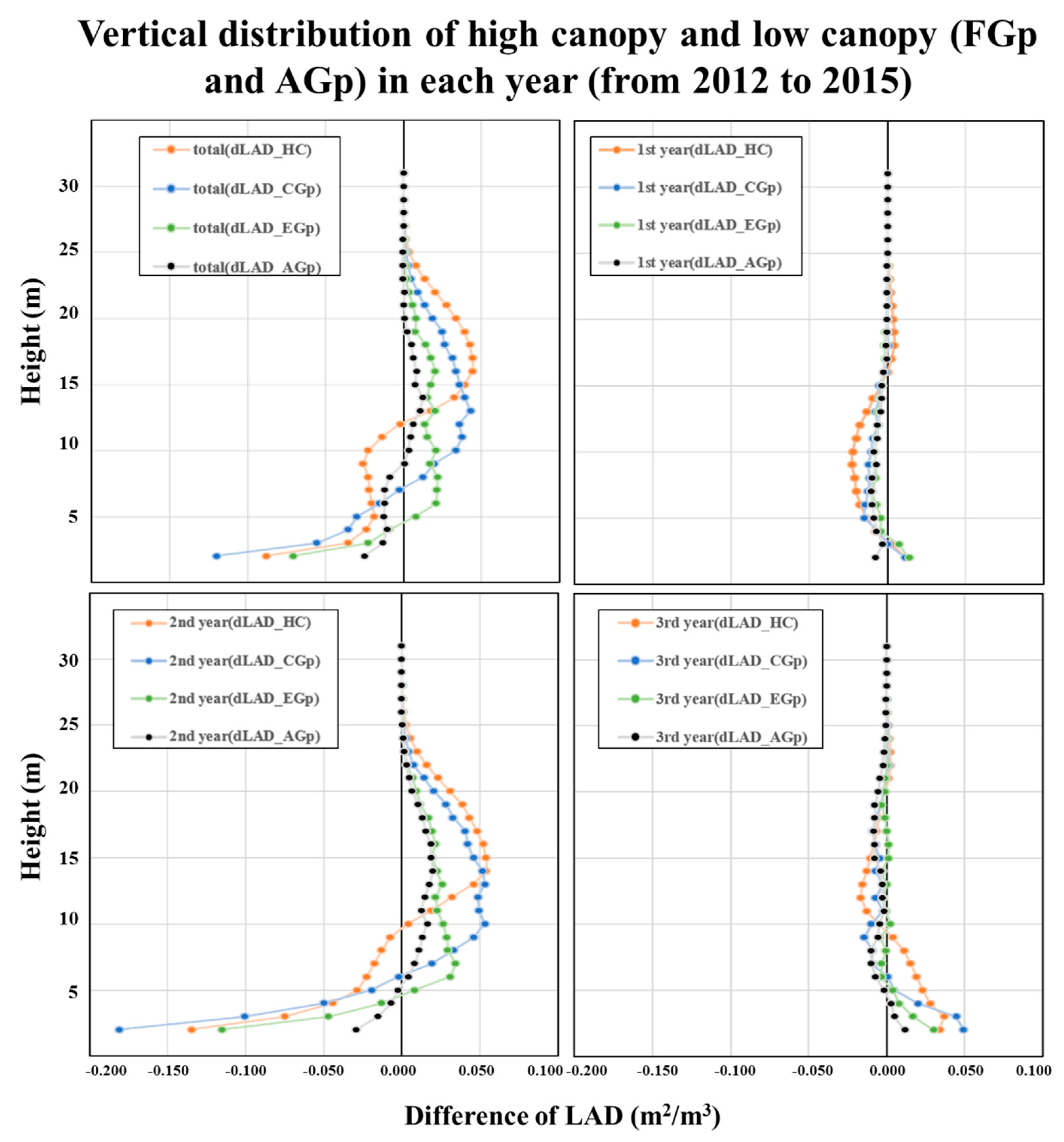
We also concluded that the leaf area index showed consistent values year by year, while the leaf area profile (e.g., leaf area density) showed inconsistent yearly changes in both high and low canopies. Among the low canopies, we could conclude that they were vulnerable to physical damage, particularly in AGps. In the case of FGps, they also drove the growth and disturbance aspects of forest dynamics and served to diversify the canopy structure; most of them were closing in a lateral direction by gap-edge trees. Furthermore, high canopies expanded their foliage at a higher height (12 m) than those of low canopies (5 m).
Spatial-temporal distribution and gap characteristics could provide key information about what state these structures are in (e.g., close to natural forest state) vertically and horizontally through comparison with other forests. Moreover, based on the gap types (i.e., natural or human-induced openings), our results could guide management priorities, such as designing a conservation area or planning a restoration, by giving comprehensive information on which parts of a forest are vulnerable to disturbances or require better, more efficient management.
Although we found that one-year interval change detections showed the potential to achieve detailed information about canopy changes, further study is warranted. For example, since detecting changes in the distribution of canopies might be easily affected by the grid size and the DOY of data acquisition, an adequate grid size and DOY should be suggested. In particular, in the case of DOY, seasonal variations in the canopies over a year could be studied with a mobile LiDAR, and this may both hint at the DOY of data acquisition via airborne LiDAR survey and inform about seasonal changes in canopy structures.

Funding

This work was supported by the National Research Foundation of Korea (NRF) grant funded by the Korea government (Ministry of Education) (No. NRF-2016R1D1A1B03933179)

Acknowledgments

This work was supported by the BK21 Plus Project in 2018 (Seoul National University Interdisciplinary Program in Landscape Architecture, Global leadership program towards innovative green infrastructure).

Conflicts of Interest

The authors declare no conflict of interest.

References

  1. Asner, G.P. Geography of forest disturbance. Proc. Natl. Acad. Sci. USA 2013, 110, 3711–3712. [Google Scholar] [CrossRef] [PubMed] [Green Version]
  2. Whitmore, T.C. Canopy Gaps and the Two Major Groups of Forest Trees. Ecology 1989, 70, 536–538. [Google Scholar] [CrossRef]
  3. Kane, V.R.; Gersonde, R.F.; Lutz, J.A.; McGaughey, R.J.; Bakker, J.D.; Franklin, J.F. Patch dynamics and the development of structural and spatial heterogeneity in Pacific Northwest forests. Can. J. For. Res. 2011, 41, 2276–2291. [Google Scholar] [CrossRef] [Green Version]
  4. Fisher, J.I.; Hurtt, G.C.; Thomas, R.Q.; Chambers, J.Q. Clustered disturbances lead to bias in large-scale estimates based on forest sample plots. Ecol. Lett. 2008, 11, 554–563. [Google Scholar] [CrossRef] [PubMed]
  5. Steenberg, J.W.; Millward, A.A.; Nowak, D.J.; Robinson, P.J. A conceptual framework of urban forest ecosystem vulnerability. Environ. Rev. 2016, 25, 115–126. [Google Scholar] [CrossRef]
  6. Vepakomma, U.D.; Kneeshaw, D.; De Grandpre, L. Influence of Natural and Anthropogenic Linear Canopy Openings on Forest Structural Patterns Investigated Using LiDAR. Forests 2018, 9. [Google Scholar] [CrossRef]
  7. Lee, D.K.; Kim, E.Y.; Song, W.K.; Park, C.; Choe, H.Y. Classification of Urban Forest Types and its Application Methods for Forests Creation and Management. J. Korea Soc. Environ. Restor. Technol. 2009, 12, 101–109. [Google Scholar]
  8. Kim, E.; Song, W.; Lee, D. A multi-scale metrics approach to forest fragmentation for Strategic Environmental Impact Assessment. Environ. Impact Assess. Rev. 2013, 42, 31–38. [Google Scholar] [CrossRef]
  9. Kim, K.-H.; Pauleit, S. Woodland changes and their impacts on the landscape structure in South Korea, Kwangju City Region. Landsc. Res. 2009, 34, 257–277. [Google Scholar] [CrossRef]
  10. Lee, J.-D.; Kim, M.-H. Development and practicability evaluation of GIS-based cemetery information management system. J. Korean Soc. Surv. Geod. Photogramm. Cartogr. 2010, 28, 223–231. [Google Scholar]
  11. Youn, Y.-C. Use of forest resources, traditional forest-related knowledge and livelihood of forest dependent communities: Cases in South Korea. For. Ecol. Manag. 2009, 257, 2027–2034. [Google Scholar] [CrossRef]
  12. Ryu, J.E.; Hwang, J.H.; Lee, J.H.; Chung, H.I.; Lee, K.I.; Choi, Y.Y.; Zhu, Y.; Sung, M.J.; Jang, R.; Sung, H.C.; et al. Analysis of Changes in Forest According to Urban Expansion Pattern and Morphological Features-Focused on Seoul and Daegu. Korean J. Remote Sens. 2017, 33, 835–854. [Google Scholar]
  13. Koo, J.-C.; Park, M.S.; Youn, Y.-C. Preferences of urban dwellers on urban forest recreational services in South Korea. Urban For. Urban Green. 2013, 12, 200–210. [Google Scholar] [CrossRef]
  14. Park, M.; Lee, H. Forest policy and law for sustainability within the Korean Peninsula. Sustainability 2014, 6, 5162–5186. [Google Scholar] [CrossRef]
  15. Sasaki, T.; Imanishi, J.; Ioki, K.; Song, Y.; Morimoto, Y. Estimation of leaf area index gap fraction in two broad-leaved forests by using small-footprint airborne, L.i.D.A.R. Landsc. Ecol. Eng. 2013, 12, 117–127. [Google Scholar] [CrossRef]
  16. Whitehurst, A.; Swatantran, A.; Blair, J.; Hofton, M.; Dubayah, R. Characterization of Canopy Layering in Forested Ecosystems Using Full Waveform Lidar. Remote Sens. 2013, 5, 2014–2036. [Google Scholar] [CrossRef] [Green Version]
  17. White, J.; Stepper, C.; Tompalski, P.; Coops, N.; Wulder, M. Comparing ALS and Image-Based Point Cloud Metrics and Modelled Forest Inventory Attributes in a Complex Coastal Forest Environment. Forests 2015, 6, 3704. [Google Scholar] [CrossRef]
  18. Thompson, I.D.; Maher, S.C.; Rouillard, D.P.; Fryxell, J.M.; Baker, J.A. Accuracy of forest inventory mapping: Some implications for boreal forest management. For. Ecol. Manag. 2007, 252, 208–221. [Google Scholar] [CrossRef]
  19. Magnussen, S.; Næsset, E.; Gobakken, T.; Frazer, G. A fine-scale model for area-based predictions of tree-size-related attributes derived from LiDAR canopy heights. Scand. J. For. Res. 2012, 27, 312–322. [Google Scholar] [CrossRef]
  20. Latifi, H.; Heurich, M.; Hartig, F.; Müller, J.; Krzystek, P.; Jehl, H.; Dech, S. Estimating over-and understorey canopy density of temperate mixed stands by airborne LiDAR data. For. Int. J. For. Res. 2016, 89, 69–81. [Google Scholar] [CrossRef]
  21. Naesset, E. Determination of mean tree height of forest stands using airborne laser scanner data. ISPRS 1997, 52, 49–56. [Google Scholar] [CrossRef]
  22. Andersen, H.-E.; Reutebuch, S.E.; McGaughey, R.J. A rigorous assessment of tree height measurements obtained using airborne lidar and conventional field methods. Can. J. Remote Sens. 2006, 32, 355–366. [Google Scholar] [CrossRef]
  23. Eitel, J.U.H.; Höfle, B.; Vierling, L.A.; Abellán, A.; Asner, G.P.; Deems, J.S.; Vierling, K.T. Beyond 3-D: The new spectrum of lidar applications for earth and ecological sciences. Remote Sens. Env. 2016, 186, 372–392. [Google Scholar] [CrossRef] [Green Version]
  24. Song, Y.; Imanishi, J.; Sasaki, T.; Ioki, K.; Morimoto, Y. Estimation of broad-leaved canopy growth in the urban forested area using multi-temporal airborne LiDAR datasets. Urban For. Urban Green. 2016, 16, 142–149. [Google Scholar] [CrossRef]
  25. Yu, X.; Hyyppa, J.; Kaartinen, H.; Maltamo, M.; Hyyppa, H. Obtaining plotwise mean height and volume growth in boreal forests using multi-temporal laser surveys and various change detection techniques. Int. J. Remote Sens. 2008, 29, 1367–1386. [Google Scholar] [CrossRef]
  26. Vepakomma, U.; St-Onge, B.; Kneeshaw, D. Spatially explicit characterization of boreal forest gap dynamics using multi-temporal lidar data. Remote Sens. Environ. 2008, 112, 2326–2340. [Google Scholar] [CrossRef]
  27. Vepakomma, U.; St-Onge, B.; Kneeshaw, D. Response of a boreal forest to canopy opening: Assessing vertical and lateral tree growth with multi-temporal lidar data. Ecol. Appl. 2011, 21, 99–121. [Google Scholar] [CrossRef]
  28. Vepakomma, U.; Kneeshaw, D.; Fortin, M.J. Spatial contiguity and continuity of canopy gaps in mixed wood boreal forests: Persistence, expansion, shrinkage and displacement. J. Ecol. 2012, 100, 1257–1268. [Google Scholar] [CrossRef]
  29. Zhao, K.; Suarez, J.C.; Garcia, M.; Hu, T.; Wang, C.; Londo, A. Utility of multitemporal lidar for forest and carbon monitoring: Tree growth, biomass dynamics, and carbon flux. Remote Sens. Environ. 2018, 204, 883–897. [Google Scholar] [CrossRef]
  30. Dalponte, M.; Jucker, T.; Liu, S.; Frizzera, L.; Gianelle, D. Characterizing forest carbon dynamics using multi-temporal lidar data. Remote Sens. Environ. 2019, 224, 412–420. [Google Scholar] [CrossRef]
  31. Cao, L.; Coops, N.C.; Innes, J.L.; Sheppard, S.R.J.; Fu, L.; Ruan, H.; She, G. Estimation of forest biomass dynamics in subtropical forests using multi-temporal airborne LiDAR data. Remote Sens. Environ. 2016, 178, 158–171. [Google Scholar] [CrossRef]
  32. Dalagnol, R.; Phillips, O.L.; Gloor, E.; Galvão, L.S.; Wagner, F.H.; Locks, C.J.; Aragão, L.E. Quantifying Canopy Tree Loss Gap Recovery in Tropical Forests under Low-Intensity Logging Using VHRSatellite Imagery Airborne, L.i.D.A.R. Remote Sens. 2019, 11, 817. [Google Scholar] [CrossRef]
  33. Rangel Pinagé, E.; Keller, M.; Duffy, P.; Longo, M.; dos-Santos, M.N.; Morton, D.C. Long-Term Impacts of Selective Logging on Amazon Forest Dynamics from Multi-Temporal Airborne LiDAR. Remote Sens. 2019, 11, 709. [Google Scholar] [CrossRef]
  34. Hopkinson, C.; Chasmer, L.; Hall, R.J. The uncertainty in conifer plantation growth prediction from multi-temporal lidar datasets. Remote Sens. Environ. 2008, 112, 1168–1180. [Google Scholar] [CrossRef]
  35. Ossola, A.; Hopton, M.E. Measuring urban tree loss dynamics across residential landscapes. Sci. Total Environ. 2018, 612 (Suppl. C), 940–949. [Google Scholar] [CrossRef]
  36. Bolund, P.; Hunhammar, S. Ecosystem services in urban areas. Ecol. Econ. 1999, 29, 293–301. [Google Scholar] [CrossRef]
  37. Lai, S.; Leone, F. Bridging biodiversity conservation objectives with landscape planning through green infrastructures: A case study from Sardinia, Italy. In Proceedings of the International Conference on Computational Science and Its Applications, Trieste, Italy, 3–6 July 2017. [Google Scholar]
  38. McWilliam, W.; Eagles, P.; Seasons, M.; Brown, R. Assessing the degradation effects of local residents on urban forests in Ontario, Canada. J. Arboric. 2010, 36, 253. [Google Scholar]
  39. Liu, Y.; Wang, Y.; Peng, J.; Du, Y.; Liu, X.; Li, S.; Zhang, D. Correlations between Urbanization and Vegetation Degradation across the World’s Metropolises Using DMSP/OLS Nighttime Light Data. Remote Sens. 2015, 7, 2067–2088. [Google Scholar] [CrossRef]
  40. Li, Y.; Kang, W.; Han, Y.; Song, Y. Spatial and temporal patterns of microclimates at an urban forest edge and their management implications. Environ. Monit. Assess. 2018, 190, 93. [Google Scholar] [CrossRef] [PubMed]
  41. Cumming, A.B.; Twardus, D.B.; Nowak, D.J. Urban forest health monitoring: Large-scale assessments in the United States. Aboricult. Urban For. 2008, 34, 341–346. [Google Scholar]
  42. Song, Y.; Ryu, Y. Seasonal changes in vertical canopy structure in a temperate broadleaved forest in Korea. Ecol. Res. 2015, 30, 821–831. [Google Scholar] [CrossRef]
  43. Yamamoto, S.-I. Forest gap dynamics and tree regeneration. J. For. Res. 2000, 5, 223–229. [Google Scholar] [CrossRef]
  44. Runkle, J.R. Guidelines and Sample Protocol for Sampling Forest Gaps; Pacific Northwest Research Station: Corvallis, OR, USA, 1992; Volume 283. [Google Scholar]
  45. Alexander, C.; Korstjens, A.H.; Hill, R.A. Influence of micro-topography and crown characteristics on tree height estimations in tropical forests based on LiDAR canopy height models. Int. J. Appl. Earth Obs. Geoinf. 2018, 65, 105–113. [Google Scholar] [CrossRef]
  46. Khosravipour, A.; Skidmore, A.K.; Wang, T.; Isenburg, M.; Khoshelham, K. Effect of slope on treetop detection using a LiDAR Canopy Height Model. ISPRS J. Photogramm. Remote Sens. 2015, 104, 44–52. [Google Scholar] [CrossRef]
  47. Roussel, J.-R.; Caspersen, J.; Béland, M.; Thomas, S.; Achim, A. Removing bias from LiDAR-based estimates of canopy height: Accounting for the effects of pulse density and footprint size. Remote Sens. Environ. 2017, 198, 1–16. [Google Scholar] [CrossRef]
  48. Zhang, Z.; Cao, L.; She, G. Estimating Forest Structural Parameters Using Canopy Metrics Derived from Airborne LiDAR Data in Subtropical Forests. Remote Sens. 2017, 9, 940. [Google Scholar] [CrossRef]
  49. Kellner, J.R.; Asner, G.P. Convergent structural responses of tropical forests to diverse disturbance regimes. Ecol. Lett. 2009, 12, 887–897. [Google Scholar] [CrossRef] [PubMed]
  50. Vaughn, N.R.; Asner, G.P.; Giardina, C.P. Long-term fragmentation effects on the distribution and dynamics of canopy gaps in a tropical montane forest. Ecosphere 2015, 6, 1–15. [Google Scholar] [CrossRef]
  51. Asner, G.P.; Kellner, J.R.; Kennedy-Bowdoin, T.; Knapp, D.E.; Anderson, C.; Martin, R.E. Forest Canopy Gap Distributions in the Southern Peruvian Amazon. PLoS ONE 2013, 8, 10. [Google Scholar] [CrossRef]
  52. Bouvier, M.; Durrieu, S.; Fournier, R.A.; Renaud, J.-P. Generalizing predictive models of forest inventory attributes using an area-based approach with airborne LiDAR data. Remote Sens. Environ. 2015, 156, 322–334. [Google Scholar] [CrossRef]
  53. Parker, G.G.; Harmon, M.E.; Lefsky, M.A.; Chen, J.; Pelt, R.V.; Weis, S.B.; Frankling, J.F. Three-dimensional Structure of an Old-growth Pseudotsuga-Tsuga Canopy and Its Implications for Radiation Balance, Microclimate, and Gas Exchange. Ecosystems 2004, 7, 440–453. [Google Scholar] [CrossRef]
  54. Jenness, J.S. Calculating landscape surface area from digital elevation models. Wildl. Soc. Bull. 2004, 32, 829–839. [Google Scholar] [CrossRef]
  55. Ishii, H.T.; Tanabe, S.; Hiura, T. Exploring the relationships among canopy structure, stand productivity, and biodiversity of temperature forest ecosystems. For. Sci. 2004, 50, 342–355. [Google Scholar]
  56. Jonckheere, I.; Fleck, S.; Nackaerts, K.; Muys, B.; Coppin, P.; Weiss, M.; Baret, F. Review of methods for in situ leaf area index determination. Agric. For. Meteorol. 2004, 121, 19–35. [Google Scholar] [CrossRef]
  57. Sasaki, T.; Imanishi, J.; Ioki, K.; Morimoto, Y.; Kitada, K. Estimation of leaf area index and canopy openness in broad-leaved forest using an airborne laser scanner in comparison with high-resolution near-infrared digital photography. Landsc. Ecol. Eng. 2008, 4, 47–55. [Google Scholar] [CrossRef]
  58. R Core Team. R: A Language and Rnvironment for Statistical Computing; R Foundation for Statistical Computing: Vienna, Austria, 2018. [Google Scholar]
  59. Kane, V.R.; McGaughey, R.J.; Bakker, J.D.; Gersonde, R.F.; Lutz, J.A.; Franklin, J.F. Comparisons between field- and LiDAR-based measures of stand structural complexity. Can. J. For. Res. 2010, 40, 761–773. [Google Scholar] [CrossRef]
  60. Valverde, T.; Silvertown, J. Canopy closure rate and forest structure. Ecology 1997, 78, 1555–1562. [Google Scholar] [CrossRef]
  61. St-Onge, B.; Vepakomma, U.; Sénécal, J.-F.; Kneeshaw, D.; Doyon, F. Canopy Gap Detection and Analysis with Airborne Laser Scanning. In Forestry Applications of Airborne Laser Scanning: Concepts and Case Studies; Maltamo, M., Næsset, E., Vauhkonen, J., Eds.; Springer: Dordrecht, The Netherlands, 2014; pp. 419–437. [Google Scholar]
Figure 1. Study site (boundary line) and eight airborne light detection and ranging (LiDAR) survey trajectories (red line). Artificial canopy openings or gaps: (a and b), sports facilities; (c and d), private graveyards; and (e and f), agricultural lands.
Remotesensing 11 01551 g001
Figure 2. Examples of open canopy scanned with mobile LiDAR. (a) Section view of an open canopy formed by a fallen tree. (b) Plane view of an open canopy (highlighted area).
Remotesensing 11 01551 g002
Figure 3. Analysis framework for the classification of urban open canopies in this study (a) and a section of a normalized LiDAR dataset (b) at an artificial gap (Figure 1c).
Remotesensing 11 01551 g003aRemotesensing 11 01551 g003b
Figure 4. Example of raster grids (height model) (a: 2015 canopy height model, 0.25 × 0.25 m2 resolution) and hexagon grids (height model) (b: 2015 normalized point cloud, 2.5 m edge length).
Remotesensing 11 01551 g004
Figure 5. Results from pixel-based analysis. (a) Distribution of high canopy (HC), low canopy (LC), canopy closure (CaC) from LC to HC, and damaged areas (2012–2015). (b) Distribution of growth and damaged areas in HCs. (c) Distribution of growth and damaged areas in LCs. (d) Distribution of growth areas in CaC; first year: 2012–2013, second year: 2013–2014, and third year: 2014–2015. DA: damaged area, VG: vertical growth area, and LG: lateral growth area.
Remotesensing 11 01551 g005aRemotesensing 11 01551 g005b
Figure 6. Plot-based canopy structure indices of HC and LC (forest gap and artificial gap). (a) Yearly leaf area index (LAI) for 2012–2015, (b) Yearly rumple index for 2012–2015
Remotesensing 11 01551 g006
Figure 7. Differences in leaf area density (LAD) (m2/m3) of high canopy and low canopy in each year from 2012 and 2015; dLAD_‘class’: differences between 2012 and 2015 in the canopy ‘class’; HC: high canopy; EGp: exiting gap; CGp: closed gap; AGp: artificial gap; total: between 2012 and 2015; first year: 2012–2013, second year: 2013–2014, and third year: 2014–2015; DA: damaged area, VG: vertical growth area, and LG: lateral growth area.
Remotesensing 11 01551 g007
Figure 8. Annual height decrements in high canopy and low canopy (FGp and AGp).
Remotesensing 11 01551 g008
Table 1. Examples of the canopy height model and hexagon height model
0.25 × 0.25 m2 Pixel-Level Height Model2.5 m Hexagon (16.24 m2) Plot-Level Height Model
ResultDistribution of vertical growth areaLeaf area density and leaf area index [52]
Distribution of lateral growth areaCanopy complexity [53,54]
Distribution of damaged areaPercentile height differences
ExamplePlease see Figure 4 below
Table 2. Annual mean vertical growth rate (unit: m/year) (first year: 2012–2013, second year: 2013–2014, and third year: 2014–2015; DA: damaged area, VG: vertical growth area, and LG: lateral growth area).
Canopy ClassPeriods (Terms)HMAX (Pixel)HMAX (Plot)H95TH (Plot)HMEAN (Plot)
HC to HCFirst year (218 days)0.290.250.250.29
Second year (396 days)0.300.300.290.32
Third year (401 days)0.290.290.290.30
Total years (1015 days)0.300.260.270.31
LC to LCFirst year (218 days)0.270.250.250.28
Second year (396 days)0.280.290.290.30
Third year (401 days)0.280.290.290.30
Total year (1015 days)0.270.270.270.30
Table 3. Correspondence of 3-year interval growth grids and annual continuous growth grids (A: growth pixels for 2012–2015, B: continuous growth pixels for 2012–2015).
LayersOverall Growth in the MidtermConsistent Growth through Short TermsConsistent Growth Area Ratio (%)
B:
A:(CHM2013 – CHM2012) > 0.1 mB/A × 100
(CHM2015 – CHM2012) > 0.1 mCHM2014 – CHM2013) > 0.1 m
CHM2015 – CHM2014) > 0.1 m
H95TH—hexagon grids (No. of hexagons)68,38126,57739
Hmax-pixel grids (No. of pixels)10,754,3511,706,38716
Table 4. Forest gap information (2012–2015).
Forest Gap 2012–2015
Year2012201320142015
No. of925792542601
λ (scaling exponent)1.281.261.281.28
Mean (m2)36 ± 9742 ± 10737 ± 8436 ± 70
Minimum (m2)10101010
Maximum (m2)225122121294906
Sum (m2)33,33533,51220,05821,361
Table 5. Existing gaps and closed gaps in forest gaps.
Forest Gap (FGp)Gap Continuation (Existing Gap, EGp)Closed Gap (CGp)
Year20122013201420152012–2015
No. of374363387391551
Mean (m2)65 ± 14770 ± 15346 ± 9746 ± 8516 ± 9
Minimum (m2)1010101010
Maximum (m2)22512212129490695
Sum (m2)24,27625,23717,85217,9079059
The difference in the number of existing gaps in each year might be due to gap coalescence (e.g., Vepakomma et al., [27]).
Table 6. Artificial gap area information (2012–2015).
Artificial Gap 2012–2015
Year2012201320142015
No. of607531540548
Mean (m2)237 ± 750280 ± 1,025226 ± 628246 ± 671
λ (scaling exponent)1.221.211.221.22
Minimum (m2)10101010
Maximum (m2)10,69418,7607,7137,736
Sum (m2)143,817148,666122,241134,935
Table 7. The ratio of open and closed areas by time (a) open or closed in the first year, (b) open or closed in the second year, (c) open or closed in the third year, (d) continuous changes to open to closed, and (e) total open or closed for 2012–2015, three-year term.
CategoriesOpen Area Ratio (%)Close Area Ratio (%)
Open or closed in the first year (a)3350
Newly open or closed in the second year (b)1429
Newly open or closed in the third year (c)6928
Opened (first year) → Closed (second year) → Opened (third year) or vice versa (d)157
Total (e: a + b + c − d)100100

