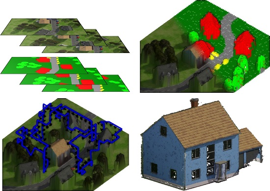
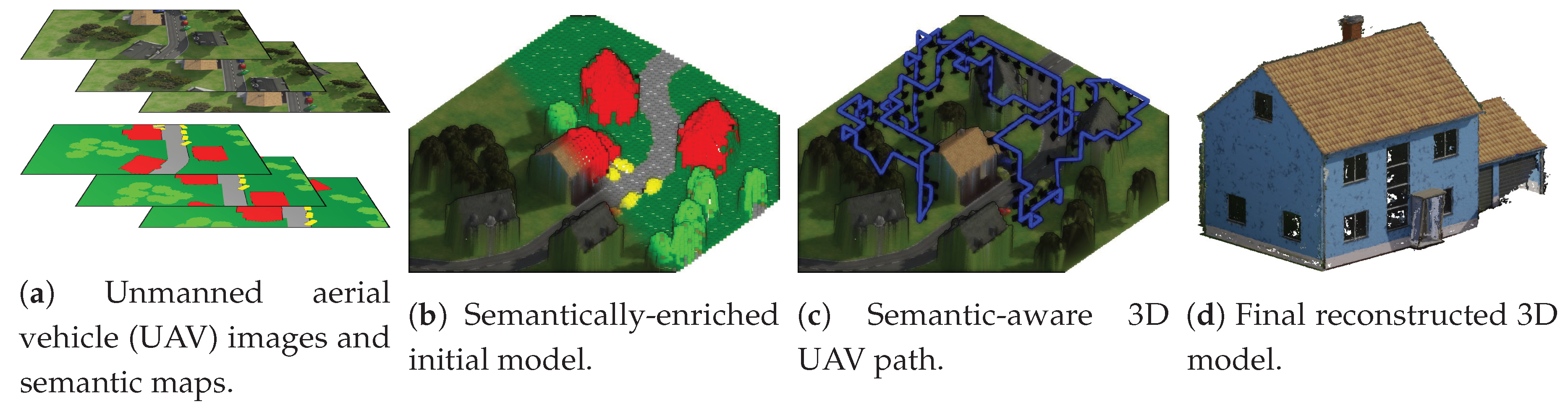
Automatic and Semantically-Aware 3D UAV Flight Planning for Image-Based 3D Reconstruction


Abstract
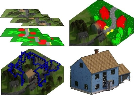
1. Introduction
- (1)
- We propose a set of heuristics based on photogrammetric reconstruction parameters, leading to individual flight paths for arbitrary camera intrinsics that ensure the generation of 3D models in a user-specified resolution.
- (2)
- We show how to exploit semantic segmentation of UAV imagery for extracting the target object and for generating a semantically-enriched initial 3D proxy model, which defines restricted and prohibited airspaces.
- (3)
- We propose a model-based optimization scheme with respect to a semantic model that maximizes the object coverage while minimizing the corresponding path length and avoiding restricted airspaces.
- (4)
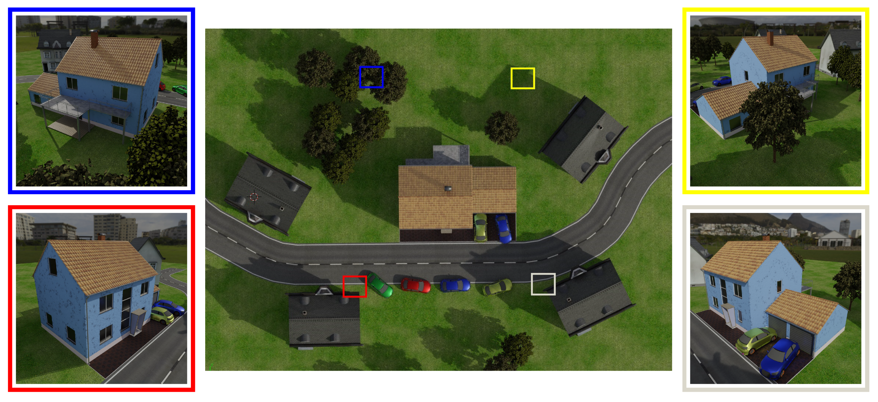
- We propose a realistic synthetic 3D model suitable for a comprehensive evaluation of urban flight planning, including a highly detailed building model embedded in a realistic and interchangeable scenery.
2. Related Work
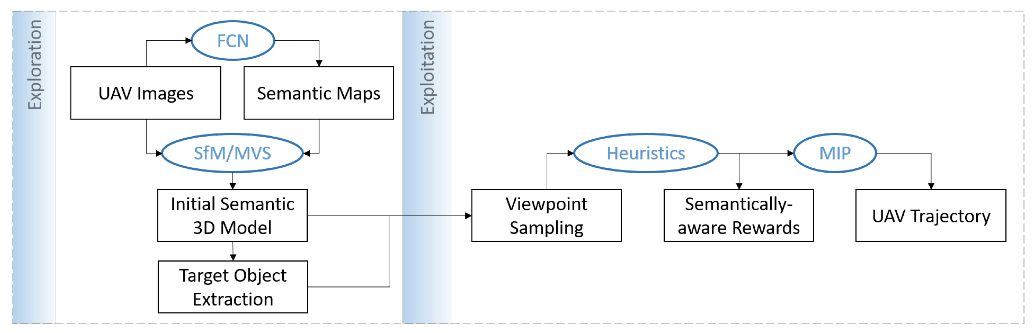
3. Proposed Flight Planning Pipeline
- Coverage: every point on the object surface has to be visible in at least two images to be able to triangulate its position in 3D space from the images.
- Safety: the estimated trajectory has to avoid collisions with obstacles and has to be aware of the semantics of the surrounding environment in terms of restricted and prohibited airspaces.
- Path length: the estimated trajectory should be as short as possible and avoid redundant views, as several images taken from similar camera poses introduce local uncertainties in depth estimation by glancing intersections.
- Heuristics: The estimated trajectory should facilitate complete reconstruction of the target object considering photogrammetric reconstruction criteria, such as GSD, observation angles, number of views, and sufficient overlap between adjacent views.
- Quality assessment: the path planning method should return an approximation of the expected reconstruction quality before the execution of the flight, in order to adjust the path or plan another subsequent path.
3.1. Notation and Definition of the Path Planning Problem
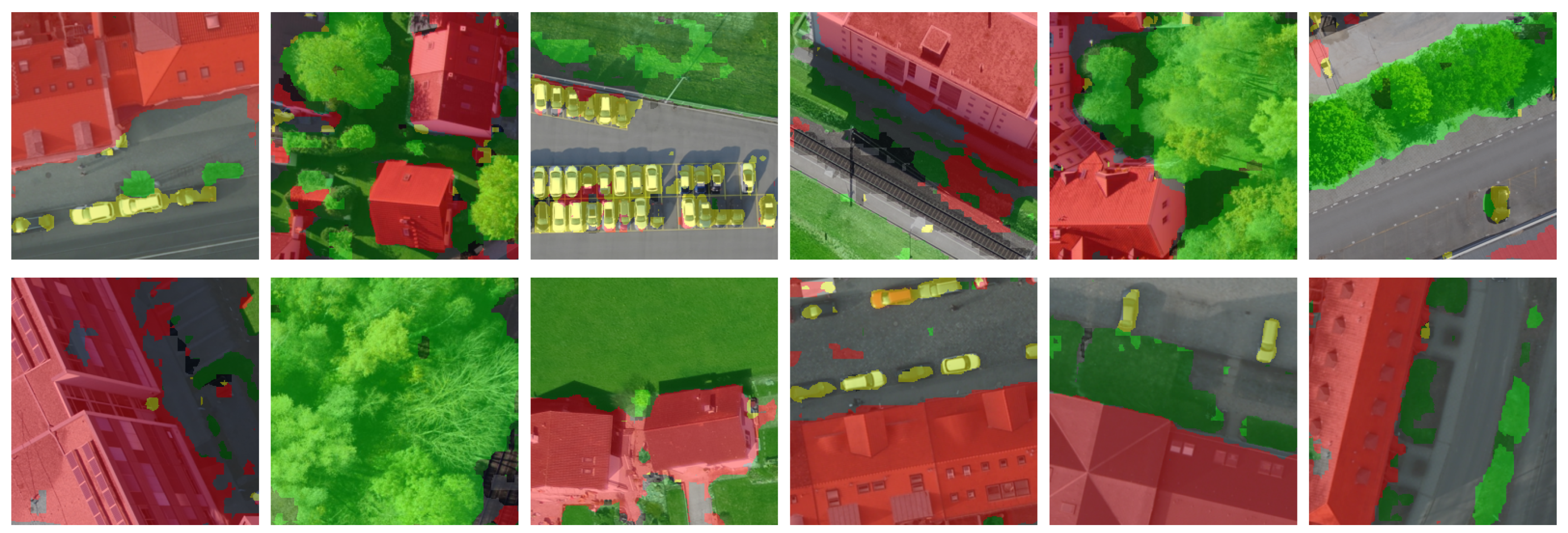
3.2. Semantically-Enriched Initial 3D Model
3.3. Camera Viewpoint Hypotheses Generation
3.4. Path Planning Heuristics
- (1)
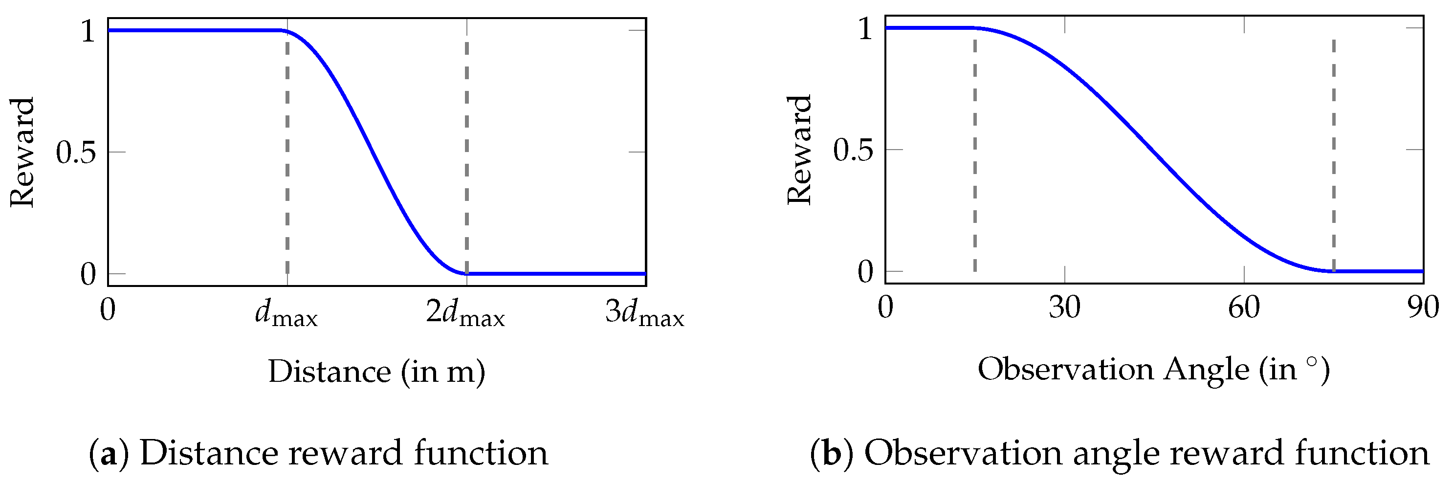
- Distance: the distance between camera viewpoints and object surface defines the resulting model resolution and depends on the desired point density and the camera intrinsics.
- (2)
- Observation angle: shallow observation angles between the camera views and surface normals are favored in MVS approaches.
- (3)
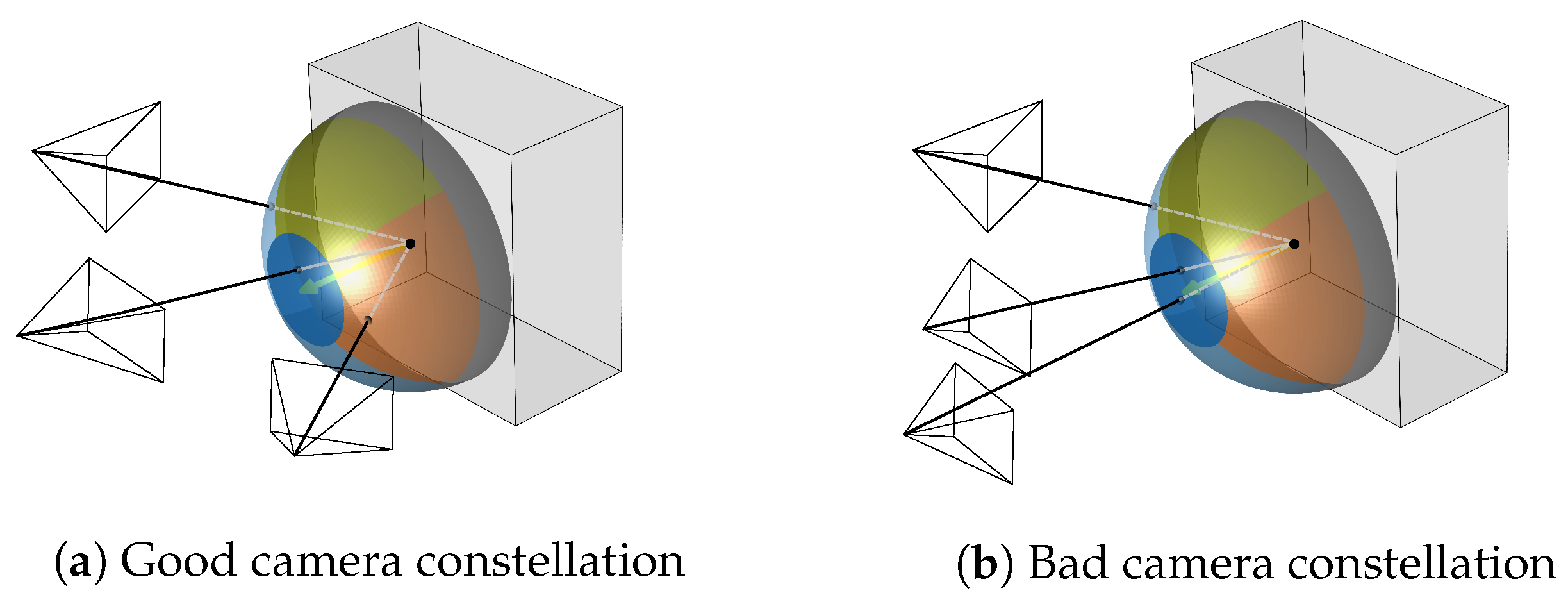
- Multiple views: every part of the scene has to be observed from at least two views from different perspectives with sufficient overlap between the views. The identification of corresponding points in overlapping images is the requirement for robustly estimating camera poses and for triangulating 3D object points.
- (4)
- Parallax angle: shallow parallax angles increase the triangulation error and therefore affect the model quality, while too large angles decrease the matchability between the views due to a lack of image similarity between the views which could result in a failure of the image registration step or in gaps in the reconstructed 3D model.
3.4.1. Distance
3.4.2. Observation Angle
3.5. Submodular Trajectory Optimization
| Algorithm 1 The greedy method for maximizing a monotone submodular function. | ||
| 1: | functionGreedy() | |
| 2: | compute | ▹ Compute individual rewards for all viewpoints |
| 3: | Seg compute | ▹ Compute intersection segments for all viewpoints |
| 4: | ▹ Initialize reconstructability of object | |
| 5: | ▹ Initialize observation directions of object | |
| 6: | for to do | |
| 7: | ||
| 8: | ||
| 9: | ||
| 10: | ||
| 11: | end for | |
| 12: | return | |
| 13: | end function | |
4. Experiments
4.1. Synthetic Scene
4.1.1. Optimization Evaluation
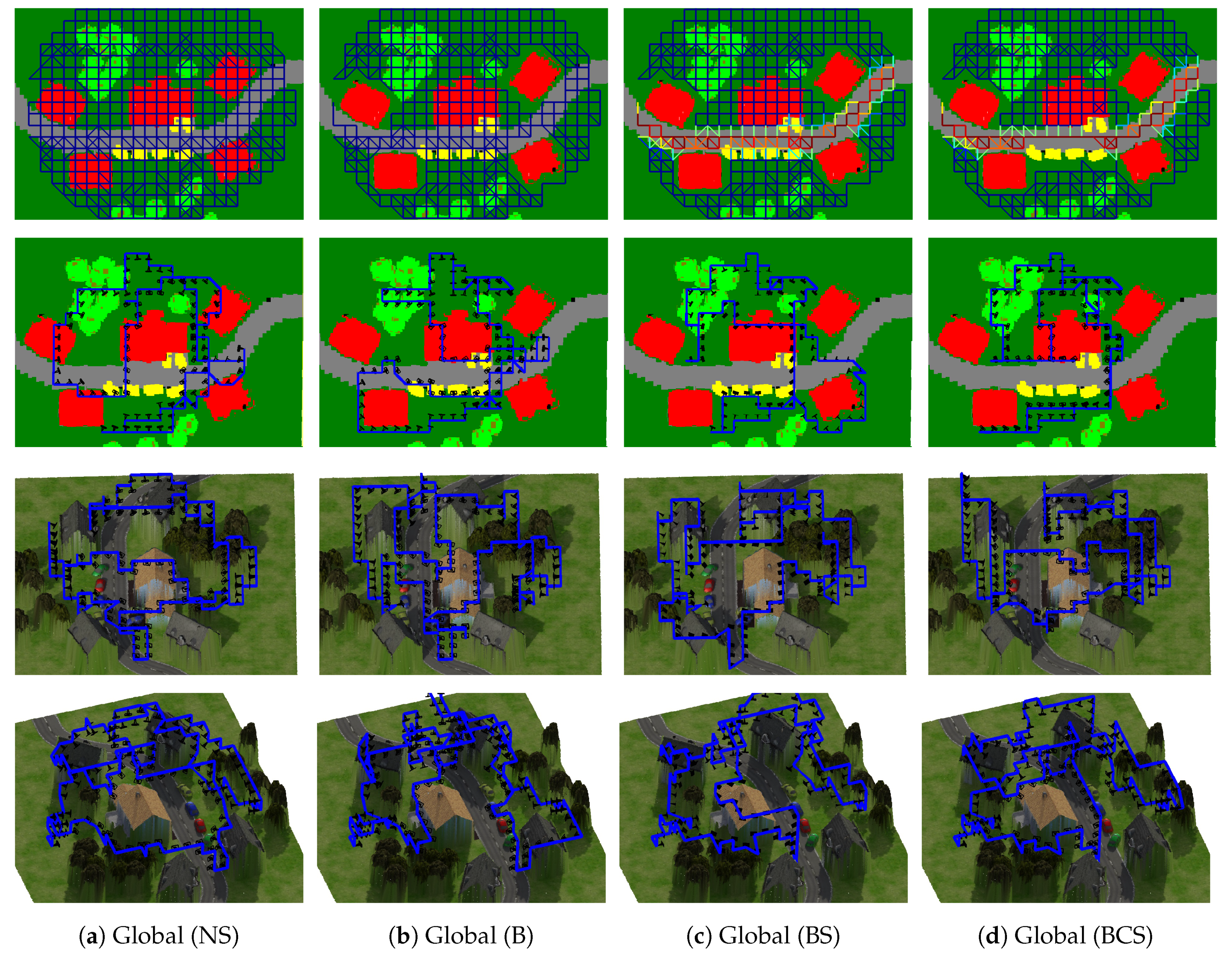
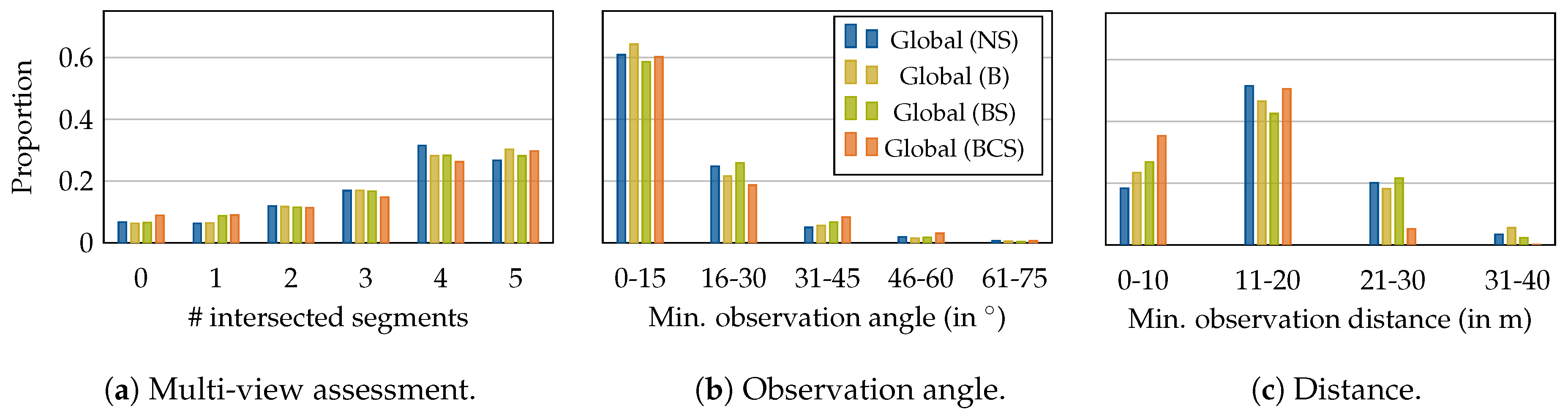
4.1.2. Semantically-Aware Optimization Evaluation
- No semantics (NS): this path from Section 4.1.1 serves as a baseline and only considers geometric constraints.
- Building (B): hard restriction for airspaces above other buildings than the target building.
- Building and Street (BS): in addition to (B), airspaces above streets are softly restricted to maximum path length of m, approximately twice the width of a regular street.
- Building, Car and Street (BCS): in addition to (BS), hard restrictions above cars are imposed.
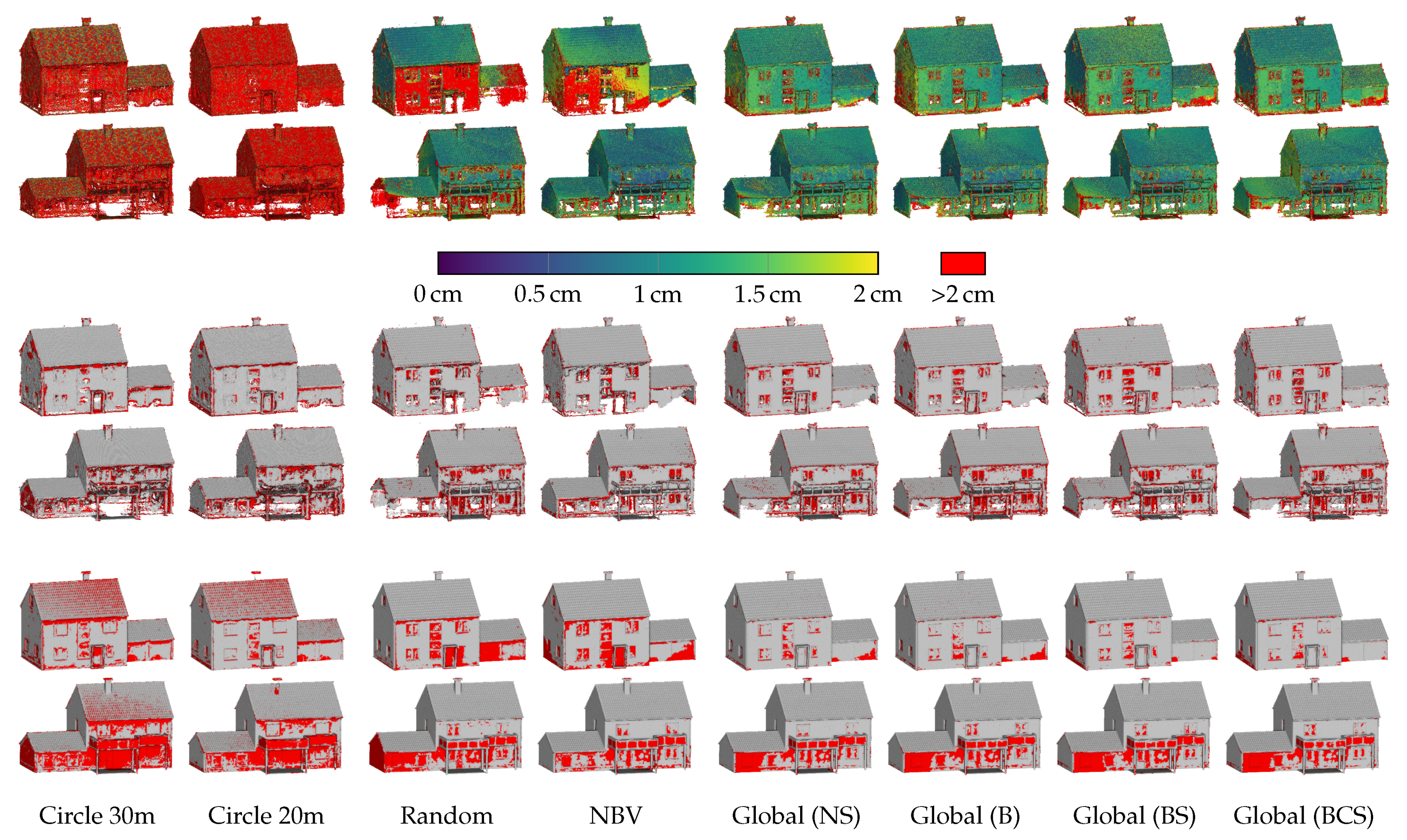
4.1.3. Reconstruction Performance
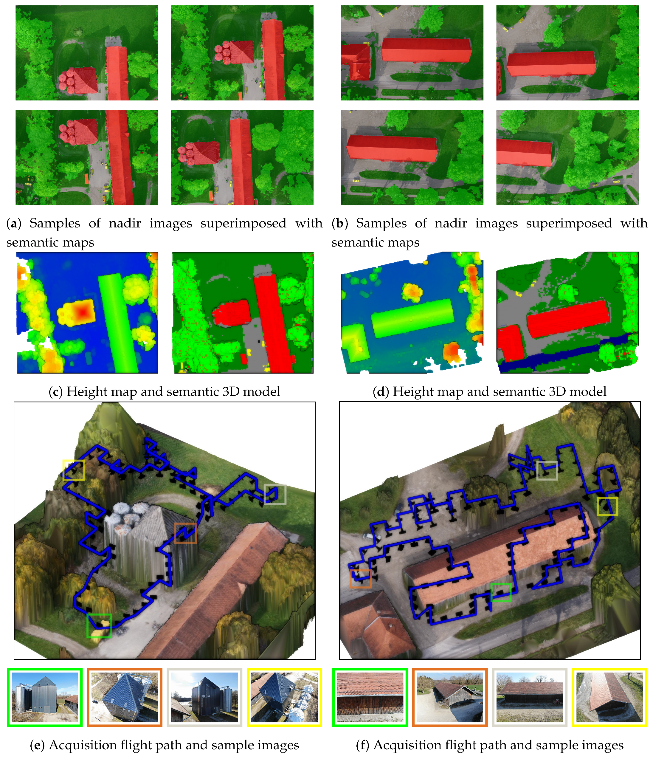
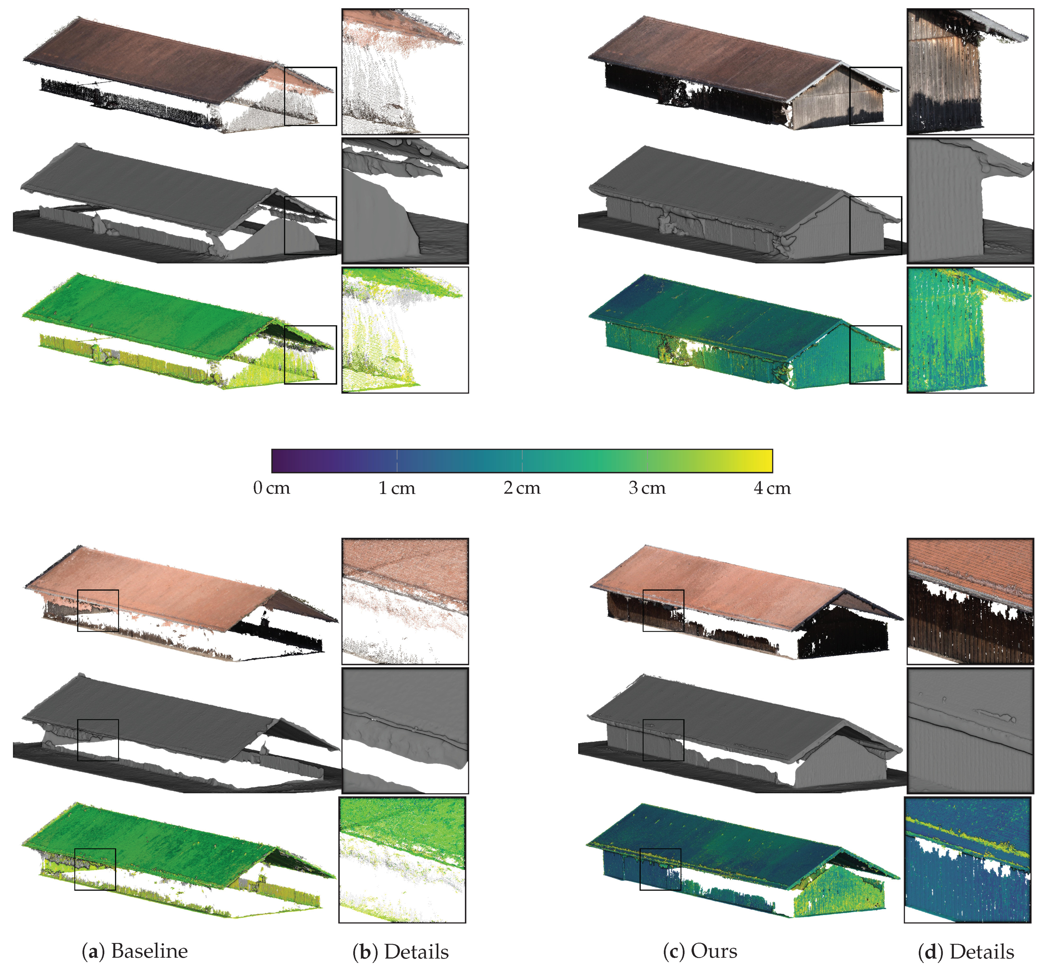
4.2. Real-World Performance
4.2.1. Silo
4.2.2. Farm
5. Conclusions
Author Contributions
Funding
Acknowledgments
Conflicts of Interest
References
- Pix4D: Pix4Dcapture. Available online: https://pix4d.com/product/pix4dcapture/ (accessed on 28 May 2019).
- Snavely, N.; Seitz, S.M.; Szeliski, R. Photo Tourism: Exploring Photo Collections in 3D. ACM Trans. Graph. 2006, 25, 835–846. [Google Scholar] [CrossRef]
- Schönberger, J.L.; Frahm, J.M. Structure-from-Motion Revisited. In Proceedings of the IEEE Conference on Computer Vision and Pattern Recognition (CVPR), Las Vegas, NV, USA, 27–30 June 2016. [Google Scholar]
- Vacanas, Y.; Themistocleous, K.; Agapiou, A.; Hadjimitsis, D. Building Information Modelling (BIM) and Unmanned Aerial Vehicle (UAV) Technologies in Infrastructure Construction Project Management and Delay and Disruption Analysis. In Proceedings of the International Conference on Remote Sensing and Geoinformation of the Environment, Paphos, Cyprus, 16–19 March 2015. [Google Scholar]
- Hallermann, N.; Morgenthal, G. Visual Inspection Strategies for Large Bridges using Unmanned Aerial Vehicles (UAV). In Proceedings of the 7th International Conference on Bridge Maintenance, Safety and Management (IABMAS), Shanghai, China, 7–11 July 2014; pp. 661–667. [Google Scholar]
- Mostegel, C.; Prettenthaler, R.; Fraundorfer, F.; Bischof, H. Scalable Surface Reconstruction from Point Clouds with Extreme Scale and Density Diversity. In Proceedings of the IEEE Conference on Computer Vision and Pattern Recognition (CVPR), Honolulu, HI, USA, 21–26 July 2017; pp. 904–913. [Google Scholar]
- Precisionhawk: Precision Flight. Available online: https://www.precisionhawk.com/precisionflight/ (accessed on 28 May 2019).
- DJI: Flight Planner. Available online: https://www.djiflightplanner.com/ (accessed on 28 May 2019).
- Ardupilot: Mission Planner. Available online: http://ardupilot.org/planner/ (accessed on 28 May 2019).
- Roberts, M.; Dey, D.; Truong, A.; Sinha, S.; Shah, S.; Kapoor, A.; Hanrahan, P.; Joshi, N. Submodular Trajectory Optimization for Aerial 3D Scanning. In Proceedings of the IEEE International Conference on Computer Vision (ICCV), Venice, Italy, 22–29 October 2017; pp. 5324–5333. [Google Scholar]
- Hepp, B.; Nießner, M.; Hilliges, O. Plan3D: Viewpoint and Trajectory Optimization for Aerial Multi-View Stereo Reconstruction. ACM Trans. Graph. 2018, 38, 4. [Google Scholar] [CrossRef]
- Cheng, P.; Keller, J.; Kumar, V. Time-optimal UAV Trajectory Planning for 3D Urban Structure Coverage. In Proceedings of the IEEE/RSJ International Conference on Intelligent Robots and Systems (IROS), Nice, France, 22–26 September 2008; pp. 2750–2757. [Google Scholar]
- Chakrabarty, A.; Langelaan, J. Energy Maps for Long-range Path Planning for Small-and Micro-UAVs. In Proceedings of the AIAA Guidance, Navigation, and Control Conference (GNC), Chicago, IL, USA, 10–13 August 2009; p. 6113. [Google Scholar]
- Di Franco, C.; Buttazzo, G. Coverage Path Planning for UAVs Photogrammetry with Energy and Resolution Constraints. J. Intell. Robot. Syst. 2016, 83, 445–462. [Google Scholar] [CrossRef]
- Zhu, X.X.; Tuia, D.; Mou, L.; Xia, G.S.; Zhang, L.; Xu, F.; Fraundorfer, F. Deep Learning in Remote Sensing: A Comprehensive Review and List of Resources. IEEE Geosci. Remote Sens. Mag. 2017, 5, 8–36. [Google Scholar] [CrossRef]
- Goesele, M.; Snavely, N.; Curless, B.; Hoppe, H.; Seitz, S.M. Multi-view Stereo for Community Photo Collections. In Proceedings of the IEEE International Conference on Computer Vision (ICCV), Rio de Janeiro, Brazil, 14–21 October 2007; pp. 1–8. [Google Scholar]
- Furukawa, Y.; Curless, B.; Seitz, S.M.; Szeliski, R. Towards Internet-scale Multi-view Stereo. In Proceedings of the IEEE Conference on Computer Vision and Pattern Recognition (CVPR), San Francisco, CA, USA, 13–18 June 2010; pp. 1434–1441. [Google Scholar]
- Rumpler, M.; Irschara, A.; Bischof, H. Multi-view Stereo: Redundancy Benefits for 3D Reconstruction. In Proceedings of the 35th Workshop of the Austrian Association for Pattern Recognition (AAPR), Graz, Austria, 26–27 May 2011. [Google Scholar]
- Furukawa, Y.; Hernández, C. Multi-view Stereo: A Tutorial. Found. Trends Comput. Graph. Vis. 2015, 9, 1–148. [Google Scholar] [CrossRef]
- Nex, F.; Remondino, F. UAV for 3D Mapping Applications: A Review. Appl. Geomat. 2014, 6, 1–15. [Google Scholar] [CrossRef]
- Kriegel, S.; Rink, C.; Bodenmüller, T.; Suppa, M. Efficient Next-best-scan Planning for Autonomous 3D Surface Reconstruction of Unknown Objects. J. Real-Time Image Process. 2015, 10, 611–631. [Google Scholar] [CrossRef]
- Heng, L.; Lee, G.H.; Fraundorfer, F.; Pollefeys, M. Real-time Photo-realistic 3D Mapping for Micro Aerial Vehicles. In Proceedings of the IEEE/RSJ International Conference on Intelligent Robots and Systems (IROS), San Francisco, CA, USA, 25–30 September 2011; pp. 4012–4019. [Google Scholar]
- Sturm, J.; Bylow, E.; Kerl, C.; Kahl, F.; Cremers, D. Dense Tracking and Mapping with a Quadrocopter. In Proceedings of the ISPRS—International Archives of the Photogrammetry, Remote Sensing and Spatial Information Sciences, XL-1/W2, Rostock, Germany, 4–6 September 2013; pp. 395–400. [Google Scholar]
- Loianno, G.; Thomas, J.; Kumar, V. Cooperative Localization and Mapping of MAVs using RGB-D Sensors. In Proceedings of the IEEE International Conference on Robotics and Automation (ICRA), Seattle, WA, USA, 26–30 May 2015; pp. 4021–4028. [Google Scholar]
- Michael, N.; Shen, S.; Mohta, K.; Kumar, V.; Nagatani, K.; Okada, Y.; Kiribayashi, S.; Otake, K.; Yoshida, K.; Ohno, K.; et al. Collaborative Mapping of an Earthquake Damaged Building via Ground and Aerial Robots. J. Field Robot. 2012, 29, 832–841. [Google Scholar] [CrossRef]
- Fan, X.; Zhang, L.; Brown, B.; Rusinkiewicz, S. Automated View and Path Planning for Scalable Multi-object 3D Scanning. ACM Trans. Graph. 2016, 35, 239. [Google Scholar] [CrossRef]
- Hepp, B.; Dey, D.; Sinha, S.N.; Kapoor, A.; Joshi, N.; Hilliges, O. Learn-to-Score: Efficient 3D Scene Exploration by Predicting View Utility. In Proceedings of the European Conference on Computer Vision (ECCV), Munich, Germany, 8–14 September 2018; pp. 437–452. [Google Scholar]
- Meng, Z.; Qin, H.; Chen, Z.; Chen, X.; Sun, H.; Lin, F.; Ang, M.H., Jr. A Two-Stage Optimized Next-View Planning Framework for 3-D Unknown Environment Exploration, and Structural Reconstruction. IEEE Robot. Autom. Lett. 2017, 2, 1680–1687. [Google Scholar] [CrossRef]
- Dunn, E.; Frahm, J.M. Next Best View Planning for Active Model Improvement. In Proceedings of the British Machine Vision Conference (BMVC), London, UK, 7–10 September 2009; pp. 1–11. [Google Scholar]
- Von Stumberg, L.; Usenko, V.; Engel, J.; Stückler, J.; Cremers, D. Autonomous Exploration with a Low-Cost Quadrocopter Using Semi-Dense Monocular SLAM. arXiv 2016, arXiv:1609.07835. [Google Scholar]
- Mendez, O.; Hadfield, S.; Pugeault, N.; Bowden, R. Taking the Scenic Route to 3D: Optimising Reconstruction from Moving Cameras. In Proceedings of the IEEE Conference on Computer Vision and Pattern Recognition (CVPR), Honolulu, HI, USA, 21–26 July 2017; Volume 3. [Google Scholar]
- Palazzolo, E.; Stachniss, C. Effective Exploration for MAVs Based on the Expected Information Gain. Drones 2018, 2, 9. [Google Scholar] [CrossRef]
- Kumar Ramakrishnan, S.; Grauman, K. Sidekick Policy Learning for Active Visual Exploration. In Proceedings of the European Conference on Computer Vision (ECCV), Munich, Germany, 8–14 September 2018; pp. 413–430. [Google Scholar]
- Border, R.; Gammell, J.D.; Newman, P. Surface Edge Explorer (SEE): Planning Next Best Views Directly from 3D Observations. In Proceedings of the IEEE International Conference on Robotics and Automation (ICRA), Brisbane, Australia, 21–25 May 2018; pp. 1–8. [Google Scholar]
- Hoppe, C.; Wendel, A.; Zollmann, S.; Pirker, K.; Irschara, A.; Bischof, H.; Kluckner, S. Photogrammetric Camera Network Design for Micro Aerial Vehicles. In Proceedings of the Computer Vision Winter Workshop (CVWW), Hernstein, Austria, 4–6 February 2012; Volume 8, pp. 1–3. [Google Scholar]
- Jing, W.; Polden, J.; Tao, P.Y.; Lin, W.; Shimada, K. View Planning for 3D Shape Reconstruction of Buildings with Unmanned Aerial Vehicles. In Proceedings of the IEEE International Conference on Control, Automation, Robotics and Vision (ICARCV), Phuket, Thailand, 13–15 November 2016; pp. 1–6. [Google Scholar]
- Smith, N.; Moehrle, N.; Goesele, M.; Heidrich, W. Aerial Path Planning for Urban Scene Reconstruction: A Continuous Optimization Method and Benchmark. In Proceedings of the ACM SIGGRAPH Asia, Tokyo, Japan, 4–7 December 2018; p. 183. [Google Scholar]
- Peng, C.; Isler, V. Adaptive View Planning for Aerial 3D Reconstruction of Complex Scenes. arXiv 2018, arXiv:1805.00506. [Google Scholar]
- Huang, R.; Zou, D.; Vaughan, R.; Tan, P. Active Image-based Modeling with a Toy Drone. In Proceedings of the IEEE International Conference on Robotics and Automation (ICRA), Brisbane, Australia, 21–25 May 2018; pp. 1–8. [Google Scholar]
- Alsadik, B.; Gerke, M.; Vosselman, G. Automated Camera Network Design for 3D Modeling of Cultural Heritage Objects. J. Cult. Herit. 2013, 14, 515–526. [Google Scholar] [CrossRef]
- Bircher, A.; Kamel, M.; Alexis, K.; Burri, M.; Oettershagen, P.; Omari, S.; Mantel, T.; Siegwart, R. Three-dimensional Coverage Path Planning via Viewpoint Resampling and Tour Optimization for Aerial Robots. Auton. Robot. 2016, 40, 1059–1078. [Google Scholar] [CrossRef]
- Snavely, N.; Seitz, S.M.; Szeliski, R. Skeletal Graphs for Efficient Structure from Motion. In Proceedings of the IEEE Conference on Computer Vision and Pattern Recognition (CVPR), Anchorage, AK, USA, 23–28 June 2008; Volume 1, pp. 1–8. [Google Scholar]
- Mostegel, C.; Rumpler, M.; Fraundorfer, F.; Bischof, H. UAV-based Autonomous Image Acquisition with Multi-view Stereo Quality Assurance by Confidence Prediction. In Proceedings of the IEEE Conference on Computer Vision and Pattern Recognition Workshops (CVPR-WS), Las Vegas, NV, USA, 26 June–1 July 2016; pp. 1–10. [Google Scholar]
- Devrim Kaba, M.; Gokhan Uzunbas, M.; Nam Lim, S. A Reinforcement Learning Approach to the View Planning Problem. In Proceedings of the IEEE Conference on Computer Vision and Pattern Recognition (CVPR), Honolulu, HI, USA, 21–26 July 2017; pp. 6933–6941. [Google Scholar]
- Marmanis, D.; Wegner, J.D.; Galliani, S.; Schindler, K.; Datcu, M.; Stilla, U. Semantic Segmentation of Aerial Images with an Ensemble of CNNs. ISPRS Ann. Photogramm. Remote Sens. Spat. Inf. Sci. 2016, 3, 473. [Google Scholar] [CrossRef]
- Kaiser, P.; Wegner, J.D.; Lucchi, A.; Jaggi, M.; Hofmann, T.; Schindler, K. Learning Aerial Image Segmentation from Online Maps. IEEE Trans. Geosci. Remote Sens. 2017, 55, 6054–6068. [Google Scholar] [CrossRef]
- Chen, K.; Fu, K.; Yan, M.; Gao, X.; Sun, X.; Wei, X. Semantic segmentation of aerial images with shuffling convolutional neural networks. IEEE Geosci. Remote Sens. Lett. 2018, 15, 173–177. [Google Scholar] [CrossRef]
- Wendel, A.; Maurer, M.; Graber, G.; Pock, T.; Bischof, H. Dense Reconstruction on-the-fly. In Proceedings of the IEEE Conference on Computer Vision and Pattern Recognition (CVPR), Providence, RI, USA, 16–21 June 2012; pp. 1450–1457. [Google Scholar]
- Long, J.; Shelhamer, E.; Darrell, T. Fully Convolutional Networks for Semantic Segmentation. In Proceedings of the IEEE Conference on Computer Vision and Pattern Recognition (CVPR), Providence, RI, USA, 16–21 June 2015; pp. 3431–3440. [Google Scholar]
- Semantic Drone Dataset. Available online: http://dronedataset.icg.tugraz.at (accessed on 28 May 2019).
- ISPRS 2D Semantic Labelling Contest—Potsdam. Available online: http://www2.isprs.org/commissions/comm3/wg4/2d-sem-label-potsdam.html (accessed on 28 May 2019).
- Katz, S.; Tal, A.; Basri, R. Direct Visibility of Point Sets. ACM Trans. Graph. 2007, 26, 24. [Google Scholar] [CrossRef]
- Hartley, R.; Zisserman, A. Multiple View Geometry in Computer Vision; Cambridge University Press: Cambridge, UK, 2003. [Google Scholar]
- Luhmann, T.; Robson, S.; Kyle, S.; Boehm, J. Close-Range Photogrammetry and 3D Imaging; Walter de Gruyter: Berlin, Germany, 2013. [Google Scholar]
- Förstner, W.; Wrobel, B.P. Photogrammetric Computer Vision; Springer: Berlin, Germany, 2016. [Google Scholar]
- Wenzel, K.; Rothermel, M.; Fritsch, D.; Haala, N. Image acquisition and model selection for multi-view stereo. ISPRS Arch. Photogramm. Remote Sens. Spat. Inf. Sci. 2013, 40, 251–258. [Google Scholar] [CrossRef]
- Kraus, K. Photogrammetry: Geometry from Images and Laser Scans; Walter de Gruyter: Berlin, Germany, 2011. [Google Scholar]
- Krause, A.; Golovin, D. Submodular Function Maximization; Cambridge University Press: Cambridge, UK, 2014. [Google Scholar]
- Blender Online Community. Blender—A 3D Modelling and Rendering Package; Blender Foundation, Blender Institute: Amsterdam, The Netherlands, 2018. [Google Scholar]
- Knapitsch, A.; Park, J.; Zhou, Q.Y.; Koltun, V. Tanks and Temples: Benchmarking Large-scale Scene Reconstruction. ACM Trans. Graph. 2017, 36, 78. [Google Scholar] [CrossRef]


| Dataset | Data Type | Extent of Building | Extent of Scene | Nr. of Nodes | Grid Spacing | Required GSD |
|---|---|---|---|---|---|---|
| (in m) | (in m) | (in m) | (in cm) | |||
| House | Synthetic | 2643 | 3 | 2.0 | ||
| Silo | Real | 2328 | 4 | 2.0 | ||
| Farm | Real | 1716 | 5 | 1.5 |
| Constraint | Nodes | Edges | ||
|---|---|---|---|---|
| Free | Restricted | Free | Restricted | |
| No semantics (NS) | 2643 | 0 | 13,634 | 0 |
| Building (B) | 2333 () | 0 | 11,836 () | 0 |
| Building and Street (BS) | 2333 () | 459 () | 11,836 () | 2555 () |
| Building, Car and Street (BCS) | 2208 () | 388 () | 11,084 () | 2164 () |
| Method | Images | Density (%) ↑ | Precision (%) ↑ | Completeness (%) ↑ | F-Score (%) ↑ | ||||
|---|---|---|---|---|---|---|---|---|---|
| GSD | 1.5GSD | ||||||||
| Circle 30 m | 100 | 46.9 | 73.3 | 88.8 | 96.3 | 79.2 | 91.8 | 83.7 | 94.0 |
| Circle 20 m | 100 | 29.7 | 60.3 | 89.7 | 95.8 | 84.0 | 93.9 | 86.7 | 94.8 |
| Random | 321 | 94.1 | 98.9 | 96.4 | 98.6 | 83.3 | 91.0 | 89.4 | 94.6 |
| Greedy NBV | 323 | 96.9 | 99.8 | 96.8 | 98.7 | 86.5 | 92.7 | 91.4 | 95.6 |
| Global (NS) | 148 | 97.6 | 99.9 | 96.7 | 98.9 | 91.1 | 95.7 | 93.8 | 97.2 |
| Global (B) | 162 | 97.3 | 99.8 | 96.2 | 98.7 | 88.3 | 95.5 | 92.1 | 97.1 |
| Global (BC) | 148 | 97.6 | 99.8 | 96.4 | 98.7 | 89.4 | 94.8 | 92.8 | 96.7 |
| Global (BCS) | 152 | 97.3 | 99.8 | 96.5 | 98.8 | 87.7 | 95.1 | 91.9 | 96.9 |
| Dataset | Baseline | Optimized | ||||||
|---|---|---|---|---|---|---|---|---|
| Images | Restricted | Path | Density | Images | Restricted | Path | Density | |
| Viewpoints | Length () | (cm) | Viewpoints | Length () | (cm) | |||
| Silo | 90 | 24 | 184 | 2.2 ± 1.2 | 98 | 0 | 405 | 2.0 ± 0.9 |
| Farm | 89 | 23 | 732 | 2.3 ± 0.8 | 131 | 0 | 677 | 0.9 ± 0.4 |
© 2019 by the authors. Licensee MDPI, Basel, Switzerland. This article is an open access article distributed under the terms and conditions of the Creative Commons Attribution (CC BY) license (http://creativecommons.org/licenses/by/4.0/).
Share and Cite
Koch, T.; Körner, M.; Fraundorfer, F. Automatic and Semantically-Aware 3D UAV Flight Planning for Image-Based 3D Reconstruction. Remote Sens. 2019, 11, 1550. https://doi.org/10.3390/rs11131550
Koch T, Körner M, Fraundorfer F. Automatic and Semantically-Aware 3D UAV Flight Planning for Image-Based 3D Reconstruction. Remote Sensing. 2019; 11(13):1550. https://doi.org/10.3390/rs11131550
Chicago/Turabian StyleKoch, Tobias, Marco Körner, and Friedrich Fraundorfer. 2019. "Automatic and Semantically-Aware 3D UAV Flight Planning for Image-Based 3D Reconstruction" Remote Sensing 11, no. 13: 1550. https://doi.org/10.3390/rs11131550
APA StyleKoch, T., Körner, M., & Fraundorfer, F. (2019). Automatic and Semantically-Aware 3D UAV Flight Planning for Image-Based 3D Reconstruction. Remote Sensing, 11(13), 1550. https://doi.org/10.3390/rs11131550