An Efficient In-Situ Debris Flow Monitoring System over a Wireless Accelerometer Network

Abstract

Debris flow disasters pose a serious threat to public safety in many areas all over the world, and it may cause severe consequences, including losses, injuries, and fatalities. With the emergence of deep learning and increased computation powers, nowadays, machine learning methods are being broadly acknowledged as a feasible solution to tackle the massive data generated from geo-informatics and sensing platforms to distill adequate information in the context of disaster monitoring. Aiming at detection of debris flow occurrences in a mountainous area of Sakurajima, Japan, this study demonstrates an efficient in-situ monitoring system which employs state-of-the-art machine learning techniques to exploit continuous monitoring data collected by a wireless accelerometer sensor network. Concretely, a two-stage data analysis process had been adopted, which consists of anomaly detection and debris flow event identification. The system had been validated with real data and generated favorable detection precision. Compared to other debris flow monitoring system, the proposed solution renders a batch of substantive merits, such as low-cost, high accuracy, and fewer maintenance efforts. Moreover, the presented data investigation scheme can be readily extended to deal with multi-modal data for more accurate debris monitoring, and we expect to expend addition sensory measurements shortly.

1. Introduction

Debris flow is a generic term describing the geological hazard that a large volume of a highly concentrated viscous water–debris mixture rapidly flows downward of the hillslope. The phenomena cause considerable damage throughout the world because it happens all of a sudden, destroys all objects in the paths, and often strikes without a sign. Extensive research efforts have been carried out to investigate debris flow from various aspects, such as material properties, movement mechanism, and velocity [1], to achieve better disaster prevention and management. As a result, the most widely accepted classification of debris flow has been developed [2], which expresses debris flow as a sediment mixture of rocks, mud, and water flows rapidly flush a gully bed. Mountainous regions in Japan are susceptible to debris flows, owing to the geographical features [3]. According to the report of Ministry of Land, Infrastructure, Transport, and Tourism of Japan (MLIT), debris flow counts had almost doubled over the past decade, i.e., jumped from 154 to 305 counts per year, which has caused considerable loss of life and property [4]. Moreover, this trend is anticipated to continue in the future attribute to the urbanization process and abrupt climate change. As a result, in line with the demand for disaster risk management, development of debris flow monitoring and early warning systems had been a long-standing and challenging research theme through decades in Japan [5].

The ultimate objective of debris flow monitoring is to make time for taking practical actions such as road closures and evacuations before disaster strikes the hazardous areas. Nowadays, debris flow monitoring systems can be generally subdivided into two classes: 1. Pre-event warning systems and in-progress early detection system.s The first category commonly performs statistical modeling over geographic information system (GIS) data, including air, land and many other climate related observations to predict the debris flow occurrence [6]. A warning would be issued while the estimate exceeds a certain threshold before debris flow arrival. 2. On the other hand, it is commonly based on another group of sensors installed onsite; and the system is designated to process the streaming data in (near) real-time and raise the alarm immediately once debris flow being detected [7]. Clearly, a pre-event warning system can win more time to avert the disaster. Nevertheless, the latter in-situ monitoring system is superior due to lower false alarm rates.

Currently, with the aid of advanced machine learning and the Internet-of-Things (IoT), more attention has been drawn to in-progress monitoring which allows immediate/dynamic disaster information reporting to public safety officials and local inhabitant. An overview diagram of in-situ debris flow monitoring system is shown in Figure 1, which commonly includes monitoring data collection/transmission hardware and a data analysis unit for debris flow event detection. A comprehensive set of sensors, such as rain gauge [8], X-band MP Rader, geophone [9], ultrasonic water level transmitter [10], wired sensor [11], had been evaluated for the task. The sensors are usually installed along the mountain slopes to capture debris flow-induced variations exhibited in the measurements. Robust communications is another critical part that enables the collection of streaming data. Wireless sensor network (WSN) is acknowledged as a viable solution according to the latest literature [11,12]. Subsequently, statistical machine learning algorithms are employed to analyze the captured sensory data to discern specific pattern arises by debris flow. The storage and processing of large volumes of monitoring data are perhaps the biggest challenges throughout system development [13]. Advancements in computing hardware and statistical machine learning algorithms have given rise to possible solutions to characterize the massive sensory data and generate decision supports in (near) real-time [14]. Concretely, data mining tools and techniques commonly convert the raw sensor data into a compressed representation with significant information well retained, such as summary statistics derived from time-series data [15], and Fourier and Wavelet spectrograms extraction for image/audio data [16]. At debris flow detection stage, various statistical machine learning techniques have been adopted to exploit the particular debris flow-induced patterns with the extracted feature representations, including support vector machine (SVM) [17], decision trees [18], and artificial neural networks (ANN) [19]. According to empirical studies, advanced machine learning methods are deemed to be well suited to handle the multivariate sensor data, which usually exhibits wide variability and complex non-linear distributions [20].

This study aims at developing an in-situ debris flow monitoring system which integrates advanced machine learning techniques to process massive data captured by the wireless accelerometer network. We summarize the key features of the proposed debris flow monitoring network as follows.

†Hardware design. Sensors play a vital role in debris flow monitoring. This study presents a novel design of vibration sensing device which equipped with a triaxial sensor, self-contained power unit with a rechargeable battery and solar panel, and the wireless communication unit. All components are available on the open market, and thus, the total price of one sensing unit is lower than 100 dollars. In the debris monitoring network design, we deployed 20 sensors covering a hazardous area of Nojiri river No.7 dam at Sakurajima, Japan. Through a wireless network, the sensing data were transmitted to a remote computer for further event-based investigation. The total hardware cost is substantially lower compared to other existed methods, such as wire sensor which demands high expense on wiring installation and maintenance. Section 3.1 presents the details related to hardware development.

†Data investigation framework. To deal with massive sensor data efficiently, we proposed a two-stage data processing flow, including anomaly detection phase and debris flow induced pattern identification phase. The first stage is designated to screen out a large volume of monitoring data contains no intensive dynamics induced by environmental hazards. It is noteworthy that there exists one critical issue that heavy rain and strong wind can arise significant displacement of accelerometers in addition to debris. To suppress false alarms, we perform a further investigation on the ‘suspicious’ data by using a deep learning algorithm to characterize the specific data patterns generated by debris flow. To our best knowledge, it is the first attempt to introduce deep learning technique to debris flow monitoring.

†Accelerometer data fusion. The above-introduced monitoring data gathering and analysis process work in parallel on every channel of sensor output. Aggregation of multi-sensor data turns out to be an efficient way to achieve more accurate and robust disaster monitoring. To this end, we proposed a multi-sensor information fusion scheme, and the details are shown in Section 3.2.4.

The paper is structured as follows: Section 2 provides an introduction to studied area and disaster background. Section 3 introduces sensing hardware design and data investigation framework for debris monitoring. Next, Section 4 and Section 5 outline the results of the case study with discussions. Finally, Section 6 presents the concluding remarks.

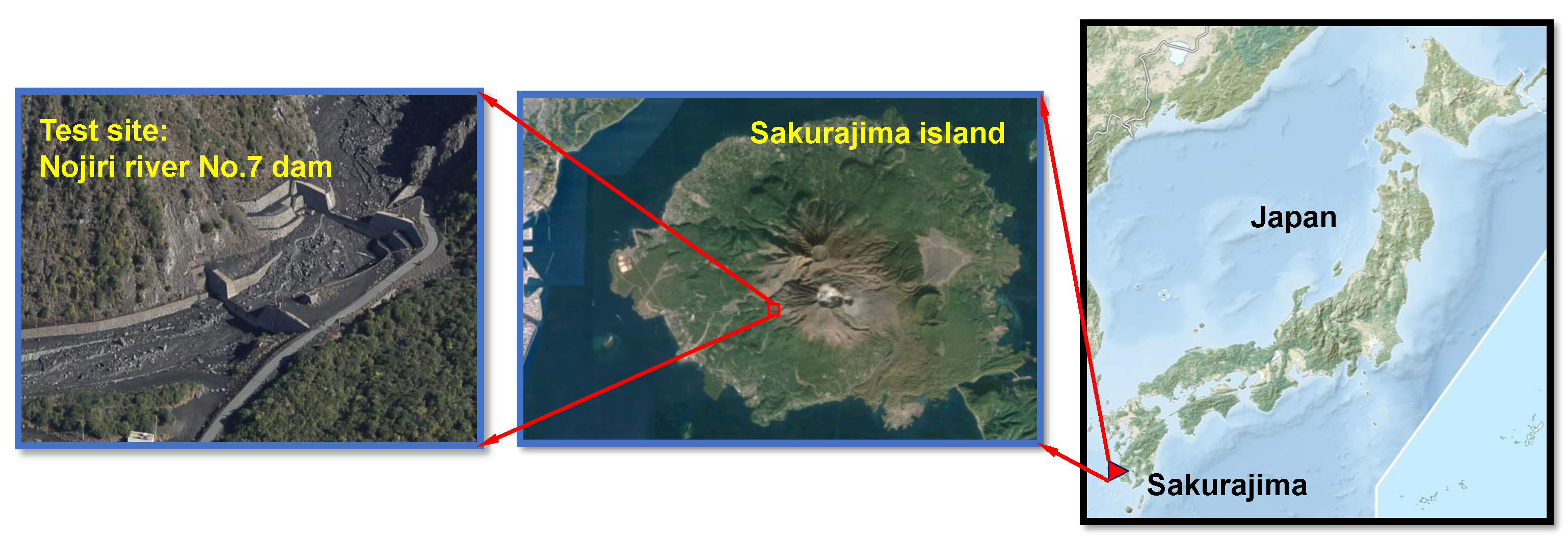
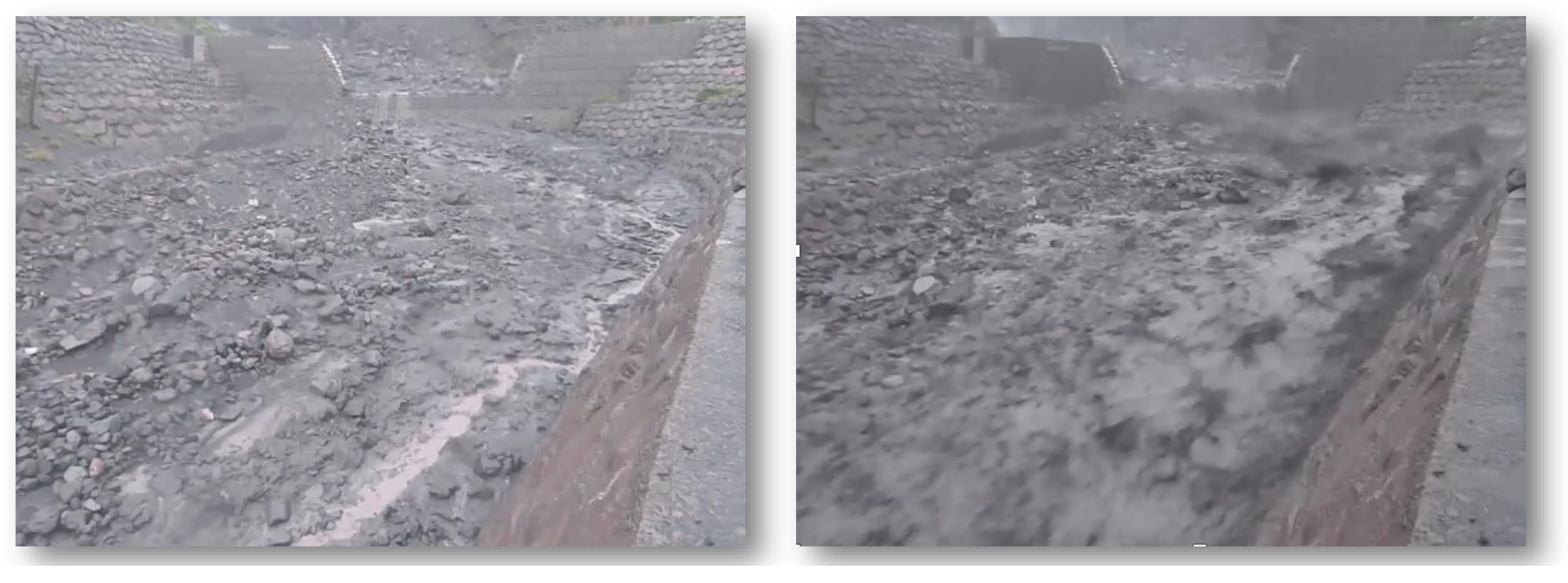
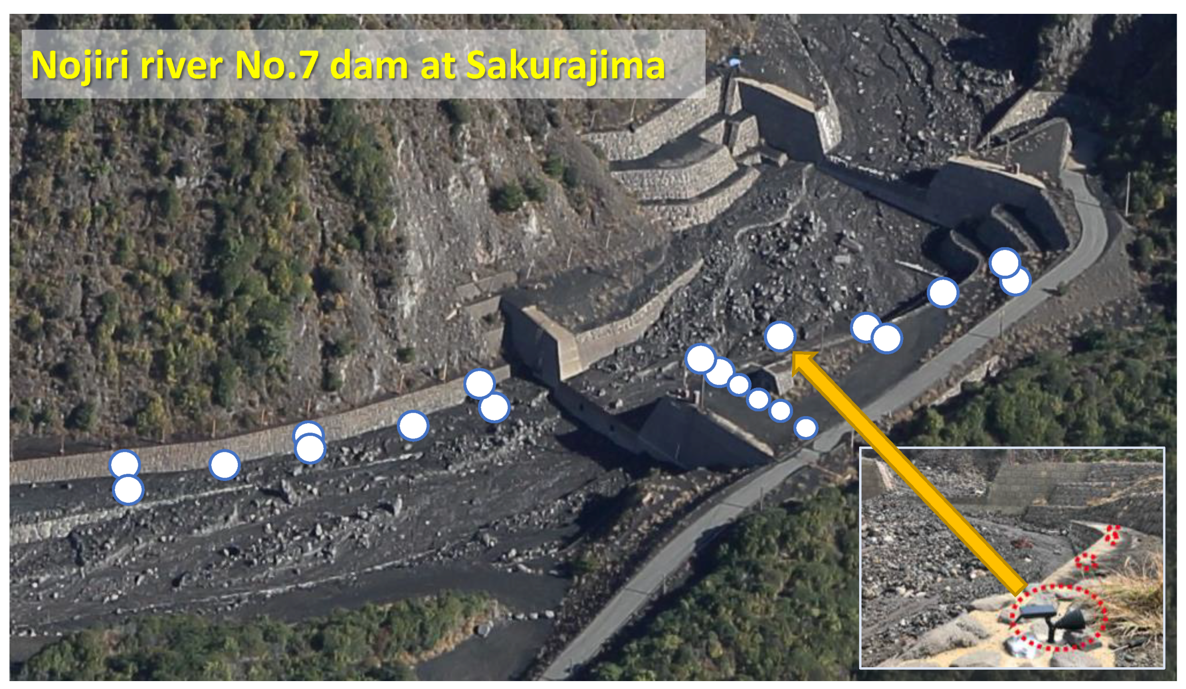
2. Overview of the Study Area

The study area is located in a mountainous region near Nojiri river No.7 dam of Sakurajima, which is an active volcano situated at 31${}^{\circ }$35${}^{\prime }$ N, 130${}^{\circ }$30${}^{\prime }$ E in the southern tip of Kyushu Island, Japan and we present an overview of the area in Figure 2. Sakurajima is 12 km long in the east–west direction and 9 km wide from north to south. It is a land-connected island with an area of about 80 km${}^2$ and the circumference of 50 km. A particular characteristic of Sakurajima’s debris flows is that the presence of large volumes of accumulated volcanic ash on the steep mountain slopes results in many debris-flow disasters even when only a small amount of rainfall occurs. There had been plenty of efforts devoted to managing the risk of debris flow at Sakurajima, such as deployment of multiple monitoring sensors including wire sensor, optical sensor, and the acoustic sensor for the disaster detection. Meanwhile, surveillance camera monitoring and mud-sampling are carried out as routine operations [5]. This study attempts to devise a low-cost monitoring system while retaining high accuracy in debris flow detection. Figure 3 shows two surveillance camera snapshots depicting the situation of non-hazardous and debris flow strikes, respectively. It can be seen that even the rain is not very heavy, volcanic ash piled on the steep mountain slopes is easily tuned to debris flow and traveled downhill to small basin areas.

3. Materials and Methods

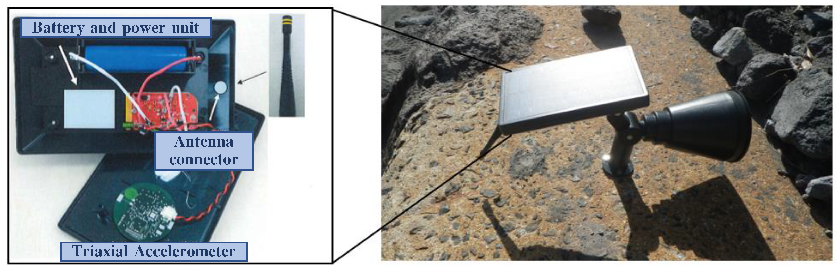
3.1. Design and Implementation of the Debris Flow Monitoring System Hardware

In this section, we demonstrate the sensing hardware system which lays the fundamentals of this research, which consists of three major parts: triaxial vibration sensor design, sensor deployment scheme over the monitoring area of Nojiri river No.7 high dam, and, wireless communication system settings.

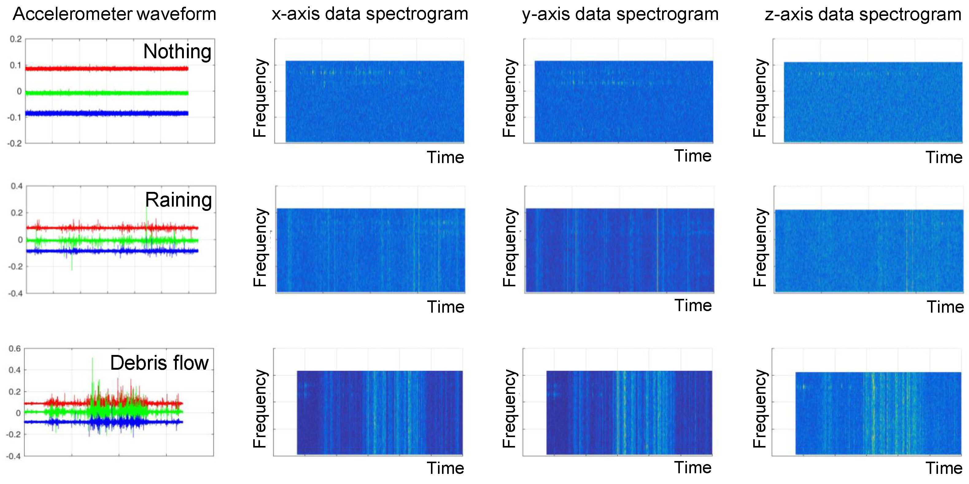
3.1.1. Triaxial Accelerometer Sensing Unit

Figure 4 illustrates the internal design of accelerometer implemented through this study, which is composed of three major components. We introduce those the detail of each part as follows. The power supply has been a long-lasting issue, especially for monitoring systems. In the current design, we expect the system to operate in a self-contained manner with the battery and solar power generator equipped. To this end, three standard 18,650 lithium batteries were used, which reach up to 40 Wh total capacity; meanwhile, we equipped a solar panel rated at 1.5 kWh per day. The operation power consumption is 10 mW, and thus, a vibration sensing unit can work continuously up to two weeks after fully charged. The selection of triaxial vibration sensor is another critical matter to the hardware system. We choose ADXL312 accelerometer developed at Analog Device Inc. At the wireless data transmission stage, we set the carrier band to 920 MHz with GFSK modulation mode. The sampling frequency was fixed to 50 Hz, which had been proved to be reliable for real-time data transmission even under hostile environment conditions.

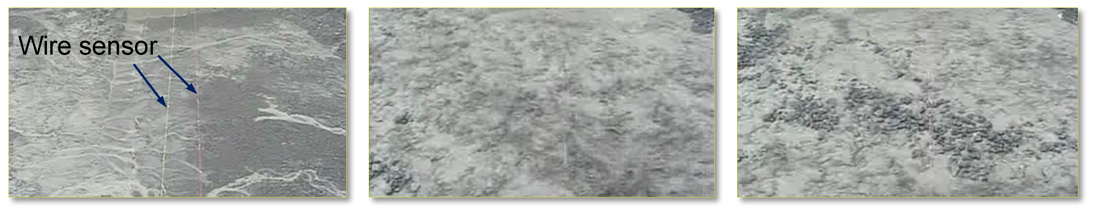
3.1.2. Sensor Deployment Map

In the system design, debris flow monitoring is performed over an accelerometer network with a series of distributed sensing nodes, each of which has data capture and communication capabilities. Since the accelerometer unit dedicated to this task is not pricey, we are able to distribute a batch of sensor nodes to achieve full coverage of the terrain monitored for regional vibration information characterization. It is noteworthy that the positions of nodes can significantly affect vibration observation, such as sensors located in a high place are more vulnerable to wind and rain effects. Based on this consideration, we placed sensing units at both high or low places along the dam tunnel to capture specific vibrations arise by debris flow progress and suppress environmental noises as well. The detailed installation map is shown in Figure 5.

Figure 6 shows examples of 5 min vibration data clips collected by monitoring accelerometer networks regarding environmental conditions. It is evident that the patterns, i.e., waveforms (first column, red/green/blue colors represent x-/y-/z-axes) and time-frequency representations (spectrogram) (2nd to 4th column for the triaxial data, respectively), are different—the first row of normal data contains no environmental impact but only accelerometer sensor noise. In the middle row, we can see raindrops would lead to active impulsive variations to monitoring signal. The last row demonstrates debris flow induced data pattern. As the watery and rocky mud flowing down hills and through the dam tunnel, intense vibration can be sensed. Those differences laid the foundations for automatic disaster identification. Besides, to cope with environmental interferences, we devise an efficient fusion method to aggregate critical debris flow-related information from all sensing nodes. The sensory data analysis system is introduced in the following section.

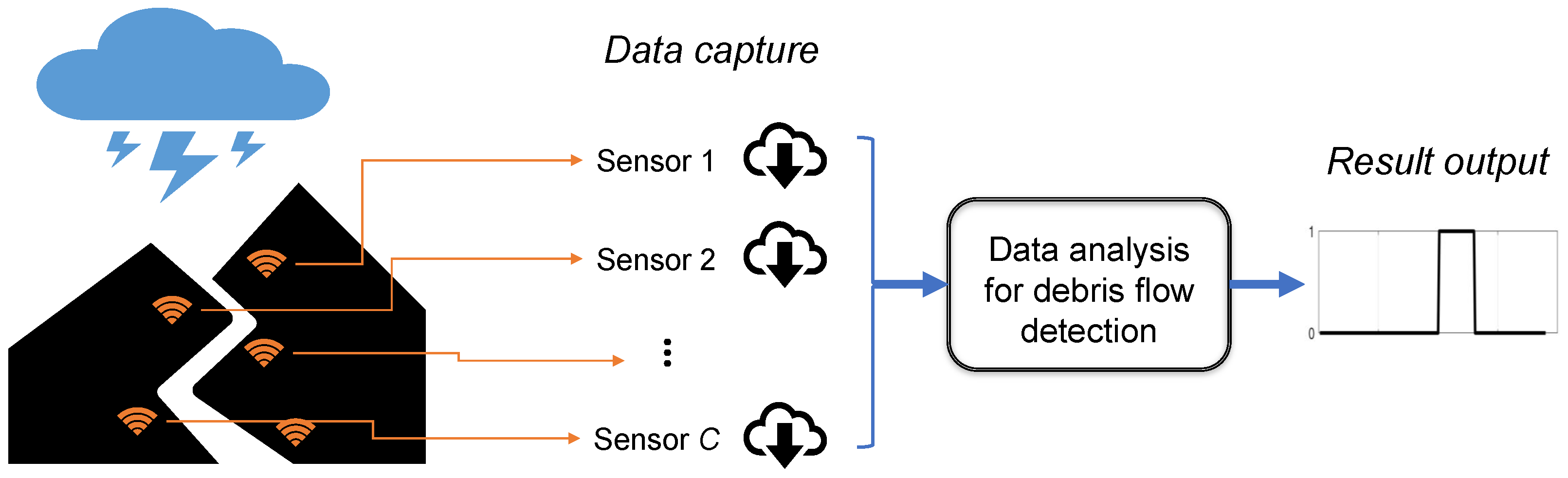
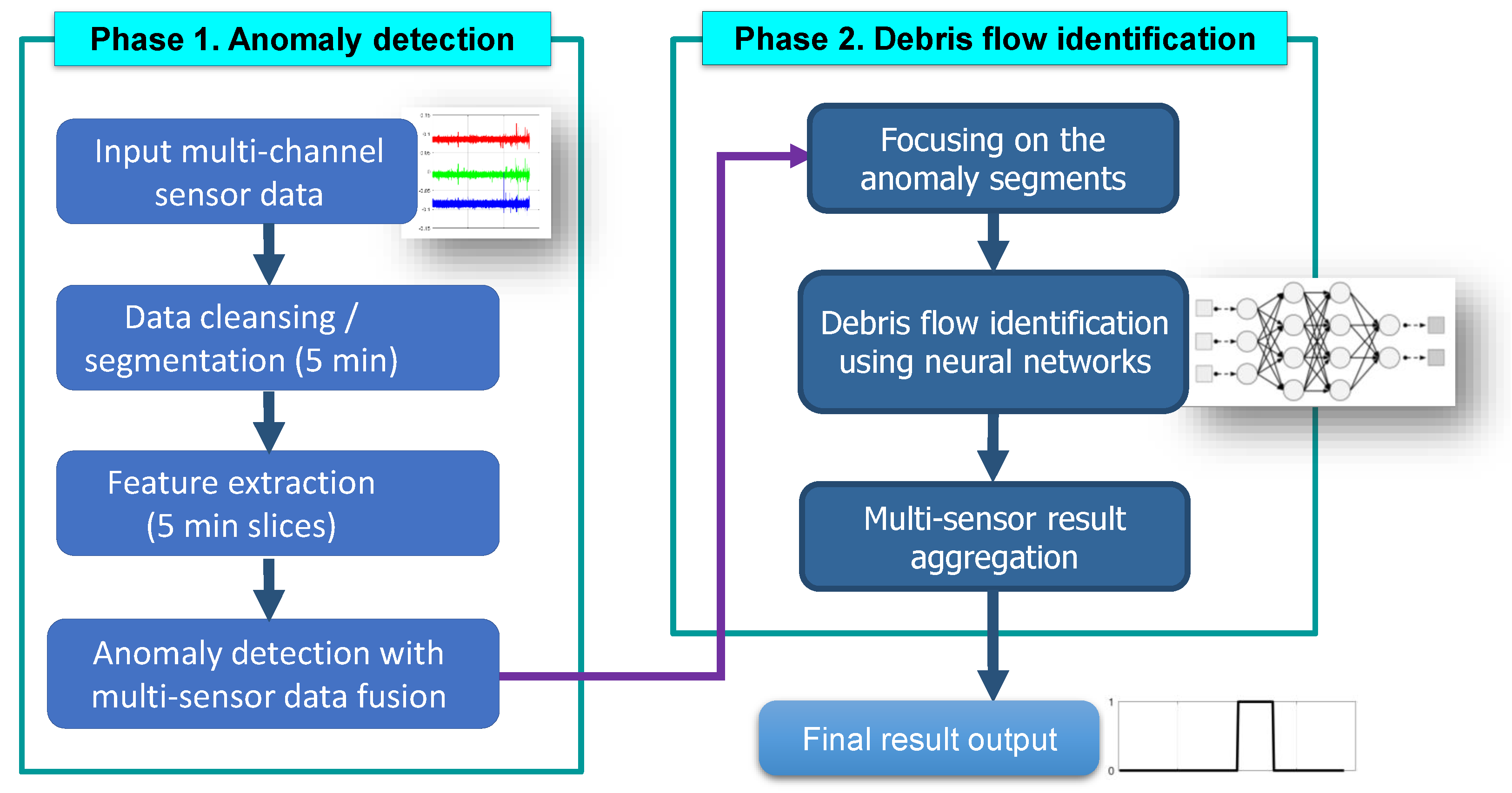
3.2. The Proposed Debris Flow Detection Algorithm

Within the context of debris flow monitoring, efficient content-level interpretation of input vibration data is the most critical step. Content/event retrieval from accelerometer data series had been a long-standing research theme in the field of signal processing and machine learning, such as in health care [21] and security fields [22]. We demonstrate the vibration data mining approach developed for debris flow monitoring in the following content.

Current accelerometer data investigation systems commonly have two major components: 1. Efficient feature extraction which converts the raw (dense) data to a compact form with discriminant information well retained to the task. 2. Statistical machine learning algorithms which are employed to perform content-based retrieval using extracted features. The latest advancement in machine learning techniques, which enables to characterize nonlinear relationships and interactions between multivariate data adequately, had been successfully adopted for modeling observations and measurements in various environmental fields such as hydrological forecasting [23] and satellite data processing [24]. In this study, we develop state-of-the-art machine learning algorithms to deal with multi-channel vibration data streams, and the overview diagram is presented in Figure 7. Concretely, first, we perform anomaly detection of the overall sensory data to get rid of a large volume of normal data that carry non-hazardous information in an unsupervised manner. Notably, there exists one major drawback in the first-round screening which cannot distinguish debris flow induced sensory data patterns from the ones generated by strong wind and heavy rain; and thus, we further devise a second-stage classification that identifies debris flow induced patterns among others. At this stage, we conducted an extensive comparative evaluation on a series of efficient machine learning algorithms, including logistic regression, support vector machine (SVM) [25] and deep neural networks [26], on real data and the results are exhibited in the validation section.

Before entering into the details of machine learning algorithm design, let us explain mathematical notions. The triaxial data gathered from c-th accelerometer sensor at t time frame is noted as ${\mathbf{s}}_t^c={[s^a,s^b,s^c]}_{t,c}^{\prime }$, where $a,b,c$ denotes the triaxial measurements, respectively. To characterize the continuous time-series data, we segment the data by using sliding windows with T data points. The resultant i-th clip can be expressed as ${\mathbf{x}}_i^c=[{\mathbf{s}}_1^c,{\mathbf{s}}_2^c,\dots ,{\mathbf{s}}_T^c]$ for the sake of brevity. Meanwhile, we perform error checking on sensor data to eliminate sensor faults. The resultant data clips are fed to the above-mentioned two-stage data investigation process for debris flow event identification.

3.2.1. Feature Extraction from Accelerometer Data

Feature representation plays a critical role in event-based accelerometer data interpretation, i.e., discerning debris flow-induced patterns, among others. As shown in Figure 6, different environmental stimuli, such as rain and debris flow, induce specific signal patterns, and feature extraction methods are employed to characterize the signal by using statistics and probabilities. Concretely, the primary purpose of accelerometer feature extraction is to find a set of characteristics such as, stationary property, entropy as a measure of uncertainty, summary statistical attributes of an interquartile range, which can adequately capture discriminant information presented in the observation window. Based on previous studies of accelerometer data mining [27], we established a vibration data feature library dedicated to the debris flow identification task.

Table 1. Feature list for accelerometer data characterization.

Accelerometer Features for Debris Flow Monitoring
Feature Type	Feature Name	Description
Time domain	1. Root mean square (RMS)	$RM{S}^c=\sqrt{\frac{1}{T}\sum {\mathbf{s}}_{t,c}^2},t\in [1,T]$
	2. Mean absolute deviation (MAD)	$MA{D}^c=\frac{1}{T}{\sum }_1^T{\mathbf{s}}_{t,c}-{\mu }_c,{\mu }_c=\frac{1}{T}\sum {\mathbf{s}}_{t,c}$
	3. Interquartile range (IQR)	Descriptive statistics as the difference between 75th and 25th percentiles
	4. Tilt of the sensor	$til{t}_c^1=\frac{1}{T}\sum |s_t^a|+|s_t^b|$
		$til{t}_c^2=\frac{1}{T}\sum |s_t^a|+|s_t^c|$
		$til{t}_c^3=\frac{1}{T}\sum |s_t^b|+|s_t^c|$
	5. Tilt ratio (TR) of the sensor	$T{R}_c^1=til{t}_c^1/\left|s_t^c\right|$
		$T{R}_c^2=til{t}_c^2/\left|s_t^b\right|$
		$T{R}_c^3=til{t}_c^3/\left|s_t^a\right|$
	6. Magnitude area (MA)	$M{A}_c=\frac{1}{T}\sum |{\mathbf{s}}_t^a|+|{\mathbf{s}}_t^b|+|{\mathbf{s}}_t^c|$
	7. Motion intensity (MI)	$M{I}_c=\frac{1}{T-1}{\sum }_{t=1}^{T-1}|{\mathbf{s}}_{t+1}^c-{\mathbf{s}}_t^c|$
	8. Maxima/Minima (M2M)	M2M =$\max \left({\mathbf{s}}_{t,c}^2\right)/\min \left({\mathbf{s}}_{t,c}^2\right),t\in [1,T]$
	9. Binned distribution (BD)	For input data, first calculate the range (R) as maximum–minimium; then, R is divided into 15 equal size bins which records the fraction of data values falls in.
	10. Zero cross rate (ZCR)	Zero-crossing count of the waveform
	11. Cross-axes correlation (CC)	Calculated for each pair of axes as the ratio of the covariance and the product of the standard deviations.
	12. Descriptive statistics	entropy, skewness and kurtosis
Spectral domain	13. Average band power (ABP)	Compute time-average of spectrogram of data
	14. Band standard deviation (BSD)	Compute standard deviation of each band along within observation window

demonstrates the detail list of the features and we extract 12 types of time domain features from triaxial data waveforms. Moreover, to exploit the physical displacement patterns of the sensor, we examine the cross-relational effects of different motion axes, i.e., taking cross-correlation of binary combinations of a-, b-, and c- into account as features. Time–frequency analysis is another efficient method to accelerometer pattern analysis [28], which is preferable to get rid of noises stay at a specific band. In this study, we extracted two types of spectral features for vibration data analysis. As a result, given one segmented data clip noted as ${\mathbf{x}}_i^c$, we obtain a series of characteristic features through the methods shown in Table 1. Then, we concatenate all feature values as the vector. In this study, the extracted feature is denoted as ${\mathbf{f}}_i^c$ where c is an index of sensor channel, and i represents ordinal number along time, respectively.

3.2.2. Data Analysis Phase 1: Anomaly Detection

In general, debris flow monitoring is to find a particular event of interest that sparsely superimposed in the continuous observation context. From this aspect, the monitoring data is anticipated to be highly redundant since the majority renders no hazardous information at all. To eliminate the data irrelevant to disaster monitoring with high efficiency and low computation cost, we employ the subspace method that is favorable for various anomaly detection tasks [29].

Subspace method characterizes the highest variance of a multi-dimensional dataset by using a lower dimensional linear subspace defined by a set of orthogonal eigenvectors. According to Figure 6, the normal data that contains no environmental stimuli commonly exhibit stationary characteristic, which can be effectively modeled by a subspace. On the contrary, heavy rain and debris flow can lead to a higher variability signal that may not reside in the subspace. Anomaly detection can be carried out by investigating deviation from input signal to the predominant pattern subspace. That is, the first k principal components returned by eigendecomposition of the data covariance matrix are used to form a “predominant pattern subspace,” since it captures the major patterns of normal data. During anomaly detection, all normal data tends to have almost zero length projection on the normal subspace. On the other hand, abnormal data induced by environmental impacts will exhibit significant deviations. We introduce the computational procedure as follows, and it begins with the computing correlation matrix of the input feature series ${\mathbf{F}}^c=[{\mathbf{f}}_1^c,\dots ,{\mathbf{f}}_n^c,\dots ,{\mathbf{f}}_N^c]$:

$$C_{\mathbf{D}}=\frac{1}{N}\sum _{n=1}^N{\mathbf{f}}_n{\mathbf{f}}_n^{\top },$$

(1)

then, eigen decomposition is performed:

$$\lambda \mathbf{v}=C_{\mathbf{D}}\mathbf{v}.$$

(2)

Let $\mathbf{P}=[{\mathbf{v}}_1,\dots ,{\mathbf{v}}_{K^{\prime }}]$ denotes subspace accommodating predominant textures, which is composed of $K^{\prime }$-th eigen vectors with highest eigenvalues. $K^{\prime }$ is determined by contribution rate which is defined as ${\eta }_K^{\prime }={\sum }_{k=1}^{K^{\prime }}{\lambda }_k/{\sum }_{k=1}^K{\lambda }_k$. Given input feature vector ${\mathbf{f}}_{\mathbf{in}}$ The deviation distance to subspace can be computed by:

$$h_{in}={{\mathbf{f}}_{\mathbf{in}}}^{\top }{\mathbf{f}}_{\mathbf{in}}-{{\mathbf{f}}_{\mathbf{in}}}^{\top }\mathbf{P}{\mathbf{P}}^{\top }{\mathbf{f}}_{\mathbf{in}}.$$

(3)

By examining the deviation distance $h_{in}$, we are able to detect outliers in the accelerometer data. Concretely, normal data, due to stationary characteristic, will generate quite low $h_{in}$. In contrast, intense vibrations aroused by environmental impacts will introduce distinct $h_{in}$ values; therefore, $h_{in}$ can be treated as an anomalous score indicating some event may happen regarded to monitoring area. By performing simple thresholding with a defined threshold $\tau$ and a gating function $g(·)$, we can convert continuous series of $h_{in}$ to discrete indexes, where 0 and 1 indicate normal and abnormal, respectively:

$$g\left(h_{in}\right)=\left\{\begin{array}{cc}1& h_{in}\ge \tau \\ 0& \mathrm{otherwise}\end{array}\right.$$

(4)

Above processing can be performed on each channel of sensor measurements, and then we further integrate individual judgment to produce overall output. The fusion rule is straightforward here that we employ logical AND overall channel’s anomaly detection results. In other words, we adopt a hypothesis that debris flow would generate significant displacements to all monitoring sensors installed along banks of the dam; and we had validated such assumption on real data. As a result, the anomaly detection algorithm screens out a large portion of non-hazardous data.

However, one significant issue remained in the current result, that is, by using subspace method, both debris flow and other extreme weather conditions such as heavy rain and strong wind will lead to high $h_{in}$ values, and hence, a further distinction can not be made. To tackle debris flow identification problem, we devised a second-stage pattern analysis process.

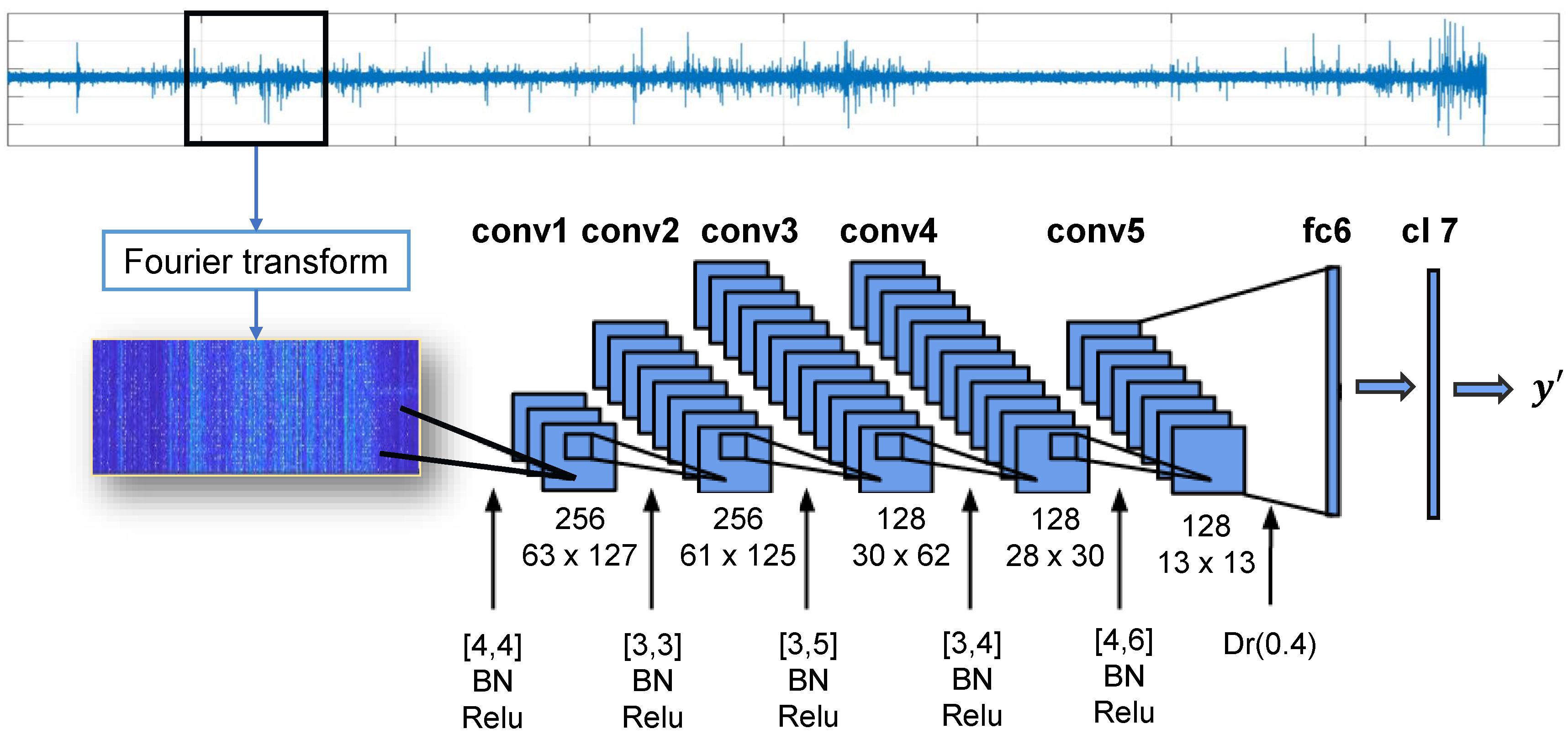
3.2.3. Data Analysis Phase 2: Debris Flow Identification

This section demonstrates the machine learning algorithm employed to discern the particular debris flow-induced signal patterns among others. Recently, deep neural networks have emerged as a series of learning models that are quite efficient to characterize complex/high-level abstractions from raw data [26]. The architecture is composed of multiple layers which perform the nonlinear transformation on the outputs of previous ones so that a hierarchy of computation interprets input data from low-level raw data values to high-level concepts. Deep learning models had achieved remarkable results in computer vision, and speech recognition [30], it has also been exploited for accelerometer data investigation under the context of human activity recognition [31]. In this study, we introduce deep convolution neural networks (CNN) to investigate the accelerometer signal for debris flow identification, by which convolution operators are designated to deal with two-dimensional data, such as vibration data spectrogram (time-frequency distribution) shown in Figure 6. Moreover, Figure 8 shows detail architecture of the proposed learning model which is composed of 5 convolution layers (conv1 ∼ conv5), one full connected layer (fc6) and a classification layer (cl7). First, we denote the computation model of deep neural networks as function $H(·)$, which encodes hierarchical structures. The mechanism of information propagation between layers, e.g., from $k-1$ layer to k, complies with the same principle that performs convolution operation to obtain a convolved feature map. The process can be expressed as follows:

$${\mathbf{h}}^{\left(k\right)}=g({\mathbf{b}}^{\left(k\right)}+{\mathbf{W}}^{\left(k\right)}{\mathbf{h}}^{(k-1)})$$

(5)

It is noteworthy that the $g(·)$, named as activation function, plays a critical role. We employ Rectified linear unit (ReLU), defined by $g(\rho ,a(k\left)\right)=\max (0,a(k\left)\right)+a\left(k\right)min(0,\rho )$, owing to two facts: 1. the embedded linear transform can effectively tackle gradient vanishing problem during model updates. 2. The formula encourages sparse activations, which can further suppress overfitting. Batch normalization (BN) is another efficient trick to facilitate deep learning and thus is adopted as a standard process. Furthermore, to avoid the model overfits to training data, at a full connected layer (fc6), we perform dropout on 40% weight of the whole deep model. Other key hyperparameters, such as convolution kernel size, resultant feature map size, and the number of filter banks are also presented in Figure 8.

The neural network training scheme is a vital issue throughout learning system development. We present a general training algorithm pseudo code in Algorithm 1 where $\frac{\partial L}{\partial \theta }$ is the derivative induced by the loss of training data, $ϵ$ is called the learning rate that governs the network update step/speed. From the diagram, we can see the prediction error is iteratively minimized by performing stochastic optimization, and we apply Adaptive Moment Estimation (ADAM) [30] due to the high processing efficiency and low memory usage. It is noteworthy that the data collection is assumed to highly imbalanced that usual observations greatly exceed the number of samples data with debris flow presence. In such scenario, classification rule that predicts the small classes tend to be rare, undiscovered or ignored; consequently, test samples belonging to the small classes, i.e., debris flow-induced patterns, are misclassified more often than those belonging to the prevalent classes. To deal with this issue, we employ penalized classification that imposes an extra cost on the model for making classification mistakes on the minority class (debris flow) during training [32]. The penalization weights for three classes of normal, rain or wind, and debris flow are set to [0.1, 0.2, 0.7], and it will guide the model to make fewer mistakes on debris flow classification throughout the training. In a practical scenario, the pre-trained deep learning system extracts critical information regarding disaster occurrence from the spectrogram of vibration data and then computes the probability of debris flow presence by using softmax function (cl7 layer). Furthermore, to validate the proposed approach, we performed the extensive experimental comparison between the proposed approach with various conventional machine learning algorithms, including Logistic regression (LR), regularized discriminant analysis (RDA) and support vector machine (SVM) [29].

Algorithm 1 Neural Network Training with back propagation

1: procedure Train Neural Net(${\mathbf{M}}_t,y_t,{\mathbf{W}}_t$)            ▹ t=0 2:   $\mathrm{Initialization}:\mathbf{W},\theta$ 3:   for $t=1,2,\dots ,T$ do 4:     $\mathrm{Perform}\mathrm{forward}\mathrm{propagation}:{\widehat{\mathit{y}}}_{\mathit{t}}=\mathit{H}({\mathbf{M}}_t,{\mathbf{W}}_H\left(\theta \right))$ 5:     $\mathrm{Compute}\mathrm{the}\mathrm{class}-\mathrm{wise}\mathrm{penalized}\mathrm{prediction}\mathrm{loss}:\mathit{L}({\mathit{y}}_{\mathit{t}},{\widehat{\mathit{y}}}_{\mathit{t}})$ 6:     $\mathrm{Update}\mathrm{weights}\mathrm{via}\mathrm{back}\mathrm{propagation}:{\theta }^t\leftarrow {\theta }^{t-1}-ϵ\frac{\partial L}{\partial \theta }$ 7:   return ${\mathbf{W}}_{\mathbf{H}}\left({\theta }_t\right)$

3.2.4. Efficient Sensor Fusion Scheme

Aiming at incorporating multi-channel sensory information for better debris flow monitoring, we adopt an effective computational scheme to exploit varying (relative) contribution concerning the sensor deployment locations. Fundamentally, the idea stems from the fact such as a sensor installed at a higher place is more susceptible to wind noise compare to the ones stay at lower regions; and thus it could be preferable to perform weighted averaging compared to arithmetic averaging. Precisely, we firstly define fusion rule through convex combination as follows:

$$y_{FUSION}=\frac{1}{C}\sum _1^C{\alpha }_c\times y_c,0\le {\alpha }_c\le 1,$$

(6)

where $y_c$ denote the judgment score estimated at c-th channel data. ${\alpha }_c$ is the contribution weight with respect to its location (indexed by c). The parameter of ${\alpha }_c$ can be inferred at validation stage during model training by using linear programming optimizer:

$$\underset{c}{arg\; min}\frac{1}{N}\sum _{n=1}^N{(y_n-(\frac{1}{C}\sum _1^C{\alpha }_c\times y_c))}^2,\sum _{c=1}^C{\alpha }_c=1.$$

(7)

4. Results

4.1. Data Collection and System Settings

To validate the proposed system for debris flow monitoring, we collected accelerometer data from the 3 June to the 4 July 2017. Onsite rain gauge and anemometer had been used to monitor weather condition. Besides, we applied wire sensors together with a surveillance camera to generate ground truth annotations for debris flow occurrence. Wire sensors can detect the time of debris flow strikes according to the level of the highest wire that has been broken by the flow. In Figure 9, we present three snapshots of monitoring camera showing wire sensor utility. Then, upon an investigation of both wire sensor output (time stamps of wire cut) and video clips, we collect the begin/end time annotations of debris flow occurrence, which are presented in

Table 2. Details of debris flow occurrence.

Case	Start Time	End Time2
1	7 Jun 2017 16:21:00	7 Jun 2017 17:00:00
2	20 Jun 2017 16:35:00	20 Jun 2017 18:05:00
3	24 Jun 2017 19:03:01	24 Jun 2017 20:05:00

.

Subsequently, we show the parameter settings of the proposed monitoring system. The sampling frequency of accelerometer data was set to 50 Hz, and streaming data analysis window length is fixed to 5-min. At the anomaly detection stage, the contribution rate ${\eta }_K^{\prime }$ is set as 0.99 to construct the normal vibration pattern subspace. To produce spectrogram of vibration data clips, we set the Fourier analysis window length to 1024 with 3/4 overlapping. To classify the input spectrogram of accelerometer data, we employ a deep convolution neural network (CNN) demonstrated in Section 4.3. During model training, we set the initial learning rate and mini-batch size as 1.0 × 10${}^{-3}$ and 96, respectively. To avoid overfitting, we employ L2 regularization with the regularization parameter set to 0.01; and the maximum updating epoch was set to 40. Besides, as suggested in many previous studies, the momentum parameter is set to 0.9 in stochastic gradient descent optimizer. At the evaluation stage, we performed a particular case of cross-validation called Leave-one-debris flow-out (LODO) scheme. Concretely, at each validation iteration, only one time of debris flow data is used for testing; while the model is trained on all the other debris data collections. As iteration goes, all the debris flow-induced vibration data can be tested. As a result, we obtain the predicted labels to the whole dataset.

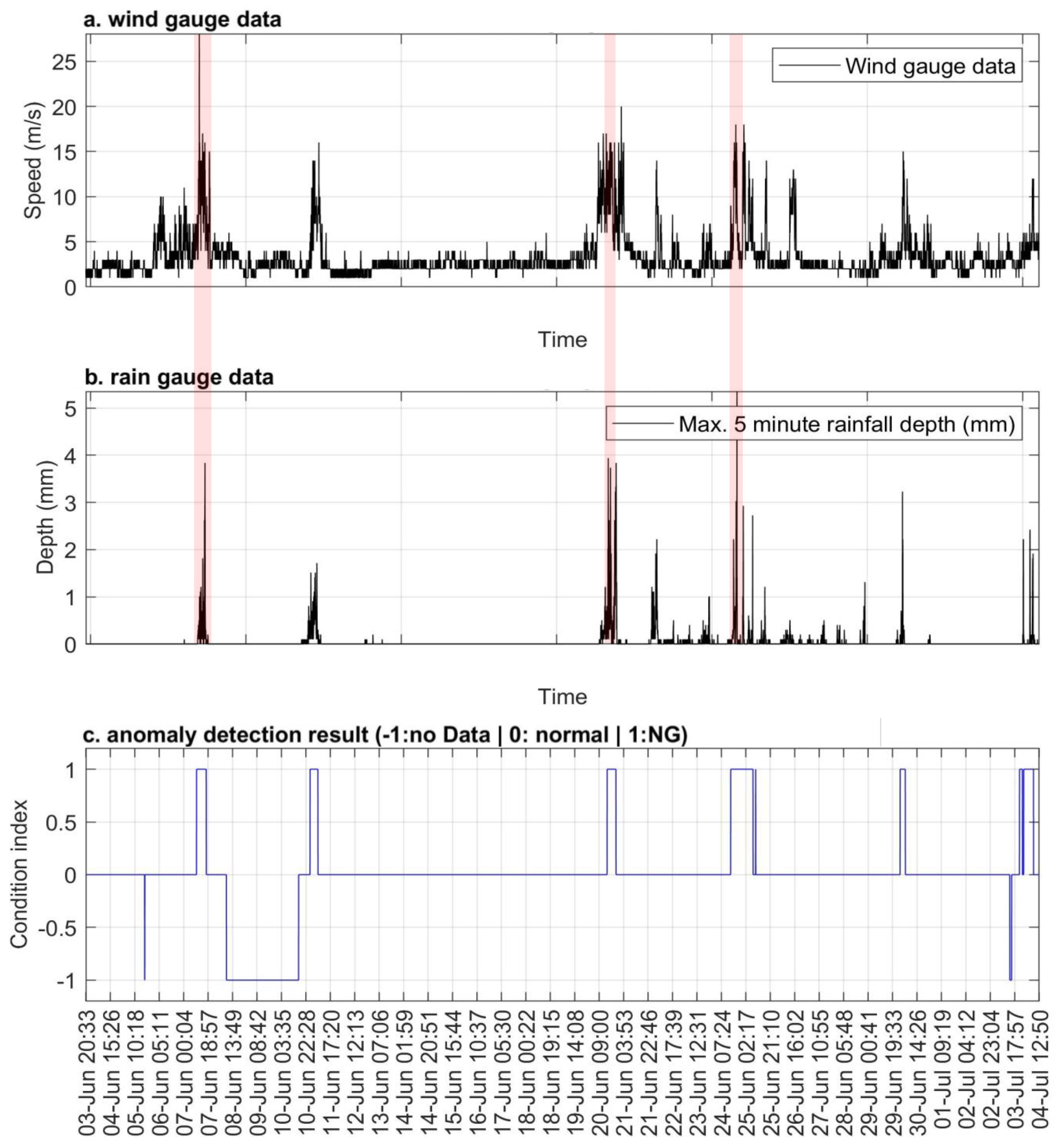
4.2. Anomaly Detection Result

This section covers the anomaly detection results for debris flow monitoring. We first present the wind and rain gauge data collected from 3 June to 4 July in Figure 10a,b, respectively. Those climate observations are essential because rainfall event had been deemed to be a significant factor that triggers a debris flow at Sakurajima [5]. Moreover, during the period three debris flow occurred, which were highlighted with pink color. By examining the data, we can see that heavy rain and strong winds often hit together; furthermore, we find that rain falls are necessary for inducing a debris flow, but not sufficient, such as in the case on 10 June. Such fact suggests that rain/wind gauge data cannot provide adequate information for debris flow prediction. Figure 10c shows the anomaly detection result generated by the algorithms demonstrated in Section 3. The whole dataset includes 8835 clips with 5-min length. According to the detection result, 619 segments are marked as suspicious of debris flow occurrence. As a result, the proposed anomaly detection scheme achieved a favorable 93% redundant data reduction without missing any debris flow occurrence. It is noteworthy that there existed much of false alarms which are resort to hostile weather conditions. To suppress such issue, we carry out further content-based classification with machine learning.

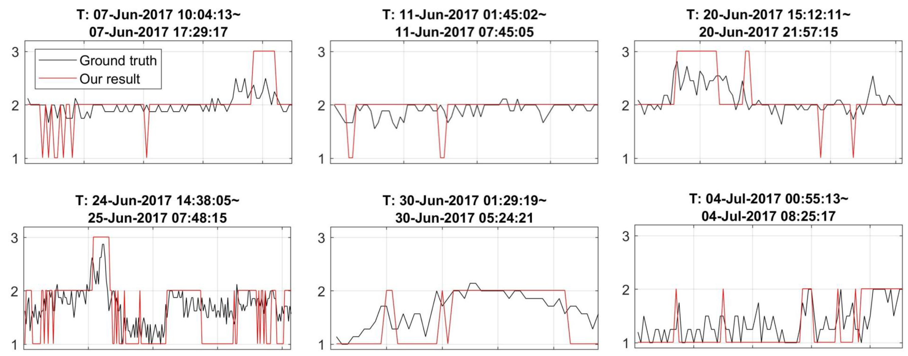
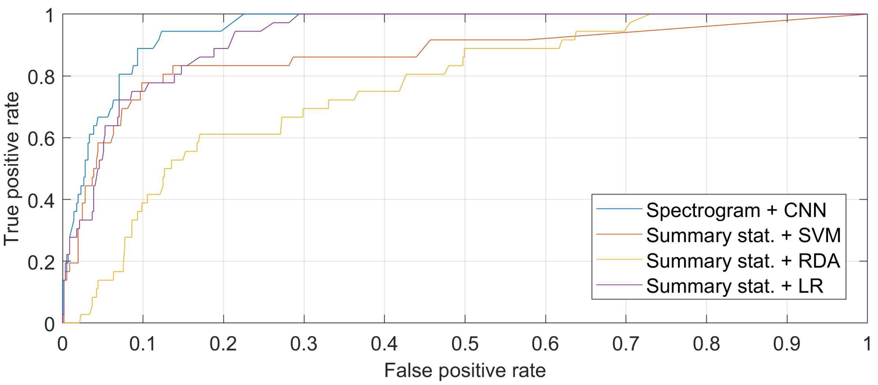
4.3. Debris Flow Identification Performance

Aiming at achieving high precision debris flow-induced vibration data pattern recognition, we conducted an extensive experimental comparison between conventional statistical classifiers and the devised deep learning model. It is noteworthy that those supervised algorithms require both data set and corresponded data labels. To this end, we investigated surveillance video data and assigned 3-valued class labels, in which label 1, 2 and 3 represent regular pattern, raining/wind, and debris flow occurrence on each 5 min data clip, respectively. We applied the convolution neural network demonstrated in Section 3.2.3 to assess the data membership belonging to the three categories. Subsequently, multi-accelerometer score fusion is applied, as explained in Section 3.2.4. We present the prediction results (fusion score) and data annotations on all 619 data clips in Figure 11. It is evident that debris flows can be discerned with a higher fusion scores ranging from 2 to 3. In contrast, non-hazardous data will get fusion scores lower than 2. Upon such observation, we further set the threshold to 2 on fusion score series for debris identification with binary outputs.

Moreover, to demonstrate the effectiveness of our approach, we conducted extensive comparison studies by using various feature/classifier combinations for the task. Precisely, in addition to adopting spectrogram of accelerometer data classification by using convolution neural networks, we evaluated the conventional approach by using various summary statistical features shown in Table 1 together with three primary conventional machine learning classifiers, including Logistic regression (LR), regularized discriminant analysis (RDA) and support vector machine (SVM). As for result comparison, receiver operating characteristic (ROC) curve was employed to demonstrate both false alarm and miss detection issues, simultaneously. Figure 12 illustrates all the results under comparison, where $\mathit{summary}\mathit{stat}.$ indicates using the conventional features shown in Table 1. The comparison results clarify that using accelerometer spectrogram with CNN model outperformed all other methods with a significant margin, and thus the effectiveness of the proposed approach had been validated.

5. Discussion

This study demonstrated that automatic debris flow detection could be achieved by using low-cost wireless accelerometer networks with an advanced machine learning algorithm. According to experimental validations, the proposed approach achieved favorable detection performance; that is, all the three debris flows can be successfully detected. Besides, we investigated the processing efficiency since the provision of timely and effective debris flow progress information are crucial to avoid or reduce the damages. Through evaluation, we confirmed that the developed wireless sensor networks are able to collect vibration data and transmit the data to local analysis workstation in real time even under extreme weather conditions. Subsequently, our debris flow detection algorithm is used to examine the multichannel vibration data clips with a fixed length of 5 min. In other words, the system can take at maximum of 5 min to analyze the latest data while recording the following streaming data. We evaluated the proposed algorithm by using a desktop PC with i9-7900K CPU with 128 GB memory and a laptop PC with i7-7500U CPU with 24 GB memory. Both hardware specifications can complete the data analysis process within a minute. In other words, the system can run for in-situ early detection of debris flow in a near real-time manner. Besides, with the increase of massive accelerometer data collection, the data-driven machine learning algorithm, such as deep convolution networks, is anticipated to achieve superior detection precision. Moreover, in our plan, we also expect to expand the current system by adding a new type of sensors for high precision and robust debris flow monitoring.

6. Conclusions

The main objective of this work was to design a computerized debris flow detection system, which consists of wireless accelerometer network hardware and machine learning algorithms to detect debris flows with high accuracy in real time. The proposed system renders a batch of favorable features for debris flow monitoring as follows. First, we devised an efficient wireless triaxial displacement sensor with a self-contained electrical power supply. The sensor is favorably low-cost and thus, allows us to perform (dense) sensor net-based debris flow detection. Secondly, monitoring data is anticipated to be highly redundant since extreme events such as debris flow rarely occur. To get rid of non-hazardous data efficiently, we extracted a list of statistical features from the massive accelerometer signal, and then, performed anomaly detection by using the subspace method. Third, we adopted the latest deep learning scheme to process accelerometer data for precise debris flow identification among other interferences, including strong wind and heavy rain. Furthermore, we integrated all individual sensor’s judgment to achieve more accurate and reliable debris flow detection. Experimental results on real data demonstrated the effectiveness of the proposed debris flow monitoring approach. Besides, the developed data pattern investigation framework can be generalized to deal with multi-modal sensory data, such as audio data and geophone signals; and we plan to expand the sensing data source to enhance the monitoring performance further.

References

1. Coussot, P.; Meunier, M. Recognition, classification and mechanical description of debris flows. Earth Sci. Rev. 1996, 40, 209–227. [Google Scholar] [CrossRef]
2. Hungr, O.; Evans, S.G.; Hutchinson, I.N. A Review of the Classification of Landslides of the Flow Type. Environ. Eng. Geosci. 2001, 7, 221–238. [Google Scholar] [CrossRef]
3. Takahashi, T. A review of Japanese debris flow research. Int. J. Eros. Control Eng. 2009, 2, 1–4. [Google Scholar] [CrossRef]
4. Landslide Disaster Cases in Recent Years. Available online: http://www.mlit.go.jp/mizukokudo/sabo/jirei.html (accessed on 15 August 2018).
5. Takeshi, T. Evolution of debris-flow monitoring methods on Sakurajima. Int. J. Erosion Control Eng. 2011, 4, 21–31. [Google Scholar] [CrossRef]
6. Marra, F.; Destro, E.; Nikolopoulos, E.I.; Zoccatelli, D.; Creutin, J.D.; Guzzetti, F.; Borga, M. Impact of rainfall spatial aggregation on the identification of debris flow occurrence thresholds. Hydrol. Earth Syst. Sci. 2017, 21, 4525–4532. [Google Scholar] [CrossRef] [Green Version]
7. Lee, H.C.; Banerjee, A.; Fang, Y.M.; Lee, B.J.; King, C.T. Design of a Multifunctional Wireless Sensor for In-Situ Monitoring of Debris Flows. IEEE Trans. Instrum. Meas. 2010, 59, 2958–2967. [Google Scholar] [CrossRef]
8. Baum, R.L.; Godt, J.W. Early warning of rainfall-induced shallow landslides and debris flows in the USA. Landslides 2010, 7, 259–272. [Google Scholar] [CrossRef]
9. Huang, C.J.; Yin, H.Y.; Chen, C.Y.; Yeh, C.H.; Wang, C.L. Ground vibrations produced by rock motions and debris flows. J. Geophys. Res. Earth Surf. 2007, 112, F02014. [Google Scholar] [CrossRef]
10. Berti, M.; Genevois, R.; LaHusen, R.; Simoni, A.; Tecca, P.R. Debris flow monitoring in the Acquabona watershed on the Dolomites (Italian Alps). Phys. Chem. Earth Part B Hydrol. Oceans Atmos. 2000, 25, 707–715. [Google Scholar] [CrossRef]
11. Arattano, M.; Marchi, L. Systems and sensors for debris-flow monitoring and warning. Sensors 2008, 8, 2436–2452. [Google Scholar] [CrossRef]
12. De la Piedra, A.; Benitez-Capistros, F.; Dominguez, F.; Touhafi, A. Wireless sensor networks for environmental research: A survey on limitations and challenges. In Proceedings of the Eurocon 2013, Zagreb, Croatia, 1–4 July 2013; pp. 267–274. [Google Scholar]
13. Alamdar, F.; Kalantari, M.; Rajabifard, A. Towards multi-agency sensor information integration for disaster management. Comput. Environ. Urban Syst. 2016, 56, 68–85. [Google Scholar] [CrossRef]
14. Schimmel, A.; Hübl, J. Automatic detection of debris flows and debris floods based on a combination of infrasound and seismic signals. Landslides 2016, 13, 1181–1196. [Google Scholar] [CrossRef]
15. Erdaş, Ç.B.; Atasoy, I.; Açıcı, K.; Oğul, H. Integrating features for accelerometer-based activity recognition. Procedia Comput. Sci. 2016, 98, 522–527. [Google Scholar] [CrossRef]
16. Zheng, A.; Amanda, C. Feature Engineering for Machine Learning: Principles and Techniques for Data Scientists; O’Reilly Media, Inc.: Newton, MA, USA, 2018. [Google Scholar]
17. Wan, S.; Lei, T.C. A knowledge-based decision support system to analyze the debris-flow problems at Chen-Yu-Lan River, Taiwan. Knowl.-Based Syst. 2009, 22, 580–588. [Google Scholar] [CrossRef]
18. Kern, A.N.; Addison, P.; Oommen, T.; Salazar, S.E.; Coffman, R.A. Machine learning based predictive modeling of debris flow probability following wildfire in the intermountain Western United States. Math. Geosci. 2017, 49, 717–735. [Google Scholar] [CrossRef]
19. Dou, J.; Yamagishi, H.; Pourghasemi, H.R.; Yunus, A.P.; Song, X.; Xu, Y.; Zhu, Z. An integrated artificial neural network model for the landslide susceptibility assessment of Osado Island, Japan. Nat. Hazards 2015, 78, 1749–1776. [Google Scholar] [CrossRef]
20. Pham, B.T.; Pradhan, B.; Bui, D.T.; Prakash, I.; Dholakia, M.B. A comparative study of different machine learning methods for landslide susceptibility assessment: A case study of Uttarakhand area (India). Environ. Model. Softw. 2016, 84, 240–250. [Google Scholar] [CrossRef]
21. Amini, N.; Sarrafzadeh, M.; Vahdatpour, A.; Xu, W. Accelerometer-based on-body sensor localization for health and medical monitoring applications. Pervasive Mob. Comput. 2011, 7, 746–760. [Google Scholar] [CrossRef] [PubMed] [Green Version]
22. Lee, W.H.; Lee, R.B. Multi-sensor authentication to improve smartphone security. In Proceedings of the 2015 International Conference on Information Systems Security and Privacy (ICISSP), Angers, France, 9–11 February 2015. [Google Scholar]
23. Yaseen, Z.M.; Allawi, M.F.; Yousif, A.A.; Jaafar, O.; Hamzah, F.M.; El-Shafie, A. Non-tuned machine learning approach for hydrological time series forecasting. Neural Comput. Appl. 2016, 30, 1479–1491. [Google Scholar] [CrossRef]
24. Li, W.; Ni, L.; Li, Z.L.; Duan, S.B.; Wu, H. Evaluation of Machine Learning Algorithms in Spatial Downscaling of MODIS Land Surface Temperature. IEEE J. Sel. Top. Appl. Earth Obs. Remote Sens. 2019. [Google Scholar] [CrossRef]
25. Murphy, K.P. Machine Learning: A Probabilistic Perspective; MIT Press: Cambridge, MA, USA, 2012. [Google Scholar]
26. LeCun, Y.; Bengio, Y.; Hinton, G. Deep learning. Nature 2015, 521, 436. [Google Scholar] [CrossRef] [PubMed]
27. González, S.; Sedano, J.; Villar, J.R.; Corchado, E.; Herrero, Á.; Baruque, B. Features and models for human activity recognition. Neurocomputing 2015, 167, 52–60. [Google Scholar] [CrossRef] [Green Version]
28. Machado, I.P.; Gomes, A.L.; Gamboa, H.; Paixão, V.; Costa, R.M. Human activity data discovery from triaxial accelerometer sensor: Non-supervised learning sensitivity to feature extraction parametrization. Inf. Process. Manag. 2015, 51, 204–214. [Google Scholar] [CrossRef]
29. Bishop, C.M. Pattern Recognition and Machine Learning; Springer: Berlin, Germany, 2006. [Google Scholar]
30. Goodfellow, I.; Bengio, Y.; Courville, A. Deep Learning; MIT Press: Cambridge, MA, USA, 2016. [Google Scholar]
31. Nweke, H.F.; Teh, Y.W.; Al-Garadi, M.A.; Alo, U.R. Deep learning algorithms for human activity recognition using mobile and wearable sensor networks: State of the art and research challenges. Expert Syst. Appl. 2018, 105, 233–261. [Google Scholar] [CrossRef]
32. López, V.; Fernández, A.; Moreno-Torres, J.G.; Herrera, F. Analysis of preprocessing vs. cost-sensitive learning for imbalanced classification. Open problems on intrinsic data characteristics. Expert Syst. Appl. 2012, 39, 6585–6608. [Google Scholar] [CrossRef]
Figure 1. Overview diagram of in-situ debris flow monitoring system.
Remotesensing 11 01512 g001
Figure 2. The map of study area: the debris monitoring site at Nojiri river No.7 dam (left). Sakurajima island (middle). Location of Sakurajima in Japan (right).
Remotesensing 11 01512 g002
Figure 3. Snapshots of monitoring camera: before (left) and during (right) debris flow.
Remotesensing 11 01512 g003
Figure 4. Internal design (left) and exterior look (right) of accelerometer unit.
Remotesensing 11 01512 g004
Figure 5. The deployment map of monitoring sensors, in which accelerometer sensors are marked with white circles.
Remotesensing 11 01512 g005
Figure 6. Examples of sensory data with respect to different environmental stimuli. The leftmost column shows raw waveforms with red, green and blue indicating x-/y-/z-axis, respectively. Also spectrogram (time-frequency distribution) plots of triaxial data are presented from 2nd to 4th column.
Remotesensing 11 01512 g006
Figure 7. The proposed two-phase accelerometer monitoring data investigation framework.
Remotesensing 11 01512 g007
Figure 8. Flow chart of the deep convolution neural network applied for accelerometer data investigation.
Remotesensing 11 01512 g008
Figure 9. Snapshots of wire sensor utility. The conditions of before/during/after debris flow strikes are shown from left to right, respectively.
Remotesensing 11 01512 g009
Figure 10. Anomaly detection result for debris flow monitoring, confirming with environmental conditions.
Remotesensing 11 01512 g010
Figure 11. Validation of debris flow identification result, in which the scores above 2 indicate debris flow occurrence.
Remotesensing 11 01512 g011
Figure 12. Debris flow identification performance comparison between various data pattern classification methods.
Remotesensing 11 01512 g012