New Approach for Temporal Stability Evaluation of Pseudo-Invariant Calibration Sites (PICS)

Abstract

Pseudo-Invariant Calibration Sites (PICS) are one of the most popular methods for in-flight vicarious radiometric calibration of Earth remote sensing satellites. The fundamental question of PICS temporal stability has not been adequately addressed. However, the main purpose of this work is to evaluate the temporal stability of a few PICS using a new approach. The analysis was performed over six PICS (Libya 1, Libya 4, Niger 1, Niger 2, Egypt 1 and Sudan 1). The concept of a “Virtual Constellation” was developed to provide greater temporal coverage and also to overcome the dependence limitation of any specific characteristic derived from one particular sensor. TOA reflectance data from four sensors consistently demonstrating “stable” calibration to within 5%—the Landsat 7 ETM+ (Enhanced Thematic Mapper Plus), Landsat 8 OLI (Operational Land Imager), Terra MODIS (Moderate Resolution Imaging Spectroradiometer) and Sentinel-2A MSI (Multispectral Instrument)–were merged into a seamless dataset. Instead of using the traditional method of trend analysis (Student’s T test), a nonparametric Seasonal Mann-Kendall test was used for determining the PICS stability. The analysis results indicate that Libya 4 and Egypt 1 do not exhibit any monotonic trend in six reflective solar bands common to all of the studied sensors, indicating temporal stability. A decreasing monotonic trend was statistically detected in all bands, except SWIR 2, for Sudan 1 and the Green and Red bands for Niger 1. An increasing trend was detected in the Blue band for Niger 2 and the NIR band for Libya 1. These results do not suggest abandoning PICS as a viable calibration source. Rather, they indicate that PICS temporal stability cannot be assumed and should be regularly monitored as part of the sensor calibration process.

1. Introduction

Remote sensing using orbiting satellite sensors is essential for detecting and monitoring changes in the Earth’s land surfaces, oceans, atmosphere and climate [1]. The number of orbiting Earth Observation (EO) satellites has increased dramatically within the past decade. By 2017, over 150 EO satellites were launched, mostly “small” satellites operated by commercial vendors. One of the challenges emerging from the growing use of EO satellite sensors is achieving accurate radiometric calibration of individual sensors and establishing a baseline calibration among multiple sensors. Radiometric calibration is essential for the use of remote sensing data in quantitative applications such as climate change monitoring, ocean measurements, vegetation measurements and so forth. Regular in-flight calibration assesses the sensor’s on-orbit performance throughout its operating lifetime. These can be performed on data acquired from an on-board calibration source, such as a solar diffuser panel, and/or acquisition of radiance measurements from the Earth’s surface through vicarious calibration methods. It is important to highlight that a significant portion of the cost saving is achievable with small EO satellite sensors by removing on-board calibration source. For these sensors, vicarious calibration is the preferred option. Perhaps the three most commonly used vicarious calibration methods are: reflectance-based approach [2], cross-calibration [3]; and analysis of Pseudo-Invariant Calibration Sites (PICS) image data [4,5]. Performing in-situ vicarious calibration at many of these sites is not possible due to their geographic remoteness and/or political instability. Consequently, research is increasingly focused on vicarious calibration based on satellite sensor observations of selected PICS [6]. The current work focuses on the last method.

There has been a significant increase in the use of PICS over the last 14 years to monitor the long-term top-of atmosphere (TOA) reflectance trends from different sensors [4,7,8]. Govaerts et al., for example, have developed an operational calibration method using bright desert calibration sites to support geostationary satellite data [9,10]. In order to evaluate the in-flight calibration performance of optical satellite sensors, the selection of reference PICS based on certain criteria such as the site’s radiometric and spectral stability is a challenging task. Sites should be chosen such that a sufficient number of overpasses occur for as many sensors as possible so that they can be used in a sensor’s long-term performance monitoring [11]. In addition, there are some intrinsic properties for choosing PICS which typically include data availability, spatial uniformity, temporal stability and spectral uniformity [12]. Moreover, the site should be located in higher altitude arid or desert regions to minimize atmospheric effects. The Committee on Earth Observation Satellites (CEOS) has developed an online catalog of candidate test sites meeting these criteria [6]. Six of these sites have been officially designated as “reference” PICS appropriate for satellite sensor calibration and monitoring sensor radiometric performance [6]: Libya 1, Libya 4, Mauritania 1, Mauritania 2, Algeria 3 and Algeria 5.

Previous research has yielded significant advances in PICS-based on-orbit sensor calibration and monitoring of sensor radiometric performance. Morstad and Helder [13] developed an approach for the calibration of the Landsat 5 TM using images of the Sonoran Desert as a candidate PICS. Chander et al. [14] assessed the on-orbit calibration stability of the Terra MODIS and Landsat 7 ETM+ sensors based on analysis of Libya 4 image data; their results indicated a change in sensor-measured TOA reflectance of approximately 0.4% per year or less over a 10-year period.

The underlying assumption of the PICS-based calibration is that the site is “invariant” – or pseudo invariant, so any detected change in the lifetime trend is attributed solely to sensor response. However, is it valid to assume that the sites are invariant over time? Previously, by assuming site invariance, little emphasis was given to developing an explicit assessment of a site’s temporal stability. Therefore, the main objective of this work is to evaluate the temporal stability of PICS using a new approach. Stability of pseudo invariant sites should to be tested before their use in monitoring post-launch radiometric calibration stability of satellite sensors. Once a site’s temporal stability is assured, the analysis of sensor stability based on these invariant sites can be undertaken with greater confidence.

The key technique of this work involves the implementation of a process to “homogenize” TOA reflectance data from multiple sensors for a given PICS, creating a Virtual Constellation (VC) TOA reflectance dataset for that site. The VC is a recent concept developed by CEOS in support of the Group on Earth Observations (GEO) objectives and as the space component of the Global Earth Observation System of Systems (GEOSS). According to CEOS a VC is a “coordinated set of space and/or ground segment capabilities from different partners that focuses on observing a particular parameter or set of parameters of the Earth system” [15]. Claverie et al. [16], for example, used this new concept to describe sensor data homogenization of the Landsat 8 (L8) Operational Land Imager (OLI) and Sentinel 2A/Sentinel 2B (S2A/S2B) Multispectral Instrument (MSI) surface reflectance products. Such homogenization requires pre-processing before merging data from multiple sensors to create a smooth time series dataset. Helder et al. [17] provided valuable recommendations to achieve this based on observations relating to cross-calibration between the OLI and MSI sensors to achieve better data interoperability.

The primary goal of this work is to determine the temporal stability of six PICS commonly used in calibration analyses by the South Dakota State University Image Processing Laboratory (SDSU IPLAB): Niger 1, Niger 2, Libya 1, Libya 4, Egypt 1 and Sudan 1. The four sensors studied in this work are the Landsat 8 OLI, Landsat 7 ETM+, Terra MODIS and Sentinel 2A MSI. These sensors were selected for the following reasons: (i) previous research has consistently established their radiometric calibration to within 5% [18,19,20]; (ii) the local equatorial crossing times for these sensors are close, thus they can image a given region under similar solar illumination and atmospheric conditions; and iii) large amounts of data for these sensors are widely and freely available. It is shown that the individual sensor’s TOA reflectance datasets, in one or more bands, violate one or more conditions required for proper application of the Student’s T-test, which has traditionally been employed for drift analyses [14,18]. For the purposes of this work, the “appropriate” statistical analysis is non-parametric in nature. The data from these sensors for a particular PICS were combined into a single TOA reflectance dataset, with the intent of reducing the effects of discrepancies in sensor radiometric performance such as spectral response and solar/sensor viewing geometry. The stability assessment of the site was determined from the TOA reflectance temporal trend of the combined dataset. In principle, this work could be done using the TOA reflectance data from an individual sensor, under the assumption the sensor response is not degrading over time. However, the use of multiple sensors offers increased temporal resolution of the dataset and also overcomes the dependence limitation of any one particular sensor. Moreover, the span of data acquisition is not similar across all sensors. Therefore, direct comparison of the trends between individual sensors might yield different conclusions about a given site’s temporal stability (e.g., one sensor’s trend suggests the site is changing while another sensor’s trend suggests it is not). Finally, statistical analysis was performed on the VC to identify potential monotonic trends in the TOA reflectance.

2. Satellite Sensor Overview: Landsat-8 OLI, Landsat-7 ETM+, Sentinel-2A MSI and Terra MODIS

This section provides a brief overview of the sensors investigated for this work. The basic performance characteristics for each sensor are presented in

Table 1. Basic Sensor Characteristics [1,3,4,8,14,18].

Characteristics	Landsat 8-OLI	Landsat 7-ETM+	Sentinel 2A-MSI	Terra MODIS
Number of Bands	11	8	13	36
Spatial Resolution	30 m	15 m, 30 m, 60 m	10 m, 20 m, 60 m	250 m, 500 m, 1000 m
Swath Width	185 km	183 km	295 km	2330 km
Spectral Coverage	0.4–1.38 µm	0.4–14 µm	0.4–2.2 µm	0.4–12.5 µm
Pixel Quantization	12 bits	8 bits	12 bits	12 bits
Launch Date	11 February 2013	15 April 1999	23 June 2015	18 December 1999
Temporal Resolution	16 days	16 days	5 days	1–2 days
Orbit Type	Sun-synchronous	Sun-synchronous	Sun-synchronous	Sun-synchronous
Equatorial Crossing Time	10:13 a.m.	10:00 a.m.	10:30 a.m.	10:30 a.m.
Altitude	705 km	705 km	786 km	705 km

.

The Landsat series of sensors have acquired the longest continuous series of image observations of the Earth’s surface [19]. Prior to the launch of L8, the Landsat-7 Enhanced Thematic Mapper Plus (ETM+) was considered to be the most stable of the Landsat series, with estimated uncertainties in its at-sensor radiance calibration of ±5% [3]. Until very recently, the ETM+ has employed radiance based-calibration [21]. The ETM+ detector performance has been more stable than its on-board calibrators [22]. Angal et al. [21] showed in their cross-calibration work of ETM+ and MODIS that both instruments demonstrate high temporal stability in spectrally matching bands with 2% long term drifts for more than 18 years.

The OLI has been performing well, providing high quality data for Earth observation and the prelaunch calibration of the Landsat-8 OLI had an estimated uncertainty of approximately 3% in reflectance products. Subsequent post-launch reflectance-based calibrations have consistently demonstrated uncertainties on the order of 2% or less [23]. OLI radiometric calibration and stability are monitored by on-board calibrators and it was found that except for the Coastal/Aerosol band (CA), other bands are stable to within 0.3% [24].

The MODIS is a key instrument onboard the Terra and Aqua satellites operated as a part of NASA’s (National Aeronautics and Space Administration) Earth Observing System. MODIS data is used for a wide range of applications such as ocean, land, atmosphere and climate monitoring. It has operated successfully on-board for the last 19 years. For Terra MODIS TOA reflectance products, a calibration uncertainty of approximately ±2% has been estimated [3,25]. The MODIS instrument acquires data at three spatial resolutions—250 m, 500 m and 1 km, which are coarser than the other sensors used in the study. In contrast, MODIS presents the highest temporal resolution (near-daily revisit acquisition capability).

Sentinel-2A was the first in the Sentinel-2 series of satellites launched for the Copernicus program developed by the European Space Agency (ESA). The main purpose of this sensor is to provide stable image data of high spatial resolution (10 to 60 m) [26]. Time series data obtained from its onboard sensor, the Multi-Spectral Instrument (MSI), are comparable to OLI and other well calibrated sensor data [26]. Barsi et al. [27] demonstrated that OLI and MSI showed stable radiometric calibration, with consistency between matching spectral bands to approximately ~2.5%. According to the Sentinel-2 Mission Requirement Document, the instrument has stringent radiometric requirements: (a) the absolute radiometric uncertainty shall be better than 5% (the goal is 3%); (b) the inter-band relative radiometric uncertainty data shall be constant from one spectral band to any other one to better than 3% over the reduced dynamic range; (c) the requirement between the satellites (cross-satellite) is 3% [28].

In order to analyze the stability of pseudo-invariant sites using the Virtual Constellation approach, it is necessary for all sensors to image common ground targets in the same regions or spectral bands of the electromagnetic spectrum. For the sensors investigated in this work, the common bands are designated as “Blue,” “Green,” “Red,” “NIR,” “SWIR1” and “SWIR2.”

Table 2. Sensor Spectral Bands.

Bandwidth (nm)
Sensor	Blue	Green	Red	NIR	SWIR 1	SWIR 2
OLI	452–512 (b2)	533–590 (b3)	636–673 (b4)	851–879 (b5)	1567–1651 (b6)	2107–2294 (b7)
ETM+	441–514 (b1)	519–611 (b2)	631–692 (b3)	772–898 (b4)	1547–1748 (b5)	2064–2346 (b7)
MSI	470–524 (b2)	504–602 (b3)	649–680 (b4)	855–875 (b-8a)	1569–1658 (b11)	2113–2286 (b12)
MODIS	459–479 (b3)	545–564 (b4)	620–670 (b1)	841–876 (b2)	1628–1652 (b6)	2105–2155 (b7)

gives the corresponding wavelength ranges of each band for each sensor. The Relative Spectral Responses in analogous bands for these sensors are presented in Figure 1.

3. Study Area (PICS Sites)

Helder et al. [29] developed an automated invariant site identification algorithm to locate statistically optimal regions. The results from this work suggested that temporal stability in the range of 1–3% could be achieved by using the CEOS referenced sites. In another study, Mishra et al. [30] ranked the CEOS referenced test sites according to temporal uncertainty estimated from an analysis of ETM+ data. In this work, the six SDSU IPLAB PICS across North Africa were evaluated (Figure 2). The temporal uncertainties of these six PICS in each of the spectral bands from visible to shortwave infrared (SWIR) were found to be less than other CEOS-recommended PICS (e.g., Mauritania 1, Mauritania 2, Algeria 3, Algeria 5 and Mali) [30]. The center latitude and longitude coordinates for each site are given with the corresponding site name: (1) Libya 4 (28.55°N, 23.38°E); (2) Libya 1 (24.70°N, 13.49°E); (3) Niger 1 (9.36°N, 20.41°E); (4) Niger 2 (10.44°N, 21.08°E); (5) Sudan 1 (21.40°N, 27.70°E); and (6) Egypt 1 (27.41°N, 26.38°E). The Region of Interest (ROI) within each PICS have been chosen based on previous studies [31]. The algorithm was developed by the SDSU IPLAB, known as PICS normalization process (PNP), identified the regions within the PICS, which are specified as “Optimal Region.” This means that all pixels inside the selected ROIs in this work present at least 3% temporal, spatial and spectral variability. In other words, the selected ROI presents temporal, spatial and spectral stability equal or better than 3%. Figure 2 shows the optimal region for each site as the white pixels and the selected ROI for each site as a blue rectangle.

Table 3. WRS-2 Path/Row and Center ROI coordinates of selected PICS.

PICS	WRS-2 Path/Row	Minimum Latitude	Minimum Longitude	Maximum Latitude	Maximum Longitude	Center Latitude	Center Longitude
Libya 4	181/40	28.38	23.09	28.81	23.86	28.55° N	23.38° E
Libya 1	187/43	24.55	13.32	24.86	13.66	24.70° N	13.49° E
Niger 1	189/46	20.28	9.19	20.53	9.52	9.36° N	20.41° E
Niger 2	188/45	21.25	10.38	21.47	10.71	10.44° N	21.08° E
Sudan1	177/45	21.40	27.81	21.75	27.59	21.40° N	27.70° E
Egypt1	179/41	26.91	26.31	27.13	26.62	27.41° N	26.38° E

gives the corresponding corner latitude and longitude coordinates defining the ROI, along with the corresponding Landsat World-wide Reference System 2 (WRS2) path and row.

4. Methodology

Due to differences in sensor design, the radiometric responses for each sensor are not the same. As part of the data processing described in this section, these differences must be reduced such that all sensors measure a common radiance/reflectance level.

4.1. Image Pre-Processing

All of the Landsat ETM+ and OLI images used in this study were downloaded to the SDSU IPLAB archive from the United States Geological Survey (USGS) Earth Resources Observation and Science (EROS) Data Center (https://earthexplorer.usgs.gov/). Similarly, Sentinel 2 MSI images were retrieved from the Copernicus Open Access Hub (https://scihub.copernicus.eu/). All MODIS data products can be accessed from the Earth Data website (http://earthdata.nasa.gov/). Here, the MODIS Collection 6.1 was used, since it represents the best available MODIS data. Lyapustin et al. [32] describes the latest version of the algorithm used for processing the MODIS Collection 6 data record. Finally, the MODIS Characterization Support Team (MCST) provided the Terra MODIS imagery. All of the downloaded image products were pre-processed by each group to remove radiometric and geometric artifacts. The OLI, ETM+ and MSI products were then scaled to 16-bit integers representing TOA reflectance; the MODIS products were processed to produce TOA reflectance values [14]. Additional details describing the various pre-processing steps can be found on each group’s web site.

4.2. Conversion to TOA Reflectance

For the OLI, ETM+ and MSI, the pixel values for each ROI at each site were then converted to TOA reflectance using linear scaling factors given in the associated product metadata. For the ETM+ and OLI, the TOA reflectance is directly obtained as follows [33]:

$${\mathsf{\rho }}_{\mathsf{\lambda }}^{\prime }{= \mathrm{M}}_{\mathsf{\rho }}{\ast \mathrm{Q}}_{\mathrm{Cal} }{+\mathrm{A}}_{\mathsf{\rho }}$$

(1)

where ${\mathsf{\rho }}_{\mathsf{\lambda }}^{\prime }$ is the estimated TOA reflectance, ${\mathrm{Q}}_{\mathrm{Cal} }$ is the calibrated DN pixel value and ${ \mathrm{M}}_{\mathsf{\rho }}$ and ${\mathrm{A}}_{\mathsf{\rho }}$ are band-specific, reflectance-based multiplicative and additive scaling factors, respectively. These scaling factors were designed to account for the estimated exoatmospheric solar irradiance that is needed for radiance-to-reflectance conversion, which can vary according to the model (Chance-Kurutz (ChKur) solar spectrum) used to calculate it [34], as well as the seasonal variation in the Earth-Sun distance. However, these coefficients do not account for solar zenith angle (SZA), so an additional cosine correction is required:

$${\mathsf{\rho }}_{\mathsf{\lambda }}=\frac{{\mathsf{\rho }}_{\mathsf{\lambda }}^{\prime }}{\cos \left(\mathrm{SZA}\right)}$$

(2)

Conversion of MSI pixel values to TOA reflectance just involves scaling by a single constant which accounts for the exoatmospheric irradiance, Earth-sun distance and any required cosine correction:

$${\mathsf{\rho }}_{\mathsf{\lambda }}= \frac{{\mathrm{DN}}_{\mathrm{cal}}}{\mathrm{g}}$$

(3)

where ${\mathrm{DN}}_{\mathrm{cal}}$ is the 12-bit (calibrated DN) pixel value and $\mathrm{g}$ = 10000 is the currently established scale factor.

For MODIS, the reflectance information for the six PICS was received from the NASA MCST. Using the same region of interest as shown in Figure 2, the at-sensor reflectance values on a per-pixel basis were extracted for each MODIS band used in this study. These values were computed at the native spatial resolution of each MODIS band (250 m for bands 1, 2, 3 and 4 and 500 m for bands 6 and 7) and then averaged over the ROI. The Level 1B calibrated products used for this work are from Collection 6.1, the version reflecting the latest calibration algorithms from MCST. The irradiance model used by the MODIS instrument is basically the combination of different irradiance models [35,36,37].

4.3. Data Filtering

Once the mean TOA reflectance value for each image’s ROI was calculated, filtering was required to ensure only cloud-free image data were analyzed. ETM+ and OLI image data were filtered in part using the associated quality band information. In the case of MODIS, the MODIS cloud-mask product was used—which provides the information about cloud-presence at 1 km spatial resolution [38]. If over 50% of the pixels were flagged as “cloudy” for any scene, then it was excluded from the process. For all sensors, an empirical 2-sigma (2σ) filtering approach (i.e., 2 standard deviations from the mean of the temporal TOA reflectance derived from all scenes) was applied, as Median Absolute Deviation (MAD) and other mean-based approaches were found to be too “aggressive” in removing potential outliers. Any image’s mean TOA reflectance for the ROI exceeding the 2σ threshold resulted in visual inspection of the image for all spectral bands; if the visual inspection indicated clouds/shadows or other artifacts not identified in the quality data, the scene was excluded from further analysis. Note that when cloud/shadows were detected in the ROI for any spectral band of an image, the entire scene (all spectral bands) was discarded from the analysis.

4.4. Bidirectional Reflectance Distribution Function (BRDF) Correction

The TOA reflectance of a given target can vary significantly from one acquisition to the next depending on the solar and sensor positions at each acquisition time. This effect is modeled by the Bidirectional Reflectance Distribution Function (BRDF). BRDF effects can also occur due to variations in orientation between multiple sensors co-incidentally imaging the same target with the same solar position.

For this analysis, BRDF correction of the mean TOA reflectance data from each scene was based on a multilinear regression model derived from the solar zenith/azimuth and sensor zenith/azimuth angles. Additional details describing this multilinear BRDF correction can be found in Reference [39].

$${\mathsf{\rho }}_{\mathrm{model}}{= \mathsf{\beta }}_0{+\mathsf{\beta }}_1{\mathrm{Y}}_1{+\mathsf{\beta }}_2{\mathrm{X}}_1{+\mathsf{\beta }}_3{\mathrm{Y}}_2{+\mathsf{\beta }}_4{\mathrm{X}}_2$$

(4)

where ${\mathsf{\beta }}_0,$ ${\mathsf{\beta }}_1$, ${\mathsf{\beta }}_2$, ${\mathsf{\beta }}_3$, ${\mathsf{\beta }}_4$ are the model coefficients. Y₁, X₁, Y₂ and X₂ are Cartesian coordinates representing the planar projections of the solar and sensor angles originally given in spherical coordinates:

$${\mathrm{Y}}_1=\sin \left(\mathrm{SZA}\right)\ast \sin \left(\mathrm{SAA}\right)$$

(5)

$${\mathrm{X}}_1=\sin \left(\mathrm{SZA}\right)\ast \cos \left(\mathrm{SAA}\right)$$

(6)

$${\mathrm{Y}}_2=\sin \left(\mathrm{VZA}\right)\ast \sin \left(\mathrm{VAA}\right)$$

(7)

$${\mathrm{X}}_2=\sin \left(\mathrm{VZA}\right)\ast \cos \left(\mathrm{VAA}\right)$$

(8)

where SZA, SAA, VZA and VAA are the solar zenith, solar azimuth, view zenith and view azimuth angles, respectively. The BRDF-corrected TOA reflectance for each sensor was determined as follows:

$${\mathsf{\rho }}_{\mathrm{BRDF}-\mathrm{corrected}} = \frac{{\mathsf{\rho }}_{\mathrm{obs}}}{{\mathsf{\rho }}_{\mathrm{model}}}{\times \mathsf{\rho }}_{\mathrm{ref}}$$

(9)

Here, ${\mathsf{\rho }}_{\mathrm{obs}}$ is the observed mean TOA reflectance from each scene. ${\mathsf{\rho }}_{\mathrm{model}}$ is the model predicted TOA reflectance. ${ \mathsf{\rho }}_{\mathrm{ref}}$ is the TOA reflectance with respect to a set of “reference” solar and sensor position angles; for this analysis, the reference SZA, SAA, VZA and VAA angles were calculated as the mean of the corresponding SZA, SAA, VZA and VAA angles from all processed scenes.

It is important to highlight that the MODIS Field of View (FOV) is approximately ±49.5°. However, in this work only at nadir or near-nadir viewing images were used. The variation in the view zenith angles for different PICS is less than 10 degrees. The scenes with larger view angles have not been included in the analysis. In addition, for the Sentinel and Landsat instruments the effect of angular variations within the ROI may not be negligible. Both instruments have a per-pixel solar zenith angle variation product. For the purposes of this work, BRDF correction was performed using the angular information for the pixels within the selected ROI (and not the scene-center angle information).

4.5. Scaling Adjustment

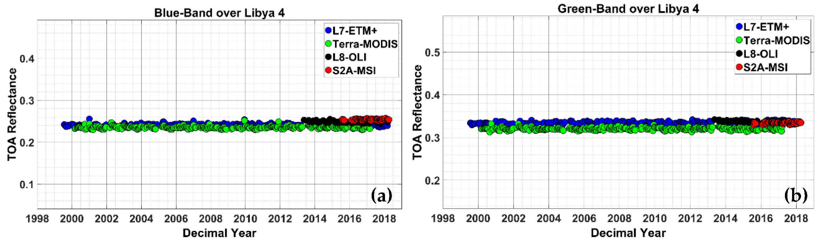
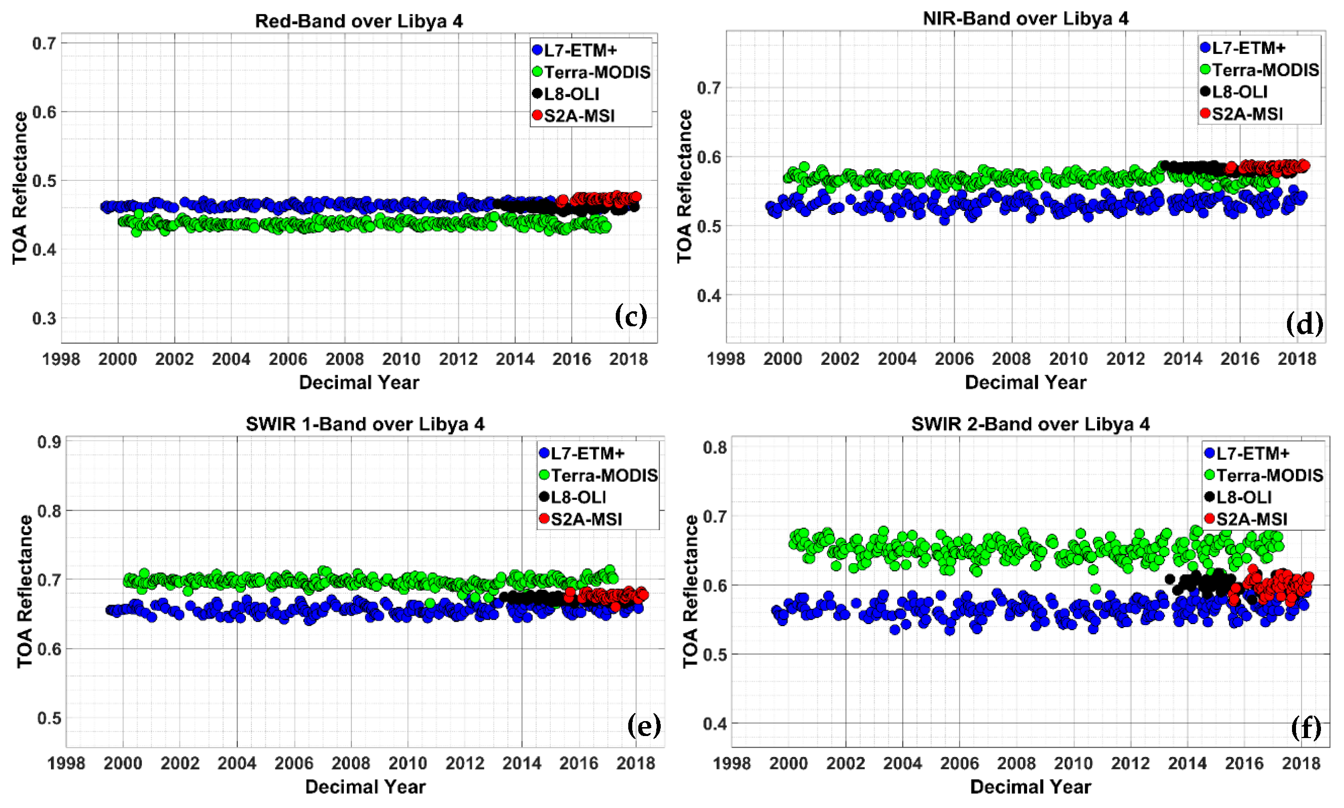
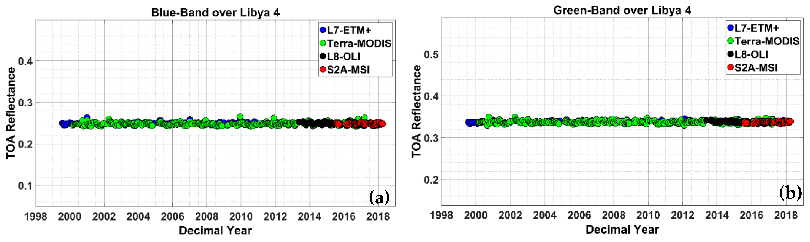
PICS site stability was initially evaluated based on analyses of an individual sensor’s BRDF-corrected TOA reflectance trend. As will be shown in Section 5, this initial approach produced contradictory conclusions among the sensors, primarily due to significant differences in their operating lifetimes affecting the amount of available data (e.g., the Sentinel-2A MSI has actively acquired image data for only three years, while the Landsat-7 ETM+ has actively acquired image data for almost 20 years). To provide a “common” operating lifetime, the BRDF-corrected mean TOA reflectance datasets for all sensors were pooled to produce a single time series dataset. The responses of the ETM+, MODIS and MSI were scaled by an adjustment factor to match the observed OLI response. For each sensor, the required adjustment factor was calculated as the mean of the ratios of the BRDF-corrected mean TOA reflectance values from near-coincident acquisitions with the OLI.

“Near-coincident acquisitions” refer to the scenes which are imaged within a maximum acceptable window of days; as for MODIS and OLI, “near-coincident” refers to the scene pairs imaged approximately 8 days apart. Finally, the TOA reflectance of each sensor was then normalized by the adjustment factor. It should be stated here that the proposed scaling adjustment can account for all types of differences (including the RSR differences) between the OLI and other sensors. Therefore, the SBAF normalization using Hyperion was not performed here.

4.6. Linearity Check for Individual Sites

Once the BRDF-corrected mean TOA reflectance datasets were generated for each sensor at each site, linear regressions were performed to characterize the temporal responses:

$${\mathsf{\rho }}_{\mathrm{i}}{= \mathsf{\alpha }}_1{\mathrm{t}}_{\mathrm{i} }{+ \mathsf{\alpha }}_0$$

(10)

where ${\mathrm{t}}_{\mathrm{i} }$ is the decimal year, ${\mathsf{\rho }}_{\mathrm{i}}$ is the BRDF-corrected mean TOA reflectance for a test site for a given sensor, ${ \mathsf{\alpha }}_1$ is the slope of the regression line and ${\mathsf{\alpha }}_0$ is the associated intercept. To determine whether a linear relationship between mean TOA reflectance and decimal year could be identified, a correlation test was performed for each site for each individual sensor.

Table 4. Correlation between Decimal Year and BRDF Corrected Mean TOA Reflectance of Libya 4.

	L8-OLI		L7-ETM+		S2A-MSI		Terra MODIS
Bands	Pvalue	Correlation	Pvalue	Correlation	Pvalue	Correlation	Pvalue	Correlation
Blue	0.0046	Yes	0.035	Yes	0.509	No	0.128	No
Green	0.0012	Yes	0.190	No	0.052	No	0.695	No
Red	0.0252	Yes	0.005	Yes	0.014	Yes	0.194	No
NIR	0.0004	Yes	0.003	Yes	0.192	No	0.342	No
SWIR1	0.0150	Yes	0.069	No	0.322	No	0.213	No
SWIR2	0.5118	No	0.009	Yes	0.111	No	0.656	No

and

Table 5. Correlation between Decimal Year and BRDF Corrected band adjusted combined Mean TOA Reflectance of Libya 4.

Virtual Constellation (OLI, ETM+, MSI and MODIS)
Bands	P Value	Correlation
Blue	0.4848	No
Green	0.4467	No
Red	0.0104	Yes
NIR	0.0130	Yes
SWIR 1	0.1949	No
SWIR 2	0.1595	No

present the correlation test results for Libya 4 for individual sensors and for the virtual constellation, respectively. In summary, there was sufficient statistical evidence to indicate a linear relationship between BRDF-corrected mean TOA reflectance and decimal year only for the OLI and ETM+ in most bands. For the MSI there was insufficient evidence to indicate a linear relationship in most bands and for MODIS, there was insufficient evidence in any band. Correlation tests performed for the other sites also exhibited inconsistencies in identification of a linear relationship across all bands. Based on these results, application of any statistical test expecting a linear relationship between BRDF-corrected mean TOA reflectance and time would likely lead to potentially misleading conclusions. It is possible that higher-order polynomial or even nonlinear relationships are present in the data.

4.7. Normality Check for Individual Sites

Mendes and Pala (2003) [40], studied the power of three normality tests. According to the authors Shapiro-Wilk was the most powerful test regardless of distribution and sample size and they recommend it to be used when testing for normality. In addition, in a more recent study, Yap and Sim (2011) [41], compared the power of eight normality test based on Monte Carlo simulation. According to their study, the results show that Shapiro–Wilk test is a powerful test regardless of distribution (symmetric short-tailed, symmetric long-tailed or asymmetric distributions). That is why this test was performed to determine whether the BRDF-corrected mean TOA reflectance values for each sensor and site represent samples obtained from a normally distributed population. Figure 3a,b, respectively, show the histograms of ETM+ Blue and SWIR2 band TOA reflectance obtained for Libya 4. Visual inspection of these histograms shows the appearance of a right-skewed tail in the Blue band histogram and a slight left-skewed tail in the SWIR2 band histogram, suggesting a non-normal distribution. This hypothesis is confirmed with the Shapiro-Wilk test results for all ETM+ bands from Libya 4, indicating the data are not normally distributed. The MODIS and MSI test results indicate their data are not normally distributed in some bands for this site. Interestingly, the OLI test results indicate its data are normally distributed in all bands. The particular Shapiro-Wilk results for each band using the Libya 4 data are summarized in

Table 6. Shapiro-Wilk Normality Test of BRDF-corrected Mean TOA Reflectance of Libya 4 by Sensor, α = 0.05.

Band	L8-OLI	L7-ETM+	S2A-MSI	Terra MODIS	Combined Sensor
Blue	Normal	Non-normal	Normal	Non-normal	Non-normal
Green	Normal	Non-normal	Normal	Non-normal	Non-normal
Red	Normal	Non-normal	Normal	Normal	Normal
NIR	Normal	Normal	Normal	Normal	Non-normal
SWIR 1	Normal	Normal	Non-normal	Non-normal	Non-normal
SWIR 2	Normal	Normal	Normal	Normal	Normal

.

The Shapiro-Wilk normality test result for combined sensor data also shows non-normal (Table 6) distribution of TOA reflectance for 4 bands whereas for the remaining two bands normal distribution is indicated. Application of the Shapiro-Wilk test to the reflectance data from the other sites suggests non-normality of reflectance data in at least some of the bands for all the sensors. Based on these results, application of any statistical test expecting normally distributed BRDF-corrected mean TOA reflectance values could likely result in to potentially misleading conclusions.

4.8. Statistical Tests for Trend Analysis

As mentioned previously, the Student’s T-Test has traditionally been used to evaluate satellite sensor performance based on PICS data analysis. Chander et al. [14] used linear regression as well as the T-Test to evaluate long term sensor stability of the ETM+ and MODIS. Angal et al. [42] used the T-Test to evaluate long term drift of TOA Reflectance over CEOS reference test sites for ETM+ and MODIS Collections 5 and 6. However, as shown in Section 4.6 and Section 4.7, the linearity and normality assumptions for the T-test do not apply to all bands in the individual and combined TOA reflectance datasets. Nonparametric statistical tests, such as the Mann-Kendall test, do not require assumptions of linearity and/or normality in the dataset. Thus, this test was selected for detection of potential monotonic trends.

4.8.1. Mann-Kendall Trend Test

The Mann-Kendall test is a widely used non-parametric test for identification of trends in a time series dataset [43,44,45]. The test has been extended to account for seasonal variation within the dataset, leading to its use in analyses of environmental and climatological data [43]. The Mann-Kendall test evaluates whether a series of values tend to increase or decrease over time through what is essentially a nonparametric form of monotonic trend regression analysis. This test analyzes the sign of the difference between later-measured data and earlier-measured data (see Equation (11)). For the purposes of this analysis, the seasonal Mann-Kendall test was performed at the 0.05 significance level on the hypotheses:

H1. 

no monotonic trend/Observations are random.

H2. 

monotonic trend, with the direction of trend dependent on the sign of the Mann-Kendall statistic,${\mathrm{S}}_{\mathrm{k}}$, for each season$\mathrm{k}$, calculated from the temporally sorted dataset:

$${\mathrm{S}}_{\mathrm{k}}= {\displaystyle \sum }_{\mathrm{i} = 1}^{{\mathrm{n}}_{\mathrm{k}}-1}{\displaystyle \sum }_{\mathrm{j} = \mathrm{i} +1}^{{\mathrm{n}}_{\mathrm{k}}}{\mathrm{sgn}(\mathrm{Y}}_{\mathrm{jk}}{-\mathrm{Y}}_{\mathrm{ik}})$$

(11)

where${\mathrm{Y}}_{\mathrm{jk}}$and${\mathrm{Y}}_{\mathrm{ik}}$are observations from season k in years j and i, respectively and${\mathrm{n}}_{\mathrm{k}}$is the number of years including season k. The sign of certain argument$\mathrm{X}$is defined as follows:

$$\mathrm{sgn} \left(\mathrm{X}\right) = \{\begin{array}{c} 1 \mathrm{if} \mathrm{X} > 0\\ 0 \mathrm{if} \mathrm{X} = 0\\ -1 \mathrm{if} \mathrm{X} < 0\end{array}$$

(12)

These statistics are summed up for the $\mathrm{p}$ different seasons to estimate the overall test statistic ${\mathrm{S}}_{\mathrm{n}}$:

$${ \mathrm{S}}_{\mathrm{n}} ={\displaystyle \sum }_{\mathrm{k} = 1}^{\mathrm{p}}{\mathrm{S}}_{\mathrm{k}}$$

(13)

If ${\mathrm{S}}_{\mathrm{n}}$ is positive, later values tend to be larger than earlier values and an upward trend is indicated. If S_n is negative, later values tend to be smaller than earlier values and a downward trend is indicated. If the p-value for S_n is less than the empirical significance level (0.05), there is sufficient evidence to reject the null hypothesis and conclude that there is a monotonic trend. Otherwise, there is insufficient evidence to conclude that a monotonic trend exists. It has already been stated that the sensors in this study are well calibrated with some degree of uncertainties, so if a monotonic trend (upward or downward) is found, it indicates changes to the site’s stability.

In any kind of hypothesis testing, the choice of decision making is a challenging task. Therefore, the concept of “Type I” and “Type II” errors should be mentioned here. “Type I” error arises for rejecting null hypothesis when it is actually true, also known as a “False Positive.” In other words, this error is because of accepting alternative hypothesis. Type I error is generally reported as the p-value. Usually, the common practice is to set Type I error as 0.05 or 0.01—this means there is 5 or 1 in 100 chance that the trend that we are observing is because of chance. This is called “Level of Significance.” Significance level needs to be chosen very carefully for getting rid of “Type I” error.

“Type II” error arises for not rejecting null hypothesis when the alternative hypothesis is true. In case of trend analysis, “Type II” error occurs when we fail to observe the presence of a monotonic trend when the truth is the presence of a monotonic trend.

4.8.2. Chi-Square Test

In this work one more statistical test was also performed, the Chi-Square test. This test is used to determine if there is significant difference between the expected and observed values. The value of the Chi-Square statistic indicates the disagreement between the observed values and the values expected under a statistical model, including any uncertainties. The test has the following statistic:

$${\mathrm{X}}^2= {\displaystyle \sum }\frac{{{(\mathrm{y}}_{\mathrm{i}}{-\mathrm{f}(\mathrm{x}}_{\mathrm{i}}\left)\right)}^2}{{\mathsf{\sigma }}^2}$$

(14)

where y_i is the measurement of the quantity y, when the quantity x is ${\mathrm{x}}_{\mathrm{i}}$; $\mathrm{f}\left({\mathrm{x}}_{\mathrm{i}}\right)$ is the expected value obtained from the linear models and ${\mathsf{\sigma }}^2$ is the uncertainty of y_i. In the analysis, chi-square test statistics have been calculated for two linear models for the mean TOA reflectance—one model includes the slope ($\mathrm{y} = \mathrm{mx} + \mathrm{c}$), while the other model is based on the mean TOA reflectance ($\mathrm{y} = \mathrm{c}$). Thereafter, the chi-square test statistics were compared from these two models to see whether they matched with the monotonic trend analysis results. This similarity/dissimilarity of results would indicate the effect of all types of calculation uncertainty in the trend analysis.

5. Results and Discussion

In the following sections, trend analysis results are shown for the Libya 4 site exclusively. This is because Libya 4 has been extensively used for sensor performance determination for a long time [5,14]. For the remaining PICS, a summary of the results is included thereafter.

5.1. Individual Sensor Trend Analysis

Figure 4 shows the long-term TOA reflectance trends over the Libya 4 PICS for spectrally matching bands of ETM+, OLI, MODIS and S2A MSI. The trends shown here have been BRDF corrected to minimize effects due to seasonal behavior. The normalization is effective in the visible and NIR bands; residual seasonality is apparent in NIR and both SWIR bands, particularly in SWIR 2. The trends for the ETM+, OLI and MSI overlap in the visible bands and are offset slightly in the NIR and SWIR bands. However, the MODIS reflectance is lower in the visible bands and significantly higher in the SWIR bands, with larger offsets occurring at the longer wavelengths. These offsets are caused by several factors, including the spectral signature of the ground target, differences due to the RSR (as described in Section 2) and atmospheric effects. In the NIR band, the MODIS and ETM+ reflectance trends are offset from the OLI and MSI trends.

To evaluate the long-term stability of the four sensors, the non-parametric Seasonal Mann-Kendall test was applied to the individual sensor datasets, according to the hypotheses stated in Section 4.8.2.

Table 7. Seasonal Mann-Kendall Test Results by Sensor for Libya 4 PICS, Significance level α = 0.05.

Band	Kendall Correlation Coefficient	S Statistic Value	P Value	Decision
Landsat -7 ETM+
Blue	−0.066	−71	0.2691	No Trend
Green	0.086	93	0.1466	No Trend
Red	0.151	163	0.0106	Upward Trend
NIR	0.269	289	0.0000	Upward Trend
SWIR 1	0.278	299	0.0000	Upward Trend
SWIR 2	0.213	229	0.0003	Upward Trend
TERRA MODIS
Blue	0.088	111	0.1211	No Trend
Green	0.072	91	0.2046	No Trend
Red	0.089	113	0.1146	No Trend
NIR	0.076	97	0.1761	No Trend
SWIR 1	−0.063	−80	0.2656	No Trend
SWIR 2	−0.004	−5	0.9551	No Trend
Landsat-8 OLI
Blue	−0.254	−15	0.1319	No Trend
Green	−0.424	−25	0.009	Downward Trend
Red	−0.373	−22	0.023	Downward Trend
NIR	−0.39	−23	0.0166	Downward Trend
SWIR 1	−0.458	−27	0.0051	Downward Trend
SWIR 2	−0.085	−5	0.6668	No Trend
Sentinel-2A MSI
Blue	0.150	3	0.6721	No Trend
Green	0.500	10	0.0624	No Trend
Red	0.300	6	0.3006	No Trend
NIR	0.300	6	0.3006	No Trend
SWIR 1	0.350	7	0.2042	No Trend
SWIR 2	−0.200	−4	0.5346	No Trend

Note: Kendall correlation coefficient is a nonparametric measure of the strength and association that exists between two variables measured on at least an ordinal scale. It returns a value between 0 and 1; 0 value of it refers to no relationship and 1 refers to a perfect relationship.

shows the analysis results. For the given significance level (0.05), there is insufficient evidence to indicate a monotonic trend in any band of the MODIS and MSI TOA reflectance datasets; for the ETM+ and OLI datasets, there is sufficient evidence to indicate monotonic trends are present in some of the bands. In this case, the individual sensor results are contradictory with respect to potential change in the site; no definite conclusion can be drawn. In addition, the potential trends identified in the ETM+ and OLI datasets appear to be in opposite directions for some of the analogous bands. Again, no definite conclusions regarding site stability can (or should) be drawn based on these results. To overcome this limitation, the TOA reflectance virtual constellation approach using multiples satellite Sensors is presented in the next section.

The Kendall correlation coefficient is also a good indicator for the presence of trend in any dataset. From Table 7, it can be stated that where the S statistic value is higher, the Kendall correlation coefficient is also higher. This coefficient provides consistency with the S statistic value to indicate trend.

5.1.1. Libya 4 PICS Stability Analysis

To address the ambiguous result described in the previous section, a data homogenization technique was applied to create a “combined” TOA reflectance dataset (Virtual Constellation). The technique consisted of applying a sensor-specific Scaling Adjustment factor to the TOA reflectance datasets, as described in Section 4.5. Figure 5a–f show the resulting trends for all sensors in each band. In comparison to the non-adjusted datasets shown in Figure 4a–f, there is excellent agreement between each sensor’s TOA reflectance values (even though seasonality effects are still observable in the SWIR bands). As a result, a seamless TOA reflectance dataset was created. As mentioned in Section 4.5, this Scaling Adjustment can account for additional sources of disagreement between sensors, including RSR differences.

Table 8. Scaling Adjustment Factors for Libya 4 PICS for each Sensor, by Band (Normalized to OLI).

Band	L7- ETM+	Terra-MODIS	S2A-MSI
Blue	1.015	0.980	1.021
Green	1.010	1.027	1.005
Red	1.004	1.028	0.994
NIR	0.992	1.004	0.996
SWIR 1	1.004	0.994	0.995
SWIR 2	1.002	1.001	1.005

includes the estimated Scaling Adjustment factors for each of the 3 sensors (ETM+, MODIS and MSI) over Libya 4 site to normalize the TOA reflectance to OLI’s TOA reflectance.

Table 9. Mean Percentage difference of mean TOA reflectance of L8 and the other 3 sensors before and after Scaling Adjustment normalization over Libya 4 site.

Sensor	L7- ETM+		Terra-MODIS		S2A-MSI
Bands	Before	After	Before	After	Before	After
Blue	−3.13	−0.07	−5.39	−0.27	2.06	0.06
Green	−0.98	0.13	−5.03	0.01	−1.07	0.03
Red	0.78	0.18	−5.10	−0.11	2.76	0.02
NIR	−8.62	0.35	−2.38	−0.06	0.45	0.02
SWIR 1	−2.16	0.33	3.65	0.10	0.67	0.01
SWIR 2	−5.86	0.40	8.34	−0.16	−0.35	0.04

shows the disagreement in mean TOA reflectance between the OLI and the other sensors before and after scaling adjustment normalization. The maximum disagreement between the OLI and S2A-MSI is consistently less than 3% before normalization and less than 0.1% after normalization; this is mainly due to mismatches in their RSRs. Disagreement between the OLI and MODIS significantly decreased, from over 8% before normalization to less than 0.3% after normalization. Similarly, disagreement between the OLI and ETM+ decreased from over 8.6% before normalization to approximately 0.4% after normalization. Clearly, the Scaling Adjustment has significantly reduced effects due to all differences in sensor response, including differences in relative spectral response and perhaps accounting for atmospheric effects as well. The increased agreement should allow for a more definitive analysis of site stability.

Figure 6 shows the combined TOA reflectance datasets over Libya 4 for corresponding bands in all sensors. The Seasonal Mann-Kendall test was applied to the combined dataset at the same significance level as that used for the tests on the individual sensor data.

Table 10. Seasonal Mann Kendall test result of Trend Analysis of Libya 4 (homogenized TOA reflectance data).

Band	Kendall Correlation Coefficient	S Statistic Value	P-Value	Decision
Blue	0.072	120	0.1507	No Trend
Green	0.098	162	0.0979	No Trend
Red	0.119	197	0.1408	No Trend
NIR	0.131	217	0.0862	No Trend
SWIR 1	–0.063	−105	0.3717	No Trend
SWIR 2	0.077	127	0.2878	No Trend

shows the results from this test. For the given significance level and estimated p-values, there is insufficient statistical evidence to indicate the presence of a long-term monotonic trend in TOA reflectance for any band of the combined dataset. However, the presence of short-term trends cannot be ruled out.

This section presented the results of a stability analysis of the combined Libya 4 dataset. The next sections present the results of similar analyses conducted at the remaining PICS studied in this work.

5.1.2. Virtual Constellation Trend Analysis

The concept of virtual constellation has already been introduced in the previous sections.

Table 11. Total number of scenes used for each site in trend analysis.

Sites	Libya 4	Egypt 1	Niger 1	Niger 2	Sudan 1	Libya 1
Number of homogenized Scenes	642	769	702	727	732	712

shows the number of datasets available after pre-processing for combining TOA reflectance data from 4 different sensors. It is clear that the number of combined/homogenized scenes of each PICS is sufficiently large enough for temporal analysis to detect small changes in time series datasets of PICS.

5.1.3. Egypt 1, Sudan 1, Niger 1, Niger 2 and Libya 1 Stability Analysis

Figure 7 shows the BRDF-corrected band adjusted homogenized mean TOA reflectance trend for the Egypt 1, Sudan 1, Niger 1, Niger 2 and Libya 1. As with Libya 4, seasonal variability and sensor response differences are significantly accounted for with the BRDF and Scaling Adjustment normalizations. At Libya 1, however, there appears to be potential outliers in TOA reflectance, particularly in the longer wavelength bands. These potential outliers should not be cloud-related, as pixels in the ROIs were visually checked and excluded from analysis if obvious clouds and/or cloud shadows were identified. Even though they appear as potential outliers, they were not excluded for the trend analysis, as all TOA reflectance data from each scene represent valid measurements used for trend detection.

Table 12. Seasonal Mann-Kendall test results for Combined Sensor TOA Reflectance Datasets at Remaining SDSU Sites, α = 0.05.

Band	Kendall Correlation Coefficient	S-Statistic Value	P-Value	Decision
Egypt 1
Blue	0.088	176	0.1285	No Trend
Green	0.082	164	0.2659	No Trend
Red	0.098	196	0.1880	No Trend
NIR	0.144	287	0.0616	No Trend
SWIR 1	0.051	102	0.6014	No Trend
SWIR 2	0.161	321	0.0510	No Trend
Sudan 1
Blue	–0.195	–365	0.0500	Downward Trend
Green	–0.275	–516	0.0040	Downward Trend
Red	–0.193	–362	0.0178	Downward Trend
NIR	–0.175	–328	0.0210	Downward Trend
SWIR 1	–0.259	–485	0.0033	Downward Trend
SWIR 2	–0.006	–11	0.9058	No Trend
Niger 2
Blue	0.207	377	0.0002	Upward Trend
Green	0.055	100	0.2744	No Trend
Red	0.079	145	0.1444	No Trend
NIR	0.071	130	0.2498	No Trend
SWIR 1	–0.090	–164	0.3031	No Trend
SWIR 2	0.035	63	0.6517	No Trend
Niger 1
Blue	0.078	145	0.1286	No Trend
Green	–0.147	–272	0.0191	Downward Trend
Red	–0.164	–305	0.0080	Downward Trend
NIR	–0.120	–222	0.0624	No Trend
SWIR 1	–0.129	–240	0.0533	No Trend
SWIR 2	–0.038	–70	0.6164	No Trend
Libya 1
Blue	0.047	78	0.3833	No Trend
Green	0.031	51	0.5715	No Trend
Red	0.078	129	0.1473	No Trend
NIR	0.124	205	0.0209	Upward Trend
SWIR 1	0.023	38	0.6754	No Trend
SWIR 2	0.010	17	0.8563	No Trend

summarizes the Seasonal Mann-Kendall test results obtained for the Egypt 1, Sudan 1, Niger 1, Niger 2 and Libya 1.

For Egypt 1, there is insufficient statistical evidence to indicate the presence of a monotonic trend in any band; This is suggesting that the site might be stable over time. For Sudan 1, however, there is evidence from statistical perspective to indicate the presence of a monotonic trend in all bands except the SWIR 2 band. For Libya 1, there is again statistical evidence to indicate a trend only in the NIR band. For the Niger sites, there are indications of trends in some of the visible bands. For Niger 2, the trend presents in the Blue band only, while at Niger 1 the trend presents in the Green and Red bands. It should be emphasized that the presence of these trends is inferred from the statistical test results. The stability requirement of PICS based on each of the satellite sensor mission is also an important aspect to consider; since a site may essentially be stable “enough” for one sensor and not be suitable for another one —due to its associated uncertainties requirements.

The temporal coefficient of variation (CV) was calculated, for each PICS, as the ratio of the TOA reflectance standard deviation to the temporal mean.

Table 13. Temporal Coefficient of Variation (Standard Deviation/ Temporal Mean TOA Reflectance) of 6 selected PICS (%).

Bands	Libya 4	Egypt 1	Niger 1	Niger 2	Sudan 1	Libya 1
Blue	1.26	1.78	2.64	2.86	2.13	2.83
Green	0.98	1.58	1.86	2.19	1.78	2.08
Red	0.89	1.45	1.50	1.76	1.61	1.50
NIR	1.05	1.33	1.41	1.69	1.65	1.46
SWIR 1	1.01	1.24	1.37	1.41	1.47	1.42
SWIR 2	1.25	1.53	1.65	1.59	1.64	1.61

shows the estimated CV for each site. It is clear that Libya 4 and Egypt 1 exhibit somewhat smaller CV across all of the common bands compared to the other PICS, even though the estimated CV at all sites is less than 3% across the common bands. Clearly, the 3% criterion used in PICS-based sensor calibration is maintained even after VC. Libya 4’s CV is within 1.5% in these bands, providing additional corroboration for concluding that the Libya 4 site is exhibiting long-term temporal stability.

5.2. Chi-Square Test Result (Goodness of Fit Test)

As currently implemented, the Seasonal Mann-Kendall test does not account for uncertainty in the calculated mean TOA reflectance values. To determine the best fits of the mean TOA reflectance data (both including and excluding any trend) that account for uncertainty, the Chi-Square test was performed as described in Section 4.8.2. The estimated ‘goodness of fit’ between the two regressions is based on the Akaike Information Criteria (AIC) [46] associated with the χ² test statistic, (see Equation (15). The AIC compares the quality of a set of statistical models to each other. A good model is the one that has minimum AIC among all the other models. In other words, a lower AIC value indicates a better fit.

$${\mathrm{AIC} = \mathrm{X}}^2+ 2\mathrm{p} + \frac{2\mathrm{p} (\mathrm{p} + 1)}{\mathrm{N} - \mathrm{p} - 1}$$

(15)

Here, ${\mathrm{X}}^2$ is the Chi-Square test statistic value; $\mathrm{p}$ is the number of regression parameters (p = 1 when the regression model is y = c and p = 2 when the regression model is y = mx + c); and $\mathrm{N}$ is the total number of observations (i.e., the number of processed scenes used in the analysis). Lower AIC values indicate a better degree of fit. For the Chi-Square test statistic calculation, four types of uncertainty are considered: (1) the BRDF correction uncertainty; (2) the spatial coefficient of variation (CV) in calculated mean TOA reflectance (defined as the ratio of the spatial standard deviation to the TOA reflectance mean); (3) the calibration uncertainty for each sensor; and (4) the uncertainty in the scaling adjustment factor calculation. The range of uncertainties arising from each source is summarized in

Table 14. Estimated range of average homogenized TOA reflectance uncertainty for 4 different sources across 6 PICS.

Source of Uncertainty	Uncertainty Range (%)	Remarks
Spatial CV of TOA reflectance	0.57%–3.57%	For all common bands
Sensor calibration uncertainty	2%–5%	For all common bands
BRDF calculation uncertainty	0.65%–2.09%	Within 2.09% for VNIR bands; 1.89% for SWIR bands
Scaling Adjustment uncertainty	0.86%–3.22%	0.91% to 3.22% for VNIR bands and 0.86% to 2.73% for SWIR bands

.

The total uncertainty was estimated for each of the analogous spectral bands assuming that the individual uncertainties were not significantly correlated. Therefore, total uncertainty was found by taking the square root of the squared sum of each of the uncertainty:

$$U_{total}= \sqrt{U_{spatial}^2+ U_{calibration}^2+ U_{BRDF}^2+ U_{scaling}^2}$$

(16)

The maximum uncertainty ranges between approximately 4.22% to 6.01% in the Blue band and between approximately 4.61% to 5.42% for the SWIR 2 band. This is basically due to atmospheric scattering and water absorption effects in these two bands. The total estimated uncertainty for the six PICS is shown in

Table 15. Total average estimated uncertainty (%) for all six spectrally matched bands, by PICS.

Bands	Libya 1	Libya 4	Niger 1	Niger 2	Sudan 1	Egypt 1
Blue	6.01%	4.32%	5.25%	5.06%	4.74%	4.22%
Green	4.93%	4.18%	3.96%	4.06%	4.31%	4.50%
Red	4.33%	4.32%	3.72%	3.92%	4.30%	4.59%
NIR	4.45%	4.52%	3.72%	4.00%	4.37%	4.51%
SWIR 1	4.65%	4.20%	3.88%	3.66%	4.25%	3.81%
SWIR 2	5.42%	5.35%	5.19%	4.61%	5.07%	4.79%

.

Table 16. Goodness of fit based on AIC score of Chi-Square test for the fits—without slope ($\mathrm{y}=\mathrm{c}$) and with slope ($\mathrm{y}=\mathrm{m}\mathrm{x}+\mathrm{c}$).

Bands	Without Slope Fit $\mathbf{y}=\mathbf{c}$	With Slope Fit $\mathbf{y}=\mathbf{m}\mathbf{x}+\mathbf{c}$	Bands	Without Slope Fit $\mathbf{y}=\mathbf{c}$	With Slope Fit $\mathbf{y}=\mathbf{m}\mathbf{x}+\mathbf{c}$
Libya 4			Egypt 1
Blue	Lower AIC	Higher AIC	Blue	Lower AIC	Higher AIC
Green	Lower AIC	Higher AIC	Green	Lower AIC	Higher AIC
Red	Lower AIC	Higher AIC	Red	Lower AIC	Higher AIC
NIR	Lower AIC	Higher AIC	NIR	Lower AIC	Higher AIC
SWIR 1	Lower AIC	Higher AIC	SWIR 1	Lower AIC	Higher AIC
SWIR 2	Lower AIC	Higher AIC	SWIR 2	Lower AIC	Higher AIC
Libya 1			Sudan 1
Blue	Lower AIC	Higher AIC	Blue	Higher AIC	Lower AIC
Green	Lower AIC	Higher AIC	Green	Higher AIC	Lower AIC
Red	Lower AIC	Higher AIC	Red	Higher AIC	Lower AIC
NIR	Higher AIC	Lower AIC	NIR	Higher AIC	Lower AIC
SWIR 1	Lower AIC	Higher AIC	SWIR 1	Higher AIC	Lower AIC
SWIR 2	Lower AIC	Higher AIC	SWIR 2	Lower AIC	Higher AIC
Niger 1			Niger 2
Blue	Lower AIC	Higher AIC	Blue	Higher AIC	Lower AIC
Green	Higher AIC	Lower AIC	Green	Lower AIC	Higher AIC
Red	Higher AIC	Lower AIC	Red	Lower AIC	Higher AIC
NIR	Lower AIC	Higher AIC	NIR	Lower AIC	Higher AIC
SWIR 1	Lower AIC	Higher AIC	SWIR 1	Lower AIC	Higher AIC
SWIR 2	Lower AIC	Higher AIC	SWIR 2	Lower AIC	Higher AIC

summarizes the AIC results of the test for all PICS. Based on these results and the estimated uncertainty result from the previous section, the following conclusions can be drawn:

• At Libya 4, the estimated AIC values assuming no trend (Without Slope Fit) are less than the values assuming a trend (With Slope Fit) in all bands. This result indicates that Libya 4 TOA reflectance does not appear to exhibit a trend in any band within the estimated uncertainty. Similar AIC behavior was observed at Egypt 1, resulting in a similar conclusion.
• At Libya 1, the estimated AIC values assuming a trend (With Slope Fit) are less than the corresponding AIC values assuming no trend (Without Slope Fit) in the NIR band. This suggests the presence of a trend in that band’s TOA reflectance data within the estimated uncertainty. The estimated no-trend AIC values are less in the other bands, that is, no significant trend was detected.
• At Sudan 1, the estimated AIC values assuming trends (With Slope Fit) for all bands except SWIR 2 are less than the corresponding AIC values assuming no trend (Without Slope Fit). Within the estimated uncertainty, these results suggest the existence of trends in all bands except SWIR 2.
• At Niger 1, the estimated AIC values assuming trends (With Slope Fit) for the Green and Red bands are less than the corresponding AIC values assuming no trend (Without Slope Fit). This suggests the presence of trends in those band’s TOA reflectance data within the estimated uncertainty. The estimated no-trend AIC values are less in the other spectral bands, suggesting no significant trend was detected.
• At Niger 2, the estimated AIC value assuming a trend (With Slope Fit) for the Blue band is less than the corresponding AIC value assuming no trend (Without Slope Fit). This suggests the presence of a trend only in this band’s TOA reflectance data within the estimated uncertainty.

In general, the Seasonal Mann-Kendall test results agree very well with the χ²/AIC results. The overall conclusions regarding statistically significant evidence for trends in the combined reflectance dataset do not change. Whether these candidate trends are physically significant, however, remains to be determined.

6. Conclusions

Earth observing satellite sensors provide a vital source of information relating to changes occurring at the Earth’s surface. Regular monitoring of the radiometric performance of these sensors is fundamentally important to the sensor calibration community. Selected PICS have been used extensively in satellite sensor calibration and performance monitoring for the last two decades. However, the temporal stability of these PICS has been assumed, implying that any change in observed temporal stability is due to changes in sensor response; if a PICS is not temporally stable, long term temporal trend monitoring results obtained for the site will not provide proper useful insights into the sensor’s radiometric performance. This work presents the results of an explicit analysis into PICS temporal stability, with the intent to provide the sensor calibration community the means to improve PICS evaluation and selection.

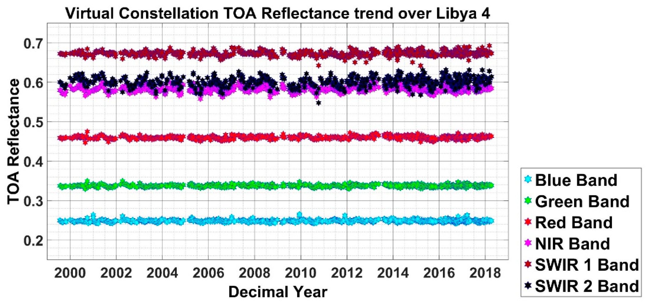
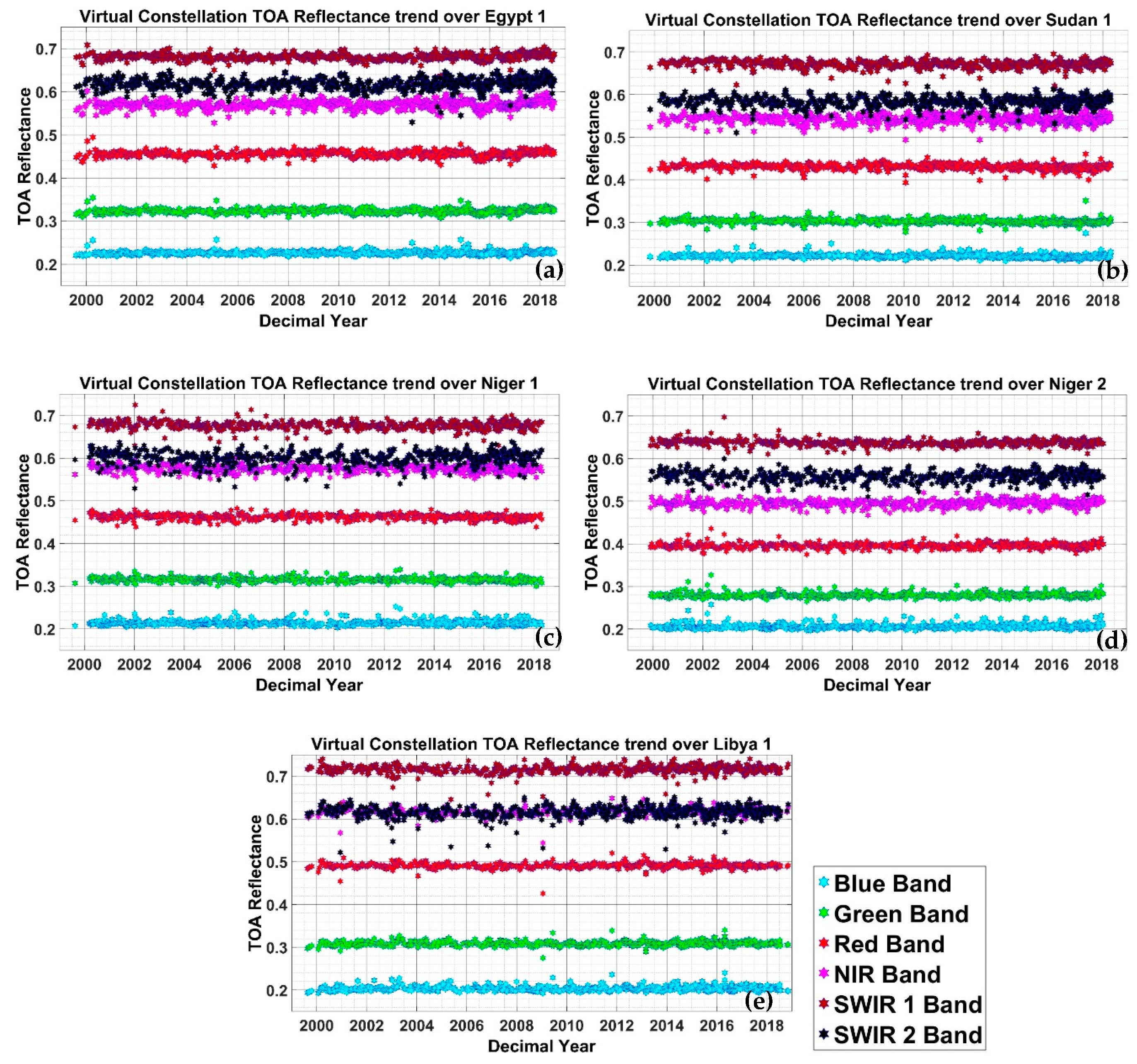
The work analyzed the TOA reflectance time series of six PICS (Libya 4, Libya 1, Niger 1, Niger 2, Egypt 1 and Sudan 1) using four sensors (Landsat 7 ETM+, Landsat 8 OLI, Terra MODIS and Sentinel-2A MSI). Initially, individual sensor time series were analyzed. However, this approach led to contradictory conclusions about a site’s temporal stability in corresponding bands among the four sensors. Inconclusive result generated by the traditional method (individual sensor-based trend analysis) is due to the time series period being different among the sensors—each sensor did not possess a common “start” time due to differences in launch date. In order to overcome these limitations, a homogenization process was performed, that is, a Virtual Constellation with the four sensors was created by combining the individual sensor time series datasets pre-processed to minimize all differences in the sensor response. A beneficial side effect of the homogenization process is a significantly increased temporal resolution of the dataset, which should allow quicker detection of small changes in TOA reflectance.

The new approach presented in this paper is robust compared to the traditional single-sensor approach, as it is not constrained by the limitations imposed by sensor design and/or operating characteristics (e.g., temporal coverage, spatial resolution, geometric and radiometric calibration accuracy, on-orbit calibration variability etc.) or by the statistical behavior of the resulting time series dataset. The VC approach can be used in trend detection not only for the selected PICS but for any PICS used by the sensor calibration community. The addition of sensors to the VC with higher temporal and spatial resolution may make this analysis more powerful.

Based on the results of the homogenized dataset analysis, it can be concluded that the Libya 4 and Egypt 1 PICS are temporally stable in the six reflective band ranges common to the four sensors. In contrast, the Sudan 1 PICS data indicate the presence of a decreasing monotonic trend in all common bands except SWIR 2; a decreasing monotonic trend is also indicated statistically in the Niger 1 Green and Red band datasets; The Niger 2 PICS data indicate an increasing monotonic trend only in the Blue band; An increasing monotonic trend is also indicated by the statistical test in the Libya 1 NIR band dataset.

The analysis presented here suggests there is sufficient statistical evidence to conclude that with respect to common spectral band ranges among the four sensors, some of the PICS are indicating monotonic trends in some specific bands. However, these trends do not suggest that the sites are changing greatly over time. The changes detected in this analysis are generally quite small to be considered physically significant. The stability requirement of PICS based on each of the Satellite Sensor mission is an important aspect to consider. For example, the highest temporal change detected in all evaluated sites was in the Blue band for Sudan 1; the percentage change in mean TOA reflectance between the periods 1999–2012 and 2013–2018 is approximately 0.8%. This amount of temporal change may be ignored by some sensors, whereas it may not be acceptable for calibration of others due its associated uncertainties. For other spectral bands of this site, as well as for other sites, the change ranged from 0.14% to 0.65%. These changes are less than the stated mission requirements (e.g., 5% calibration uncertainty for MODIS, 2% calibration uncertainty for OLI), therefore, the evaluated sites are safely considered as a viable source of calibration. However, if any sensor demonstrates less calibration uncertainty (e.g., <0.1%), the Sudan 1 site should not be used. From this analysis, it can be stated that despite very minor changes, all of the selected PICS can be used for calibration and performance monitoring of the sensors considered in this work.

The analysis presented here could be extended to determine whether the official CEOS recommended PICS exhibit temporal stability at this time and whether they maintain temporal stability over time. Overall, this work has demonstrated that even with the slight changes detected at some of the SDSU PICS, they are suitable for use in long-term monitoring of sensor performance.

References

1. Yang, J.; Gong, P.; Fu, R.; Zhang, M.; Chen, J.; Liang, S.; Xu, B.; Shi, J.; Dickinson, R. The role of satellite remote sensing in climate change studies. Nat. Clim. Chang. 2013, 3, 875. [Google Scholar] [CrossRef]
2. Thome, K.J.; Arai, K.; Tsuchida, S.; Biggar, S.F. Vicarious calibration of ASTER via the reflectance-based approach. IEEE Trans. Geosci. Remote Sens. 2008, 46, 3285–3295. [Google Scholar] [CrossRef]
3. Chander, G.; Angal, A.; Choi, T.; Xiong, X. Radiometric cross-calibration of EO-1 ALI with L7 ETM+ and Terra MODIS sensors using near-simultaneous desert observations. IEEE J. Sel. Top. Appl. Earth Obs. Remote Sens. 2013, 6, 386–399. [Google Scholar] [CrossRef]
4. Bhatt, R.; Doelling, D.R.; Wu, A.; Xiong, X.; Scarino, B.R.; Haney, C.O.; Gopalan, A. Initial stability assessment of S-NPP VIIRS reflective solar band calibration using invariant desert and deep convective cloud targets. Remote Sens. 2014, 6, 2809–2826. [Google Scholar] [CrossRef]
5. Helder, D.; Thome, K.J.; Mishra, N.; Chander, G.; Xiong, X.; Angal, A.; Choi, T. Absolute radiometric calibration of Landsat using a pseudo invariant calibration site. IEEE Trans. Geosci. Remote Sens. 2013, 51, 1360–1369. [Google Scholar] [CrossRef]
6. Chander, G.; Christopherson, J.; Stensaas, G.; Teillet, P. Online catalog of world-wide test sites for the post-launch characterization and calibration of optical sensors. In Proceedings of the 58th International Astronautical Congress 2007, Hyderabad, India, 24–28 September 2007. [Google Scholar]
7. Angal, A.; Xiong, X.; Choi, T.; Chander, G.; Wu, A. Using the Sonoran and Libyan Desert test sites to monitor the temporal stability of reflective solar bands for Landsat 7 enhanced thematic mapper plus and Terra moderate resolution imaging spectroradiometer sensors. J. Appl. Remote Sens. 2010, 4, 043525. [Google Scholar]
8. Yamamoto, H.; Kamei, A.; Nakamura, R.; Tsuchida, S. Long-term cross-calibration of the Terra ASTER and MODIS over the CEOS calibration sites. In Proceedings of the Earth Observing Systems XVI, San Diego, CA, USA, 13 September 2011. [Google Scholar]
9. Govaerts, Y.M.; Clerici, M. Evaluation of radiative transfer simulations over bright desert calibration sites. IEEE Trans. Geosci. Remote Sens. 2004, 42, 176–187. [Google Scholar] [CrossRef]
10. Govaerts, Y.M.; Clerici, M.; Clerbaux, N. Operational calibration of the Meteosat radiometer VIS band. IEEE Trans. Geosci. Remote Sens. 2004, 42, 1900–1914. [Google Scholar] [CrossRef]
11. Teillet, P.; Barsi, J.; Chander, G.; Thome, K. Prime candidate earth targets for the post-launch radiometric calibration of space-based optical imaging instruments. In Proceedings of the Earth Observing Systems XII, San Diego, CA, USA, 5 October 2007. [Google Scholar]
12. Chander, G.; Angal, A.; Xiong, X.J.; Helder, D.L.; Mishra, N.; Choi, T.J.; Wu, A. Preliminary assessment of several parameters to measure and compare usefulness of the CEOS reference pseudo-invariant calibration sites. In Proceedings of the Sensors, Systems and Next-Generation Satellites XIV, Toulouse, France, 20–23 September 2010. [Google Scholar]
13. Morstad, D.L.; Helder, D.L. Use of pseudo-invariant sites for long-term sensor calibration. In Proceedings of the IGARSS 2008–2008 IEEE International Geoscience and Remote Sensing Symposium, Boston, MA, USA, 8–11 July 2008. [Google Scholar]
14. Chander, G.; Xiong, X.J.; Choi, T.J.; Angal, A. Monitoring on-orbit calibration stability of the Terra MODIS and Landsat 7 ETM+ sensors using pseudo-invariant test sites. Remote Sens. Environ. 2010, 114, 925–939. [Google Scholar] [CrossRef]
15. Virtual Constellations. Available online: http://ceos.org/ourwork/virtual-constellations/ (accessed on 1 January 2019).
16. Claverie, M.; Ju, J.; Masek, J.G.; Dungan, J.L.; Vermote, E.F.; Roger, J.-C.; Skakun, S.V.; Justice, C. The Harmonized Landsat and Sentinel-2 surface reflectance data set. Remote Sens. Environ. 2018, 219, 145–161. [Google Scholar] [CrossRef]
17. Helder, D.; Markham, B.; Morfitt, R.; Storey, J.; Barsi, J.; Gascon, F.; Clerc, S.; LaFrance, B.; Masek, J.; Roy, D. Observations and Recommendations for the Calibration of Landsat 8 OLI and Sentinel 2 MSI for improved data interoperability. Remote Sens. 2018, 10, 1340. [Google Scholar] [CrossRef]
18. Micijevic, E.; Mishra, N.; Helder, D. Assessing Long Term Stability of Landsat 5 TM, Landsat 7 ETM+ and Landsat 8 OLI. In Proceedings of the Conference on Characterization and Radiometric Calibration for Remote Sensing (CALCON), Logan, UT, USA, 21–24 August 2017. [Google Scholar]
19. USGS. Landsat Missions. Available online: https://www.usgs.gov/land-resources/nli/landsat (accessed on 1 January 2019).
20. Xiong, X.; Chiang, K.; Esposito, J.; Guenther, B.; Barnes, W. MODIS on-orbit calibration and characterization. Metrologia 2003, 40, S89. [Google Scholar] [CrossRef]
21. Angal, A.; Xiong, X.; Helder, D.; Kaewmanee, M.; Leigh, L. Assessing the calibration differences in the reflective solar bands of Terra MODIS and Landsat-7 enhanced thematic mapper plus. J. Appl. Remote Sens. 2018, 12, 044002. [Google Scholar] [CrossRef]
22. Barsi, J.A.; Markham, B.L.; Czapla-Myers, J.S.; Helder, D.L.; Hook, S.J.; Schott, J.R.; Haque, M.O. Landsat-7 ETM+ radiometric calibration status. In Proceedings of the Earth Observing Systems XXI, San Diego, CA, USA, 19 September 2016. [Google Scholar]
23. Markham, B.; Barsi, J.; Kvaran, G.; Ong, L.; Kaita, E.; Biggar, S.; Czapla-Myers, J.; Mishra, N.; Helder, D. Landsat-8 operational land imager radiometric calibration and stability. Remote Sens. 2014, 6, 12275–12308. [Google Scholar] [CrossRef]
24. Micijevic, E.; Haque, M.O.; Mishra, N. Radiometric calibration updates to the Landsat collection. In Proceedings of the Earth Observing Systems XXI, San Diego, CA, USA, 28 August–1 September 2016. [Google Scholar]
25. Xiong, X.; Angal, A.; Barnes, W.L.; Chen, H.; Chiang, V.; Geng, X.; Li, Y.; Twedt, K.; Wang, Z.; Wilson, T. Updates of Moderate Resolution Imaging Spectroradiometer on-orbit calibration uncertainty assessments. J. Appl. Remote Sens. 2018, 12, 034001. [Google Scholar] [CrossRef]
26. Gascon, F.; Bouzinac, C.; Thépaut, O.; Jung, M.; Francesconi, B.; Louis, J.; Lonjou, V.; Lafrance, B.; Massera, S.; Gaudel-Vacaresse, A. Copernicus Sentinel-2A calibration and products validation status. Remote Sens. 2017, 9, 584. [Google Scholar] [CrossRef]
27. Barsi, J.A.; Alhammoud, B.; Czapla-Myers, J.; Gascon, F.; Haque, M.O.; Kaewmanee, M.; Leigh, L.; Markham, B.L. Sentinel-2A MSI and Landsat-8 OLI radiometric cross comparison over desert sites. Eur. J. Remote Sens. 2018, 51, 822–837. [Google Scholar] [CrossRef]
28. ESA Sentinel Online. Available online: https://earth.esa.int/web/sentinel/technical-guides/sentinel-2-msi/performance (accessed on 1 January 2019).
29. Helder, D.L.; Basnet, B.; Morstad, D.L. Optimized identification of worldwide radiometric pseudo-invariant calibration sites. Can. J. Remote Sens. 2010, 36, 527–539. [Google Scholar] [CrossRef]
30. Mishra, N.; Helder, D.; Angal, A.; Choi, J.; Xiong, X. Absolute calibration of optical satellite sensors using Libya 4 pseudo invariant calibration site. Remote Sens. 2014, 6, 1327–1346. [Google Scholar] [CrossRef]
31. Vuppula, H. Normalization of Pseudo-invariant Calibration Sites for Increasing the Temporal Resolution and Long-Term Trending. Master’s Thesis, South Dakota State University, Brookings, SD, USA, 2017. [Google Scholar]
32. Lyapustin, A.; Wang, Y.; Korkin, S.; Huang, D. MODIS Collection 6 MAIAC algorithm. Atmos. Meas. Tech. 2018, 11, 5741–5765. [Google Scholar] [CrossRef] [Green Version]
33. USGS. Landsat 8 (L8) Data Users Handbook; EROS: Sioux Falls, South Dakota, 2016; p. 106.
34. USGS. Landsat 7 Science Data Users Handbook; USGS: Washington, DC, USA, 2011; p. 186.
35. Neckel, H.; Labs, D. The solar radiation between 3300 and 12,500 Angstorms. Sol. Phys. 1984, 90, 205–258. [Google Scholar] [CrossRef]
36. Smith, E.V.; Gottlieb, D.M. Solar flux and its variations. Space Sci. Rev. 1974, 16, 771–802. [Google Scholar] [CrossRef]
37. Thuillier, G.; Hersé, M.; Simon, P.; Mandel, H.; Gillotay, D. Observation of the solar spectral irradiance from 200 nm to 870 nm during the ATLAS 1 and ATLAS 2 missions by the SOLSPEC spectrometer. Metrologia 1998, 35, 689. [Google Scholar] [CrossRef]
38. Strabala, K.I. MODIS Cloud Mask User’s Guide; University of Wisconsin-Madison: Madison, WI, USA, 2005. [Google Scholar]
39. Farhad, M.M. Cross Calibration and Validation of Landsat 8 OLI and Sentinel 2A MSI. Master’s Thesis, South Dakota State University, Brookings, SD, USA, 2018. [Google Scholar]
40. Mendes, M.; Pala, A. Type I error rate and power of three normality tests. Pak. J. Inf. Technol. 2003, 2, 135–139. [Google Scholar]
41. Yap, B.W.; Sim, C.H. Comparisons of various types of normality tests. J. Stat. Comput. Simul. 2011, 81, 2141–2155. [Google Scholar] [CrossRef]
42. Angal, A.; Xiong, X.; Choi, T.; Chander, G.; Mishra, N.; Helder, D.L. Impact of Terra MODIS Collection 6 on long-term trending comparisons with Landsat 7 ETM+ reflective solar bands. Remote Sens. Lett. 2013, 4, 873–881. [Google Scholar] [CrossRef]
43. Hirsch, R.M.; Slack, J.R. A nonparametric trend test for seasonal data with serial dependence. Water Resour. Res. 1984, 20, 727–732. [Google Scholar] [CrossRef]
44. Meals, D.W.; Spooner, J.; Dressing, S.A.; Harcum, J.B. Statistical Analysis for Monotonic Trends; Tertra Tech Inc.: Fairfax, VA, USA, 2011. [Google Scholar]
45. Thas, O.; Van Vooren, L.; Ottoy, J. Selection of nonparametric methods for monotonic trend detection in water quality. J. Am. Water Res. Assoc. 2007, 34, 347–357. [Google Scholar] [CrossRef]
46. Posada, D.; Buckley, T.R. Model selection and model averaging in phylogenetics: Advantages of Akaike information criterion and Bayesian approaches over likelihood ratio tests. Syst. Boil. 2004, 53, 793–808. [Google Scholar] [CrossRef]
Figure 1. Relative Spectral Response of four Sensors for six analogous spectral bands.
Remotesensing 11 01502 g001
Figure 2. 3% Stable Optimal Regions (white masks) and Rectangular region of interests (ROIs) (blue rectangle) within SDSU IPLAB PICS (Niger 1, Niger 2, Libya 1, Libya 4, Egypt 1 and Sudan 1).
Remotesensing 11 01502 g002
Figure 3. Histogram of ETM+ BRDF-corrected Mean TOA Reflectance of Libya 4; (a) Blue band; (b) SWIR2 band.
Remotesensing 11 01502 g003
Figure 4. Temporal trend of BRDF-corrected TOA Reflectance over Libya 4 Site [L7 ETM+, Terra MODIS, L8 OLI and S2A MSI]. Blue (a), Green (b), Red (c), NIR (d), SWIR 1 (e) and SWIR 2 (f) spectral bands. Note that in this figure the scaling adjustment factor has not been applied yet.
Remotesensing 11 01502 g004aRemotesensing 11 01502 g004b
Figure 5. Temporal trend of BRDF-corrected Scaling Adjusted TOA reflectance over Libya 4 site (L7 ETM+, Terra MODIS, L8-OLI, S2A-MSI) in (a) blue band; (b) Green band; (c) Red band; (d) NIR band; (e) SWIR 1 band; (f) SWIR 2 band.
Remotesensing 11 01502 g005aRemotesensing 11 01502 g005b
Figure 6. Virtual constellation – homogenized 4 sensor’s TOA reflectance trends for the 6 spectrally matched bands over Libya 4 site.
Remotesensing 11 01502 g006
Figure 7. Homogenized TOA reflectance trends of Egypt 1 (a), Sudan 1 (b), Niger 1(c), Niger 2 (d) and Libya 1(e) PICS.
Remotesensing 11 01502 g007