Obtaining High-Resolution Seabed Topography and Surface Details by Co-Registration of Side-Scan Sonar and Multibeam Echo Sounder Images


Abstract
1. Introduction
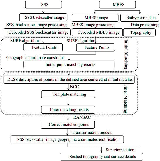
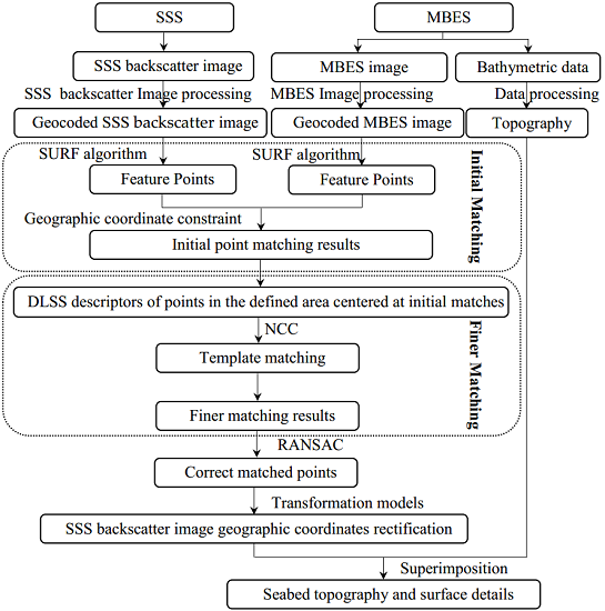
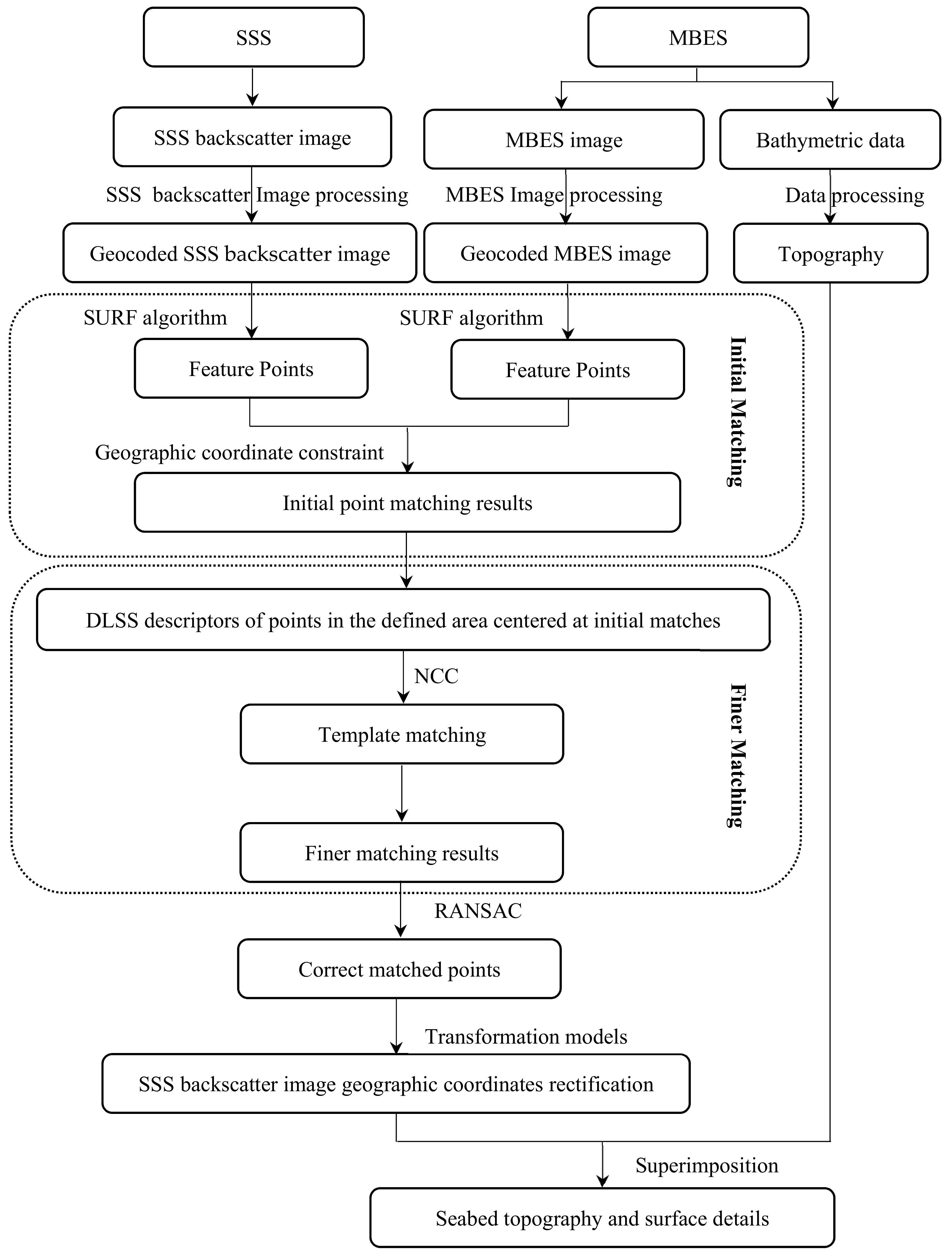
2. Method
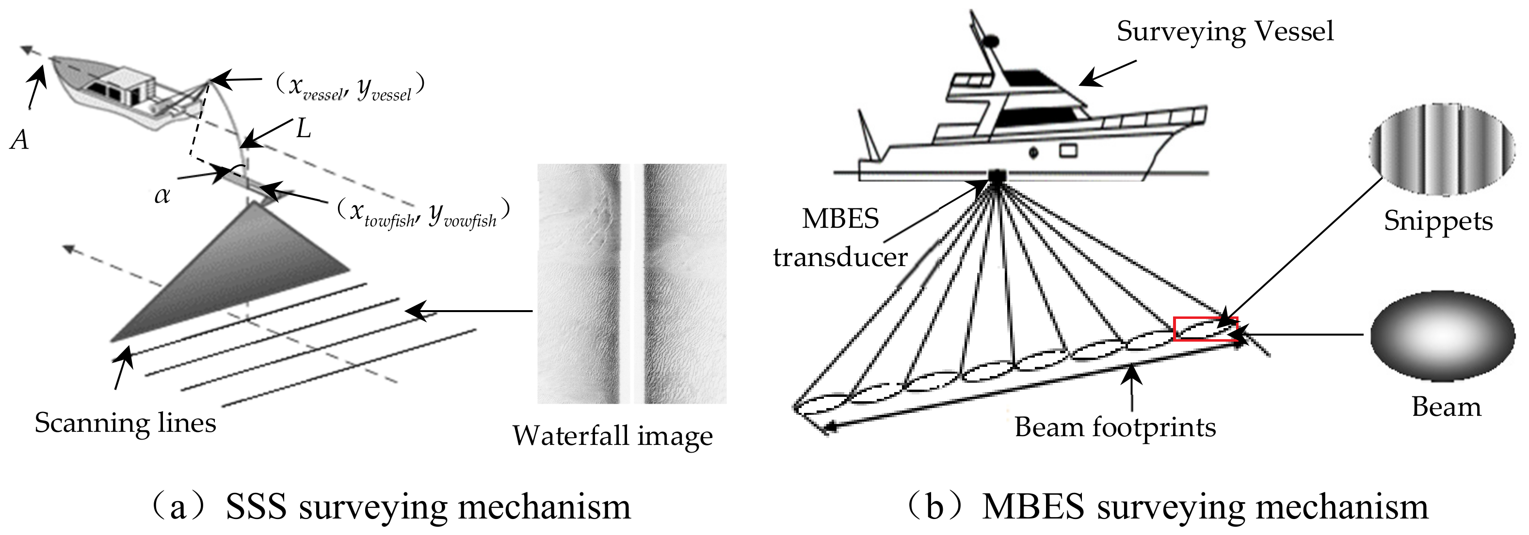
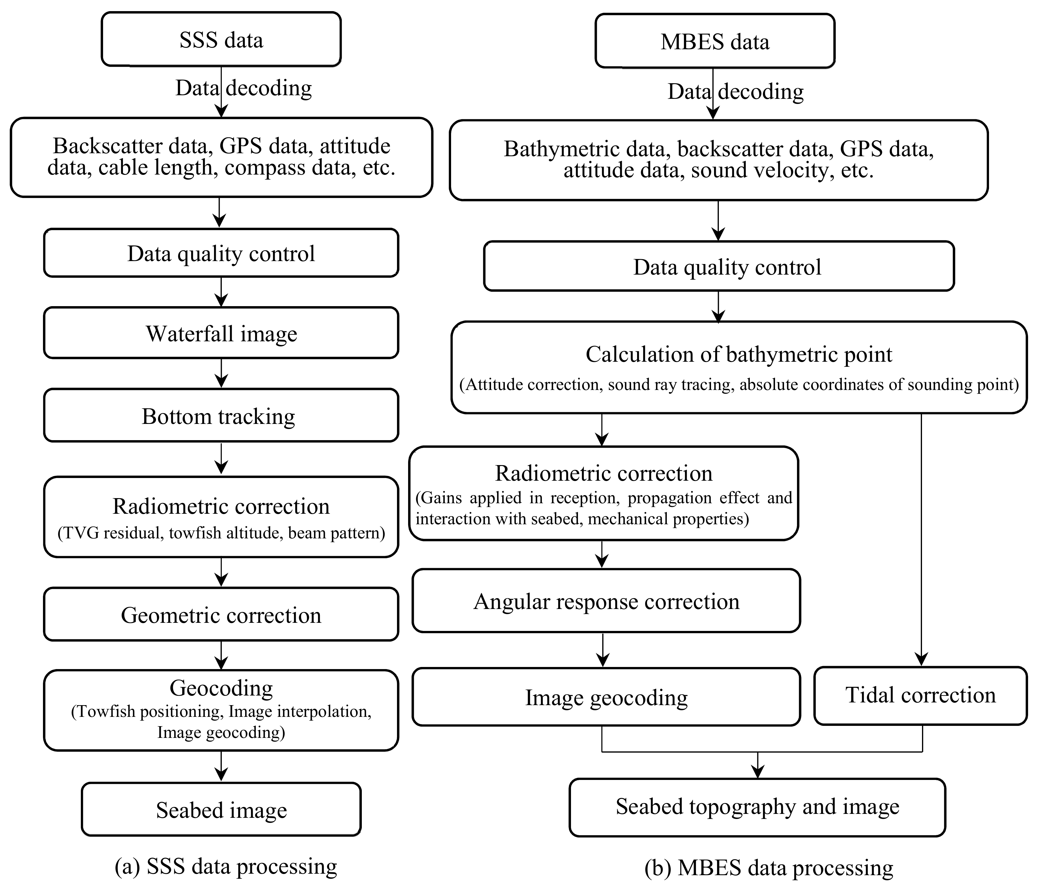
2.1. SSS and MBES Data Processing
2.2. SSS and MBES Image Matching
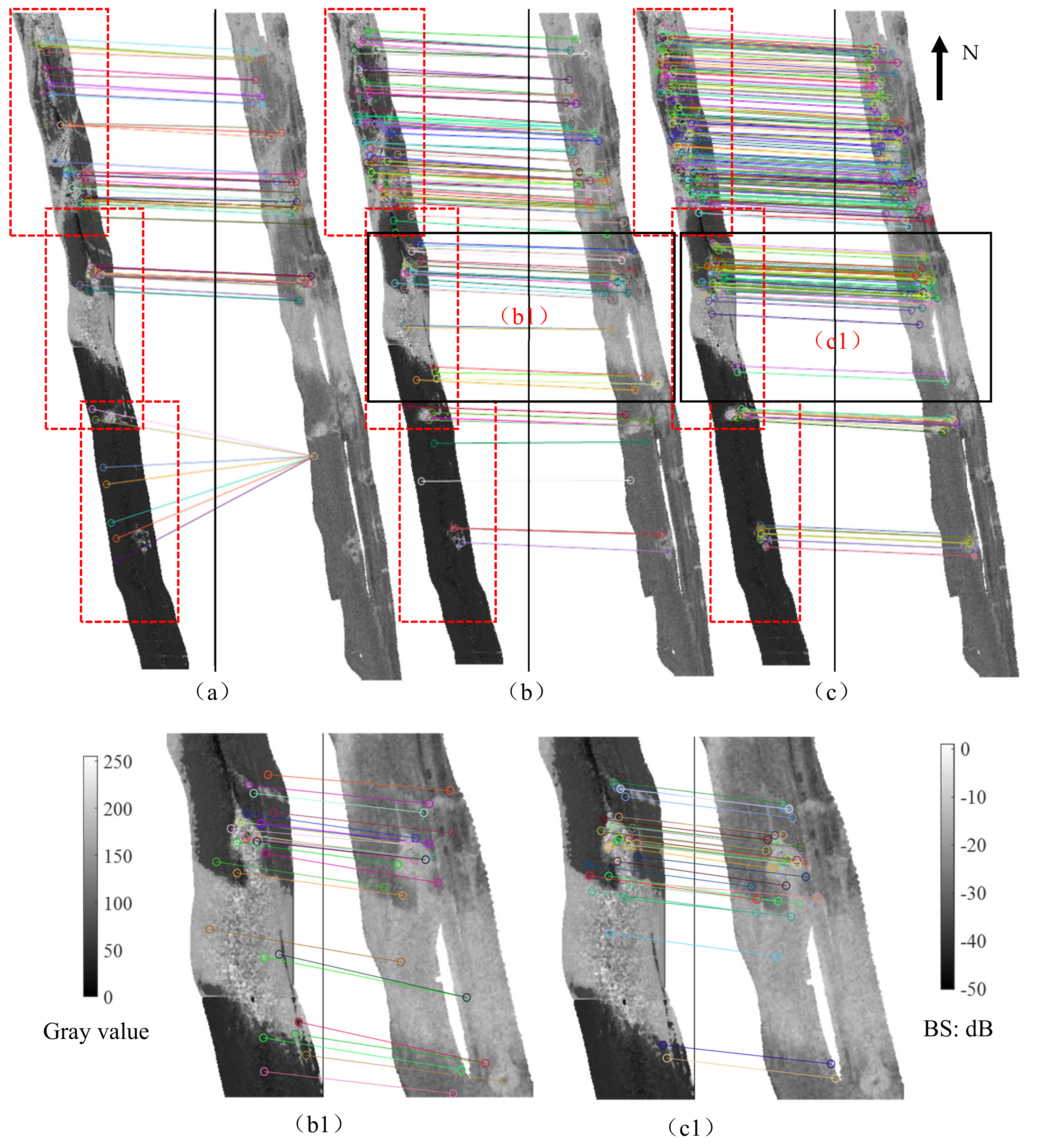
2.2.1. Initial Image Matching Using SURF Algorithm with Image Geographic Coordinate Constraint
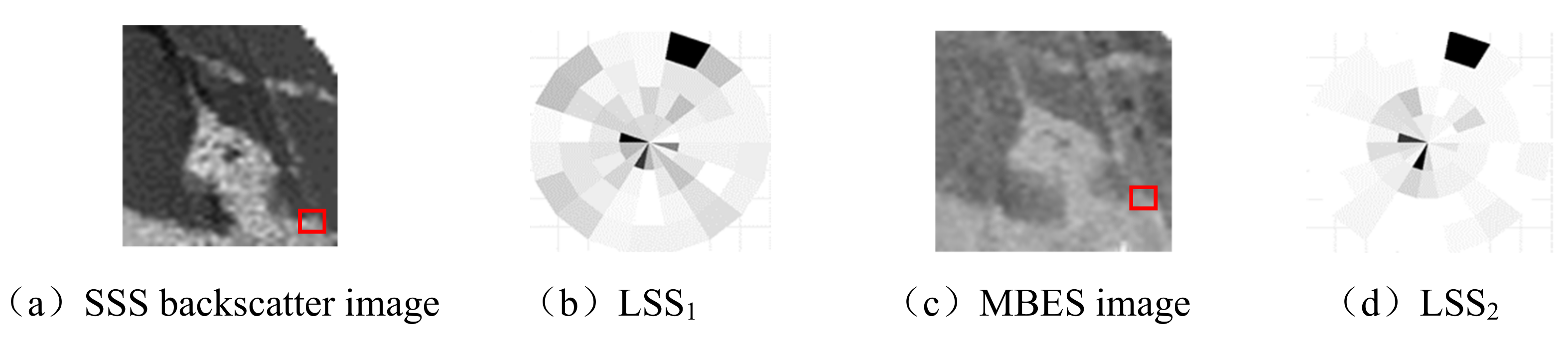
2.2.2. Finer Image Matching Using DLSS Descriptors
2.3. SSS Backscatter Image Geographic Coordinates Rectification Based on the Matched Points
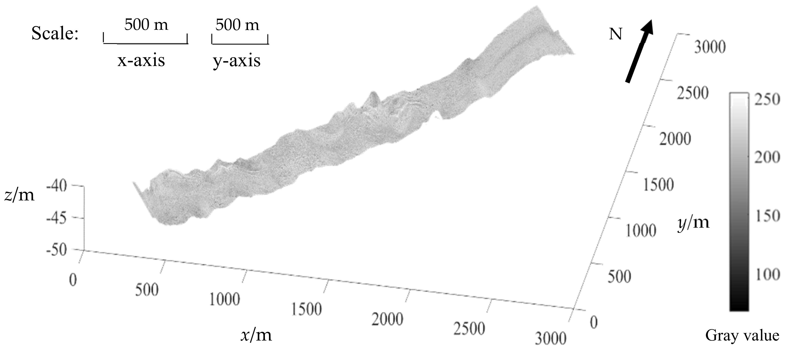
2.4. Superimposition of Rectified SSS Backscatter Image on MBES Terrain
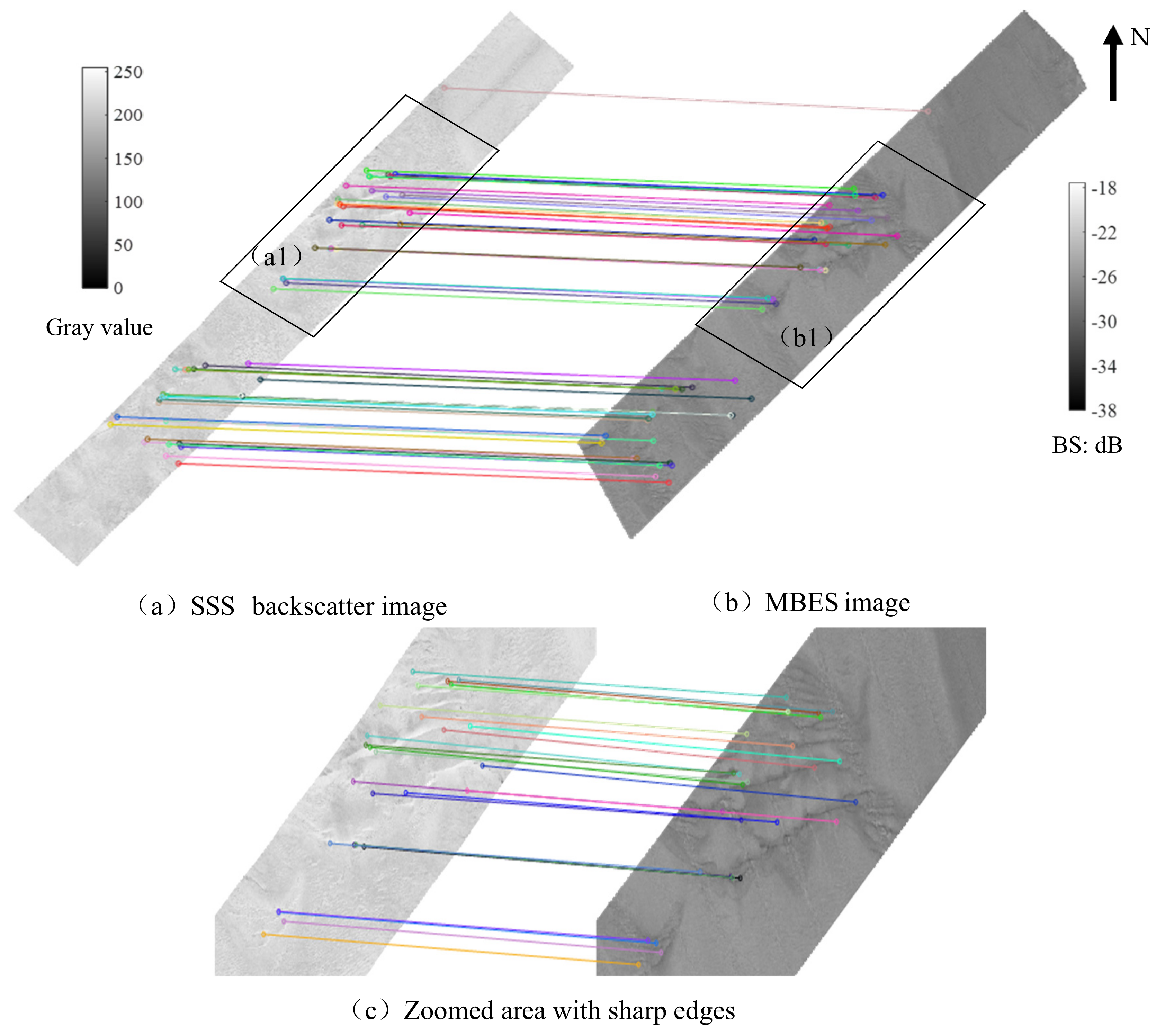
3. Experiments and Results
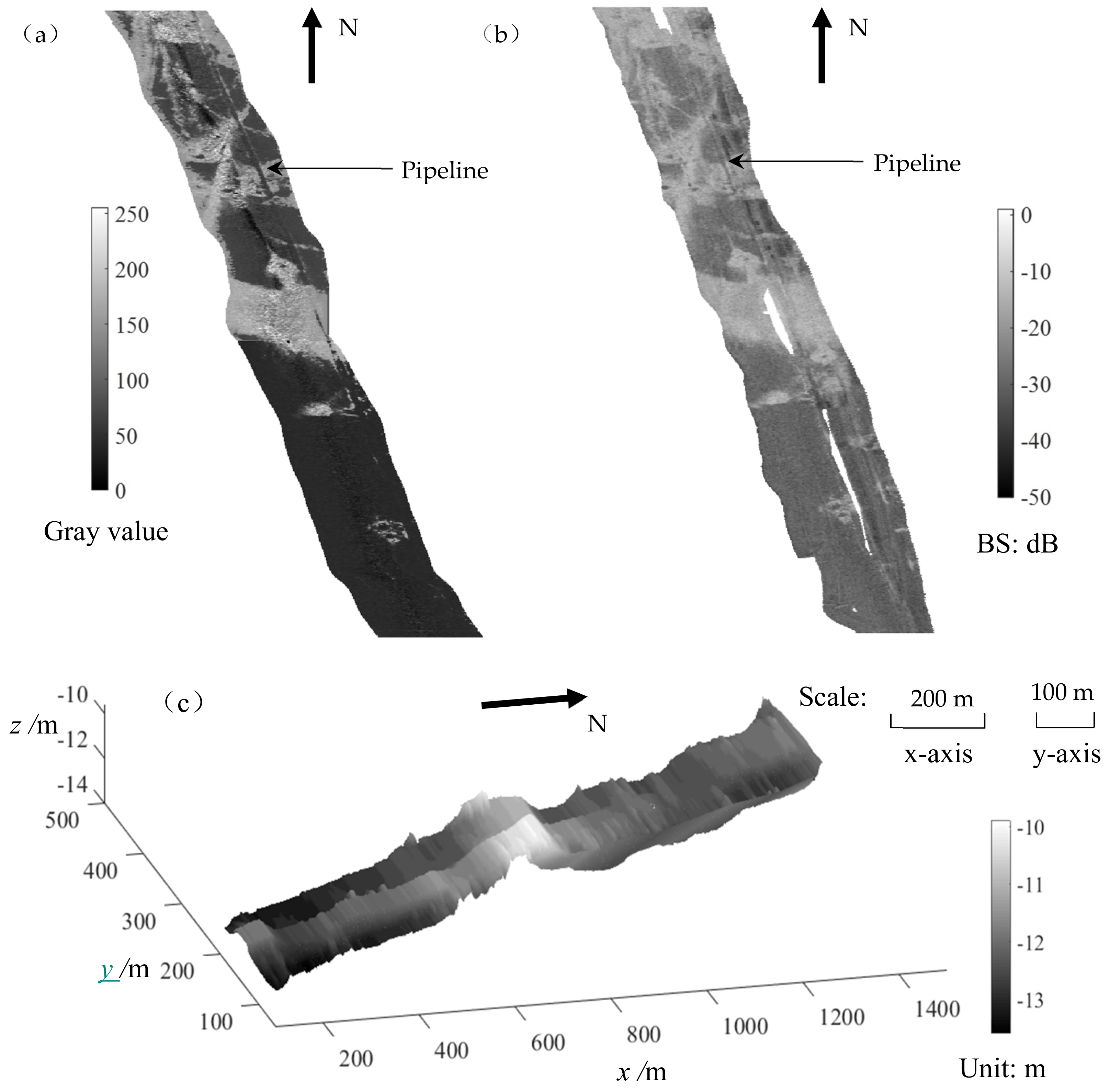
3.1. Experimental Data
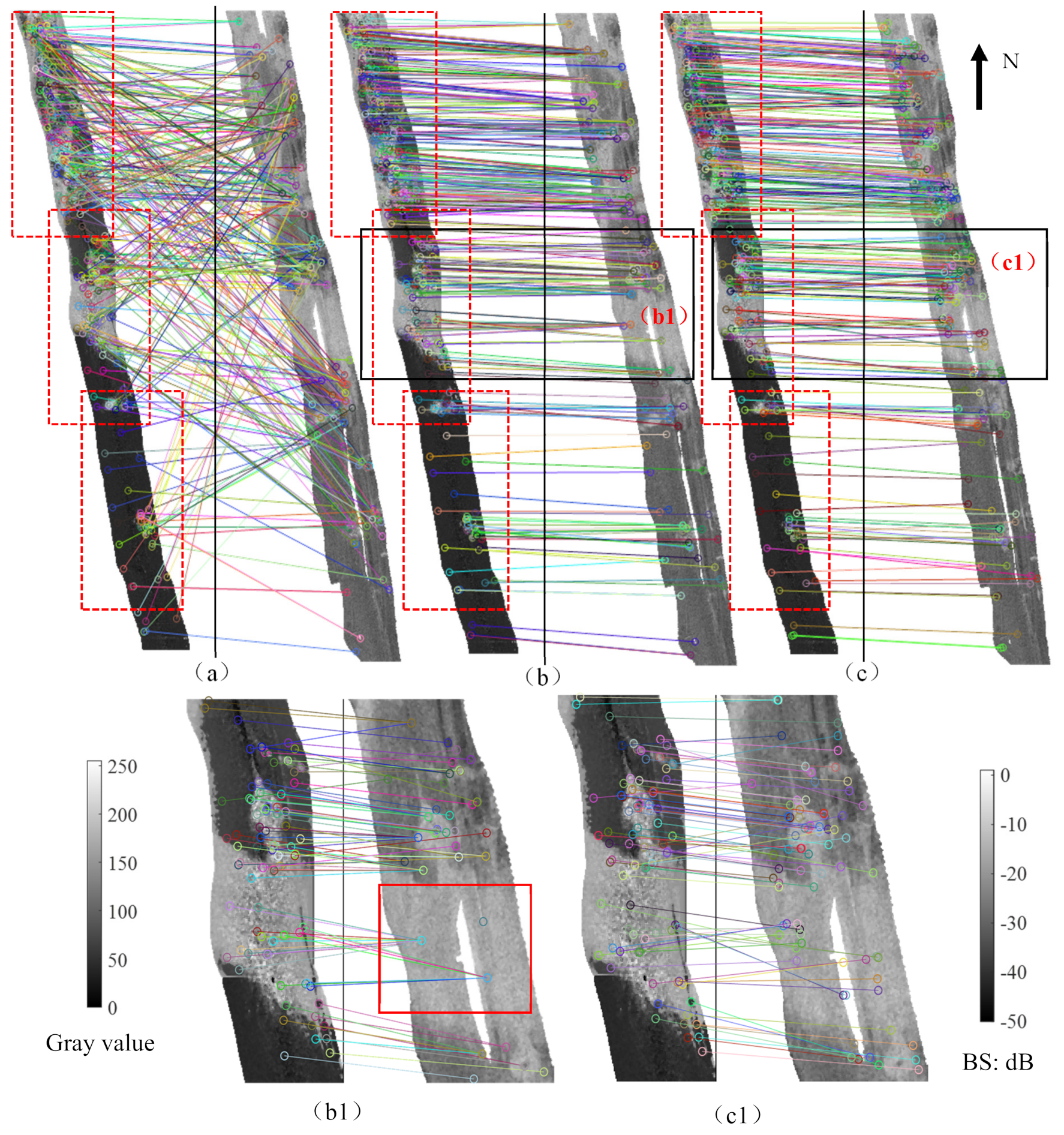
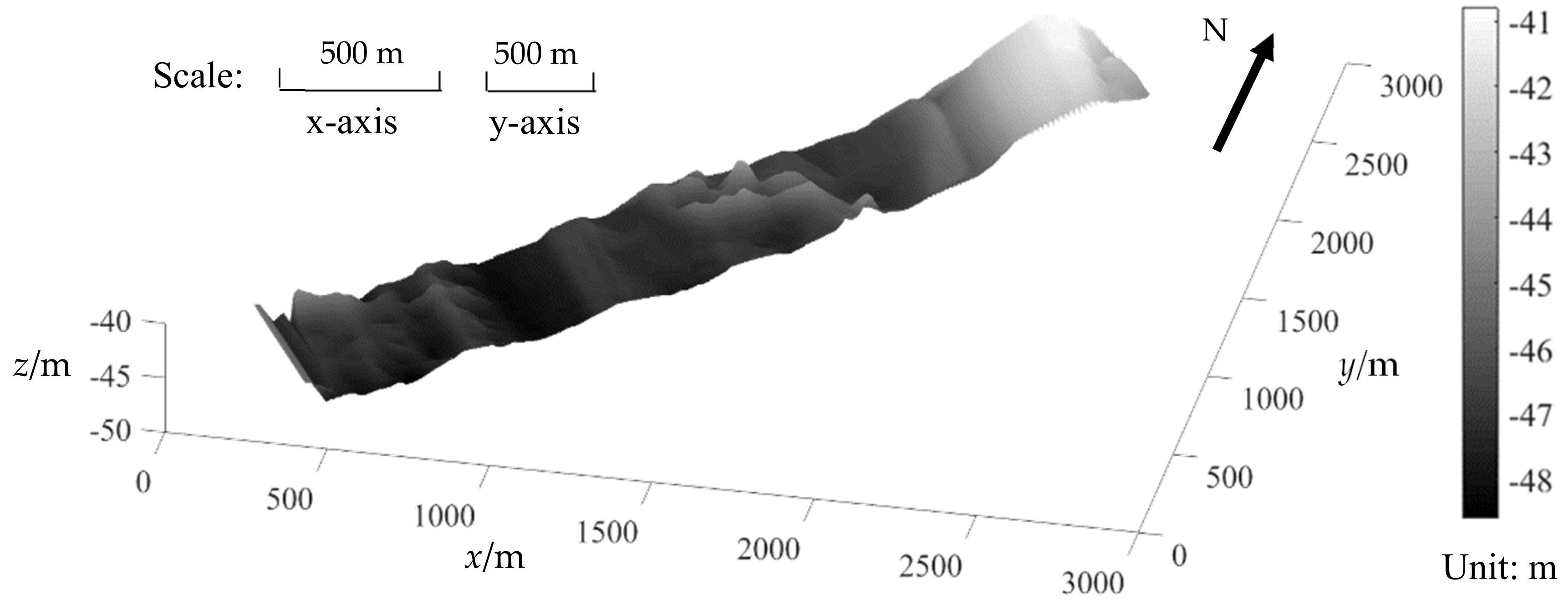
3.2. Experimental Procedure and Results
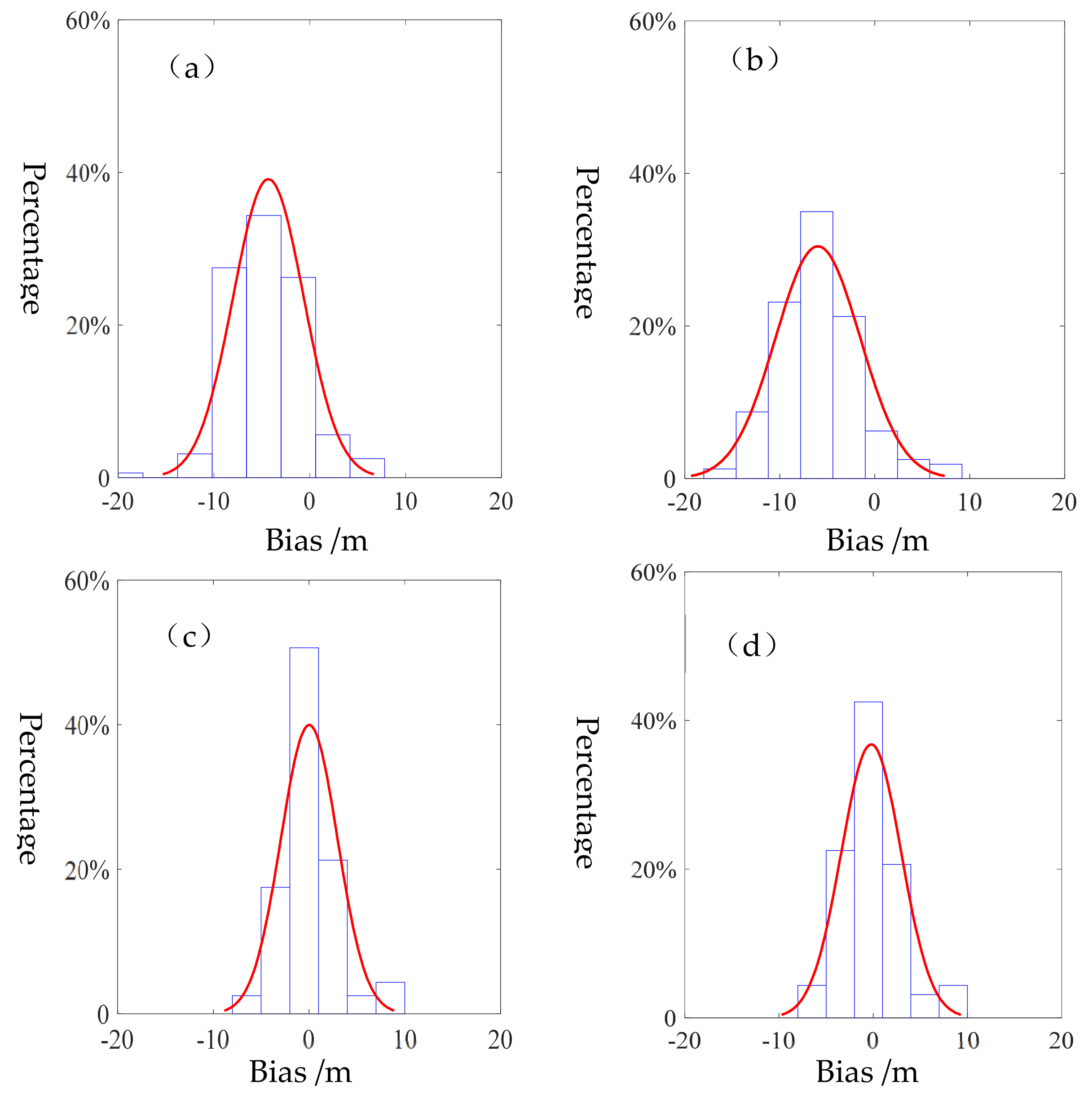
4. Evaluation and Analysis
5. Discussions
5.1. Determination of the Threshold Dis and Searching Radius
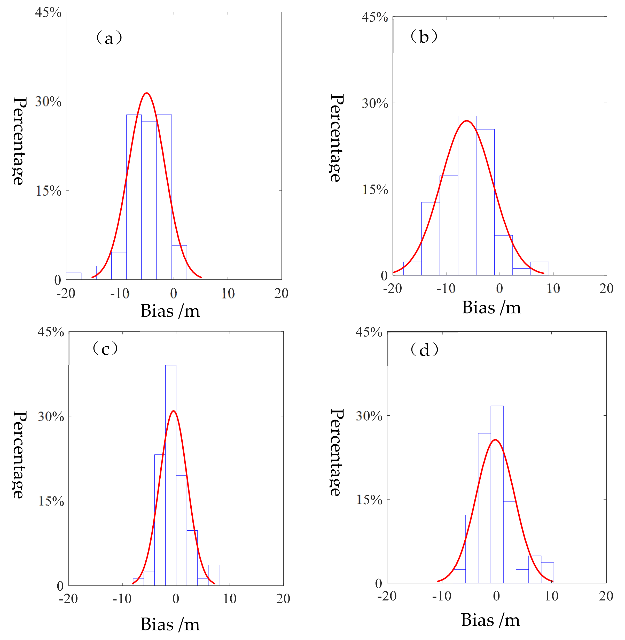
5.2. Method Repeatability: Applicability of the Proposed Method in another Situation
5.3. Sonar Frequencies
6. Conclusions
Author Contributions
Funding
Acknowledgments
Conflicts of Interest
References
- Mayer, L.; Jakobsson, M.; Allen, G.; Dorschel, B.; Falconer, R.; Ferrini, V.; Lamarche, G.; Snaith, H.; Weatherall, P. The Nippon Foundation—GEBCO Seabed 2030 Project: The Quest to See the World’s Oceans Completely Mapped by 2030. Geosciences 2018, 8, 63. [Google Scholar] [CrossRef]
- DeSanto, J.B.; Sandwell, D.T.; Chadwell, C.D. Seafloor geodesy from repeated sidescan sonar surveys. J. Geophys. Res. Solid Earth 2016, 121, 4800–4813. [Google Scholar] [CrossRef]
- Powers, J.; Brewer, S.K.; Long, J.M.; Campbell, T. Evaluating the use of side-scan sonar for detecting freshwater mussel beds in turbid river environments. Hydrobiologia 2015, 743, 127–137. [Google Scholar] [CrossRef]
- Lurton, X. Forty years of progress in multibeam echosounder technology for ocean investigation. J. Acoust. Soc. Am. 2017, 141, 3948. [Google Scholar] [CrossRef]
- Blondel, P. The Handbook of Sidescan Sonar; Springer: Berlin/Heidelberg, Germany; New York, NY, USA, 2009; ISBN 978-3-540-42641-7. [Google Scholar]
- Lurton, X.; Jackson, D. An Introduction to Underwater Acoustics, 2nd ed.; Springer-Praxis: New York, NY, USA, 2008; ISBN 3540429670. [Google Scholar]
- Tamsett, D.; Hogarth, P. Sidescan sonar beam function and seabed backscatter functions from trace amplitude and vehicle roll data. IEEE J. Ocean. Eng. 2015, 411, 155–163. [Google Scholar] [CrossRef]
- Bell, J.M.; Linnett, L.M. Simulation and analysis of synthetic sidescan sonar images. IEE Proc. Radar Sonar Navig. 1997, 144, 219–226. [Google Scholar] [CrossRef]
- Cobra, D.T.; Oppenheim, A.V.; Jaffe, J.S. Geometric distortions in side-scan sonar images: A procedure for their estimation and correction. IEEE J. Ocean. Eng. 1992, 17, 252–268. [Google Scholar] [CrossRef]
- Clarke, J. Dynamic Motion Residuals in Swath Sonar Data: Ironing out the Creases. Int. Hydrogr. Rev. 2003, 4, 6–23. [Google Scholar]
- Cervenka, P.; Moustier, C.D.; Lonsdale, P.F. Geometric corrections on sidescan sonar images based on bathymetry: Application with SeaMARC II and Sea Beam data. Mar. Geophys. Res. 1995, 17, 217–219. [Google Scholar] [CrossRef]
- Cervenka, P.; de Moustier, C. Postprocessing and corrections of bathymetry derived from sidescan sonar systems: Application with SeaMARC II. IEEE J. Ocean. Eng. 1994, 19, 619–629. [Google Scholar] [CrossRef]
- Coiras, E.; Petillot, Y.; Lane, D.M. Multiresolution 3-D reconstruction from side-scan sonar images. IEEE Trans. Image Process. 2007, 16, 382–390. [Google Scholar] [CrossRef] [PubMed]
- Fezzani, R.; Zerr, B.; Mansour, A.; Legris, M.; Vrignaud, C. Fusion of Swath Bathymetric Data: Application to AUV Rapid Environment Assessment. IEEE J. Ocean. Eng. 2019, 44, 111–120. [Google Scholar] [CrossRef]
- Stateczny, A.; Gronska, D.; Motyl, W. HydroDron—New step for professional hydrography for restricted waters. BGC Geomat. 2018, 226–230. [Google Scholar] [CrossRef]
- Crawford, A.; Connors, W. Performance Evaluation of a 3-D Sidescan Sonar for Mine Countermeasures. In Proceedings of the OCEANS 2018 MTS, Charleston, SC, USA, 22–25 October 2018. [Google Scholar]
- Ai, Y.; Armstrong, S.; Fleury, D. Evaluation of the Klein Hydrochart 3500 Interferometric Bathymetry Sonar for Noaa Sea Floor Mapping. In Proceedings of the OCEANS 2015 MTS, Washington, DC, USA, 18–21 May 2015. [Google Scholar]
- Brisson, L.; Wolfe, D.; Staley, M. Interferometric swath bathymetry for large scale shallow water hydrographic surveys. In Proceedings of the Canadian Hydrographic Conference, St. John’s, NL, Canada, 14–17 April 2014. [Google Scholar]
- Schimel, A.C.; Beaudoin, J.; Parnum, I.; LeBas, T.P.; Schmidt, V.; Keith, G.; Ierodiaconou, D. Multibeam sonar backscatter data processing. Mar. Geophys. Res. 2018, 39, 121–137. [Google Scholar] [CrossRef]
- Lucieer, V.; Roche, M.; Degrendele, K.; Malik, M.; Dolan, M.; Lamarche, G. User expectations for multibeam echo sounders backscatter strength data-looking back into the future. Mar. Geophys. Res. 2018, 39, 23–40. [Google Scholar] [CrossRef]
- LeBas, T.P.; Huvenne, V. Acquisition and processing of backscatter data for habitat mapping–comparison of multibeam and sidescan systems. Appl. Acoust. 2009, 70, 1248–1257. [Google Scholar] [CrossRef]
- Mitchell, G.A.; Orange, D.L.; Gharib, J.J.; Kennedy, P. Improved detection and mapping of deepwater hydrocarbon seeps: Optimizing multibeam echosounder seafloor backscatter acquisition and processing techniques. Mar. Geophys. Res. 2018, 39, 323–347. [Google Scholar] [CrossRef]
- Fakiris, E.; Blondel, P.; Papatheodorou, G.; Christodoulou, D.; Dimas, X.; Georgiou, N.; Kordella, S.; Dimitriadis, C.; Rzhanov, Y.; Geraga, M.; et al. Multi-Frequency, Multi-Sonar Mapping of Shallow Habitats—Efficacy and Management Implications in the National Marine Park of Zakynthos, Greece. Remote Sens. 2019, 11, 461. [Google Scholar] [CrossRef]
- LeBas, T.P.; Mason, D.C. Automatic registration of TOBI side-scan sonar and multi-beam bathymetry images for improved data fusion. Mar. Geophys. Res. 1997, 19, 163–176. [Google Scholar] [CrossRef]
- Yang, F.; Wu, Z.; Du, Z.; Jin, X. Co-registering and fusion of digital information of multibeam sonar and side-scan sonar. Geomat. Inf. Sci. Wuhan Univ. 2006, 31, 740–743. [Google Scholar] [CrossRef]
- Zhao, J.; Wang, A.; Guo, J. Study on fusion method of the block image of MBS and SSS. Geomat. Inf. Sci. Wuhan Univ. 2013, 38, 287–290. [Google Scholar] [CrossRef]
- Yan, J. Acquisition and superposition of the high-quality measurement information of multibeam echo sonar. Acta Geod. Et Cartogr. Sin. 2019, 48, 400. [Google Scholar] [CrossRef]
- Fakiris, E.; Papatheodorou, G. Quantification of regions of interest in swath sonar backscatter images using grey-level and shape geometry descriptors: The TargAn software. Mar. Geophys. Res. 2012, 33, 169–183. [Google Scholar] [CrossRef]
- Wang, A.; Zhang, H.; Wang, X.; Shang, X. Processing Principles of Side-scan Sonar Data for Seamless Mosaic Image. J. Geomat. 2017, 42, 26–29. [Google Scholar] [CrossRef]
- Cervenka, P.; de Moustier, C. Sidescan sonar image processing techniques. IEEE J. Ocean. Eng. 1993, 18, 108–122. [Google Scholar] [CrossRef]
- Ye, X.; Yang, H.; Li, C.; Jia, Y.; Li, P. A Gray Scale Correction Method for Side-Scan Sonar Images Based on Retinex. Remote Sens. 2019, 11, 1281. [Google Scholar] [CrossRef]
- Capus, C.G.; Banks, A.C.; Coiras, E.; Ruiz, I.T.; Smith, C.J.; Petillot, Y.R. Data correction for visualisation and classification of sidescan SONAR imagery. IET Radar Sonar Navig. 2008, 2, 155–169. [Google Scholar] [CrossRef]
- Bay, H.; Ess, A.; Tuytelaars, T.; Gool, L. Speeded-Up Robust Features (SURF). Comput. Vis. Image Underst. 2008, 110, 346–359. [Google Scholar] [CrossRef]
- Sedaghat, A.; Mohammadi, N. High-resolution image registration based on improved SURF detector and localized GTM. Int. J. Remote Sens. 2019, 40, 2576–2601. [Google Scholar] [CrossRef]
- Tola, E.; Lepetit, V.; Fua, P. Daisy: An efficient dense descriptor applied to wide-baseline stereo. IEEE Trans. Pattern Anal. Mach. Intell. 2009, 32, 815–830. [Google Scholar] [CrossRef]
- Li, J.; Hu, Q.; Ai, M.; Zhong, R. Robust feature matching via support-line voting and affine-invariant ratios. ISPRS J. Photogramm. Remote Sens. 2017, 132, 61–76. [Google Scholar] [CrossRef]
- Ye, Y.; Shen, L.; Hao, M.; Wang, J.; Xu, Z. Robust optical-to-SAR image matching based on shape properties. IEEE Geosci. Remote Sens. Lett. 2017, 14, 564–568. [Google Scholar] [CrossRef]
- Shechtman, E.; Irani, M. Matching local self-similarities across images and videos. In Proceedings of the IEEE Conference on Computer Vision and Pattern Recognition, Minneapolis, MN, USA, 17–22 June 2007; pp. 1–8. [Google Scholar]
- Fischler, M.A.; Bolles, R.C. Random sample consensus: A paradigm for model fitting with applications to image analysis and automated cartography. Commun. ACM 1981, 24, 381–395. [Google Scholar] [CrossRef]
- Chailloux, C.; Caillec, J.; Gueriot, D.; Zerr, B. Intensity-Based Block Matching Algorithm for Mosaicing Sonar Images. IEEE J. Ocean. Eng. 2011, 36, 627–645. [Google Scholar] [CrossRef]
- Zhao, J.; Wang, A.; Zhang, H.; Wang, X. Mosaic method of side-scan sonar strip images using corresponding features. IET Image Process. 2013, 7, 616–623. [Google Scholar] [CrossRef]
- Wang, A.; Zhao, J.; Guo, J.; Wang, X. Elastic Mosaic Method in Block for Side Scan Sonar Image Based on Speeded-Up Robust Features. Geomat. Inf. Sci. Wuhan Univ. 2018, 43, 697–703. [Google Scholar] [CrossRef]
- Daniel, S.; Leannec, F.L.; Roux, C.; Solaiman, B.; Maillard, E.P. Side-Scan Sonar Image Matching. IEEE J. Ocean. Eng. 1998, 23, 245–259. [Google Scholar] [CrossRef]
- Yang, L.; Jiao, Y.; Xu, J. Underwater target positioning technology of side scan sonar based on ultra short baseline. China Harb. Eng. 2017, 37, 6–9. [Google Scholar] [CrossRef]
- Feldens, P.; Schulze, I.; Papenmeier, S.; Schönke, M.; Schneider von Deimling, J. Improved Interpretation of Marine Sedimentary Environments Using Multi-Frequency Multibeam Backscatter Data. Geosciences 2018, 8, 214. [Google Scholar] [CrossRef]
- Tamsett, D.; McIlvenny, J.; Watts, A. Colour Sonar: Multi-Frequency Sidescan Sonar Images of the Seabed in the Inner Sound of the Pentland Firth, Scotland. J. Mar. Sci. Eng. 2016, 4, 26. [Google Scholar] [CrossRef]
- Hughes Clarke, J.E. Multispectral Acoustic Backscatter from Multibeam, Improved Classification Potential. In Proceedings of the US Hydrographic Conference, National Harbor, MD, USA, 16–19 March 2015; pp. 1–18. [Google Scholar]
- Huff, L.C. Acoustic Remote Sensing as a Tool for Habitat Mapping in Alaska Waters. In Marine Habitat Mapping Technology for Alaska; Reynolds, J.R., Greene, H.G., Eds.; Alaska Sea Grant, University of Alaska Fairbanks: Fairbanks, AK, USA, 2008; pp. 29–46. [Google Scholar]
- Chen, J.L.; Summers, J.E. Deep neural networks for learning classification features and generative models from synthetic aperture sonar big data. Acoust. Soc. Am. J. 2016, 140, 3423. [Google Scholar] [CrossRef]
- Song, Y.; He, B.; Liu, P.; Yan, T. Side scan sonar image segmentation and synthesis based on extreme learning machine. Appl. Acoust. 2019, 146, 56–65. [Google Scholar] [CrossRef]
- Chen, Z.; Liu, L.; Sa, I.; Ge, Z.; Chli, M. Learning context flexible attention model for long-term visual place recognition. IEEE Robot. Autom. Lett. 2018, 3, 4015–4022. [Google Scholar] [CrossRef]


| Matches | Correct Matches | Percentage | |
|---|---|---|---|
| SURF | 341 | 28 | 8% |
| Initial matching | 231 | 128 | 55% |
| Fine matching | 231 | 198 | 86% |
| Bias | Max | Min | Mean | Std. | |
|---|---|---|---|---|---|
| Raw | dy | 7.79 | −19.88 | −4.32 | 3.67 |
| dx | 8.57 | −17.87 | −5.98 | 4.45 | |
| Rectified | dy | 9.61 | −7.69 | 0.01 | 2.95 |
| dx | 9.43 | −7.35 | 0.00 | 3.17 |
| Bias | Max | Min | Mean | Std. | |
|---|---|---|---|---|---|
| Raw | dy | 1.68 | −19.93 | −5.06 | 3.41 |
| dx | 8.47 | −15.79 | −6.17 | 4.83 | |
| Rectified | dy | 7.97 | −7.12 | −0.48 | 2.58 |
| dx | 9.88 | −7.28 | −0.27 | 3.53 |
| Threshold (m) | Detected Matches | Correct matches | Percentage |
|---|---|---|---|
| 10 | 109 | 92 | 84% |
| 20 | 231 | 128 | 55% |
| 30 | 285 | 120 | 42% |
| 40 | 317 | 102 | 32% |
| 50 | 327 | 100 | 30% |
| Searching Radius (m) | Detected Matches | Correct Matches | Percentage |
|---|---|---|---|
| 10 | 231 | 167 | 72% |
| 20 | 231 | 198 | 86% |
| 30 | 231 | 174 | 75% |
| 40 | 231 | 162 | 70% |
| 50 | 231 | 146 | 63% |
© 2019 by the authors. Licensee MDPI, Basel, Switzerland. This article is an open access article distributed under the terms and conditions of the Creative Commons Attribution (CC BY) license (http://creativecommons.org/licenses/by/4.0/).
Share and Cite
Shang, X.; Zhao, J.; Zhang, H. Obtaining High-Resolution Seabed Topography and Surface Details by Co-Registration of Side-Scan Sonar and Multibeam Echo Sounder Images. Remote Sens. 2019, 11, 1496. https://doi.org/10.3390/rs11121496
Shang X, Zhao J, Zhang H. Obtaining High-Resolution Seabed Topography and Surface Details by Co-Registration of Side-Scan Sonar and Multibeam Echo Sounder Images. Remote Sensing. 2019; 11(12):1496. https://doi.org/10.3390/rs11121496
Chicago/Turabian StyleShang, Xiaodong, Jianhu Zhao, and Hongmei Zhang. 2019. "Obtaining High-Resolution Seabed Topography and Surface Details by Co-Registration of Side-Scan Sonar and Multibeam Echo Sounder Images" Remote Sensing 11, no. 12: 1496. https://doi.org/10.3390/rs11121496
APA StyleShang, X., Zhao, J., & Zhang, H. (2019). Obtaining High-Resolution Seabed Topography and Surface Details by Co-Registration of Side-Scan Sonar and Multibeam Echo Sounder Images. Remote Sensing, 11(12), 1496. https://doi.org/10.3390/rs11121496