An Enhanced Mapping Function with Ionospheric Varying Height


Abstract
1. Introduction
2. Overview of Existing MFs
3. MF with Ionospheric Varying Height (IVH)
3.1. IVH from the IRI 2016 Model
3.2. Evaluation of Mapping Errors
3.3. Strategies for Ionospheric Modeling
4. Results and Discussion
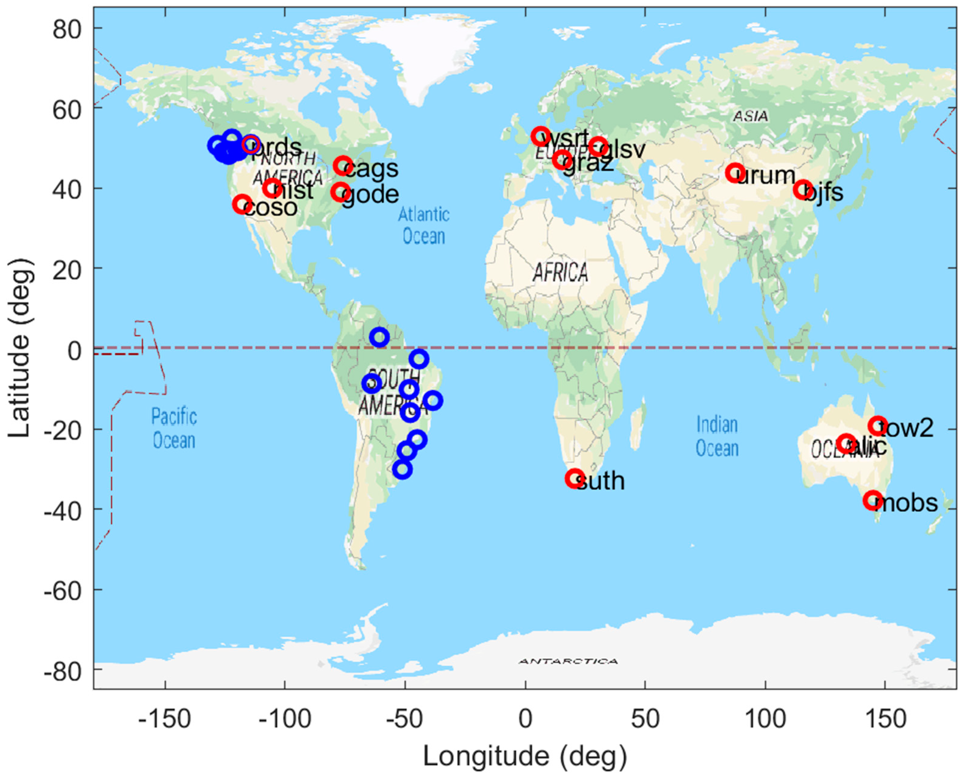
4.1. Data Description
4.2. IVH from the IRI 2016 Model
4.3. IVH Impacts on Mapping Errors
4.4. IVH Impacts on Ionospheric Modeling
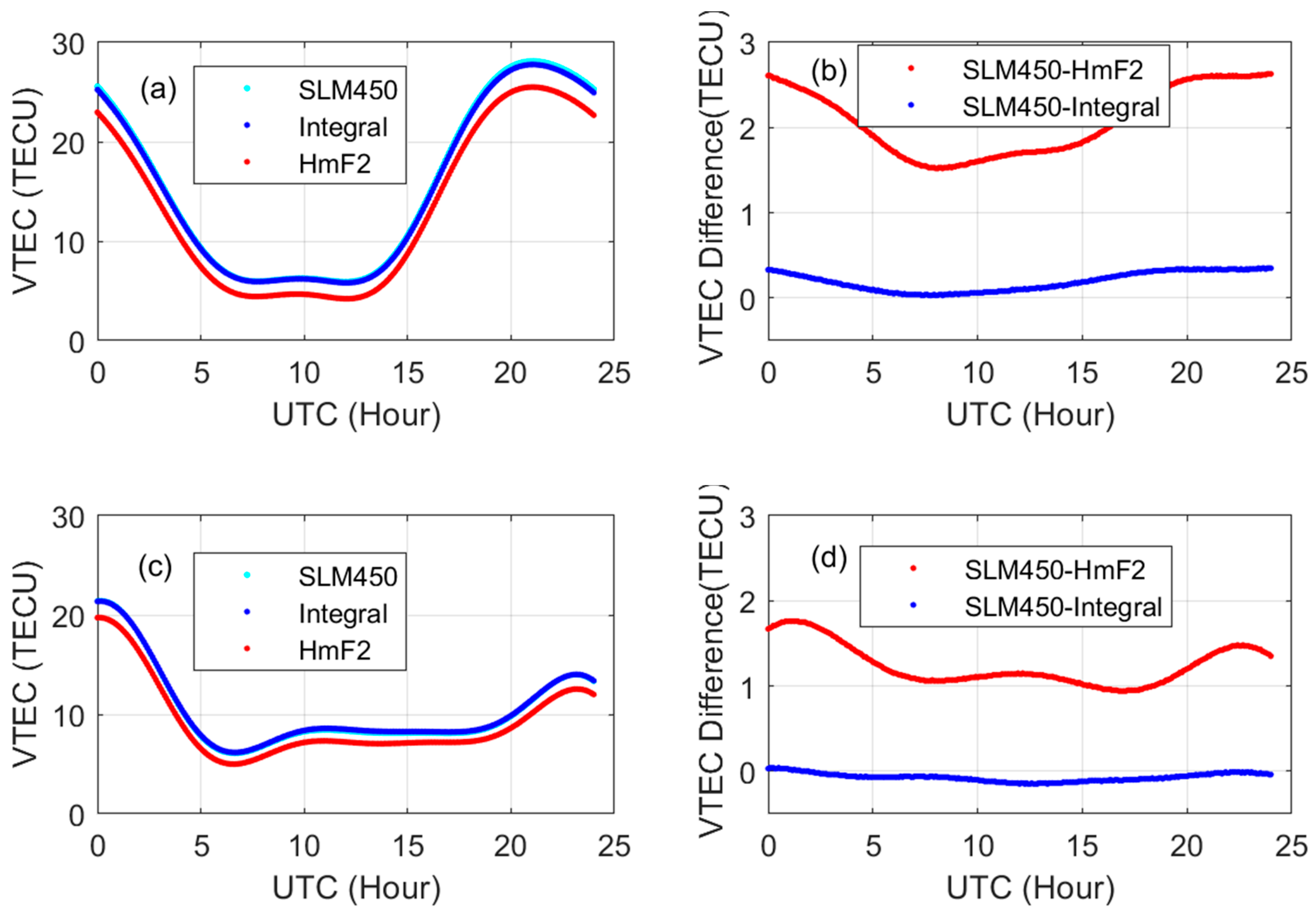
4.4.1. IVH Effects on VTEC
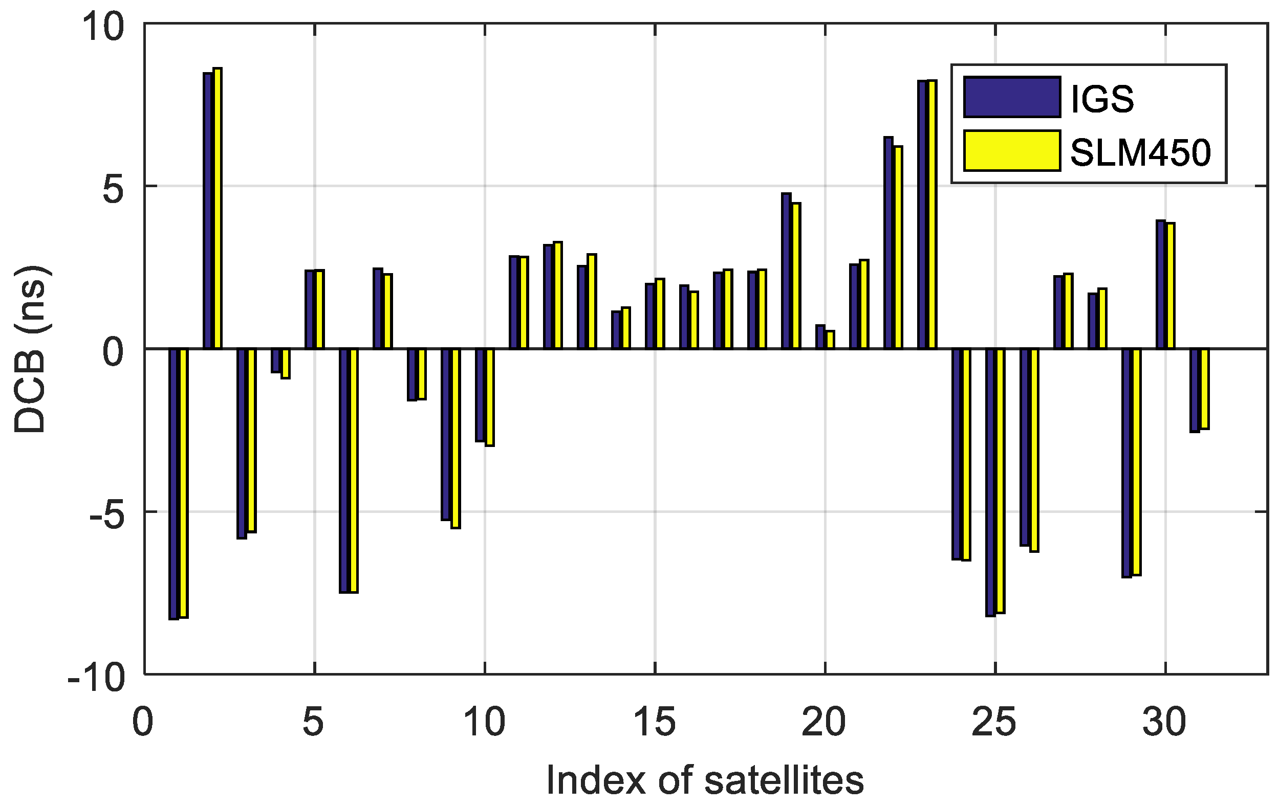
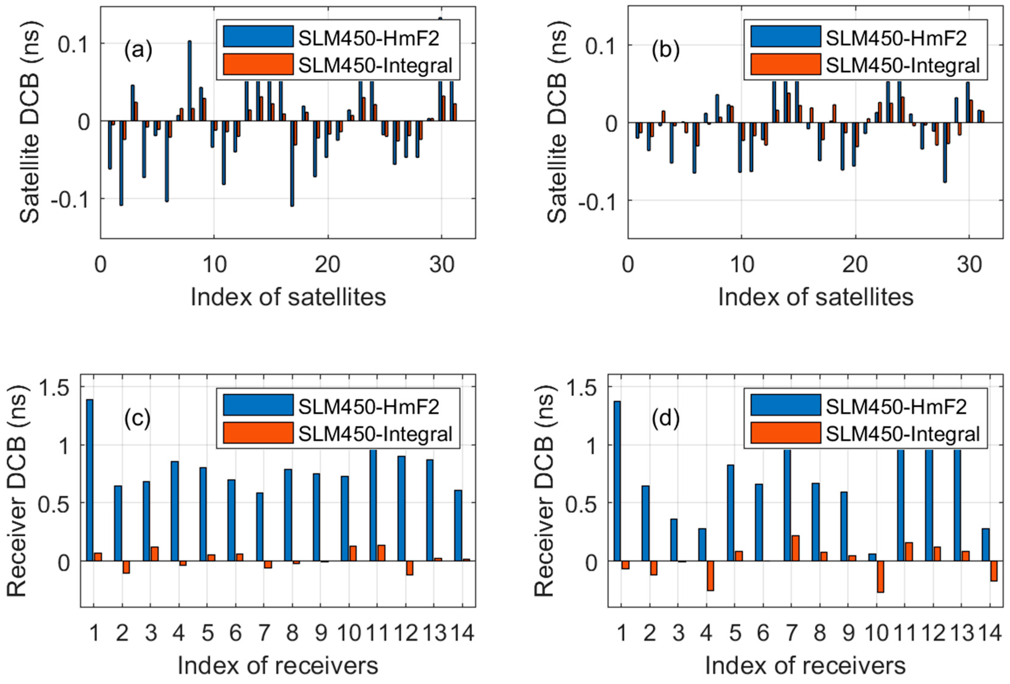
4.4.2. IVH Effects on Satellite and Receiver DCBs
5. Conclusions
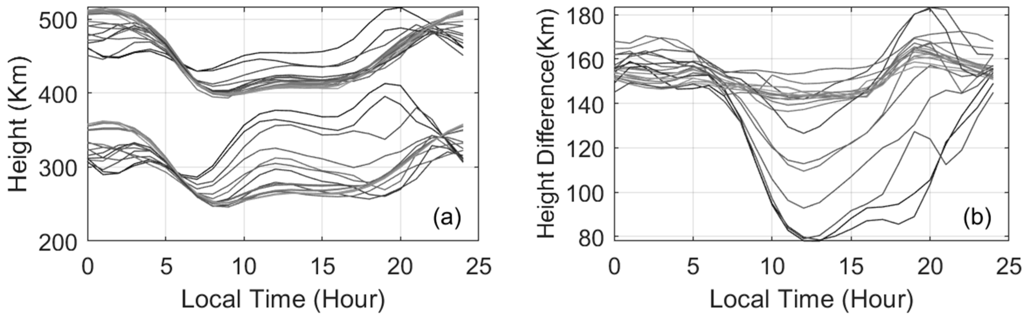
- (1)
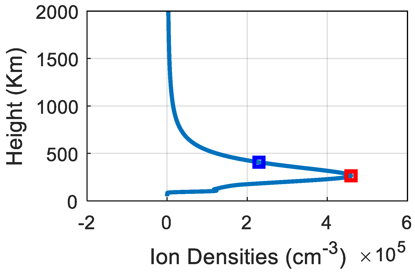
- The integral height and HmF2 varies about 100 km, with daytime lower, and nighttime higher. The height differences between the integral height and HmF2 were about 150 km.
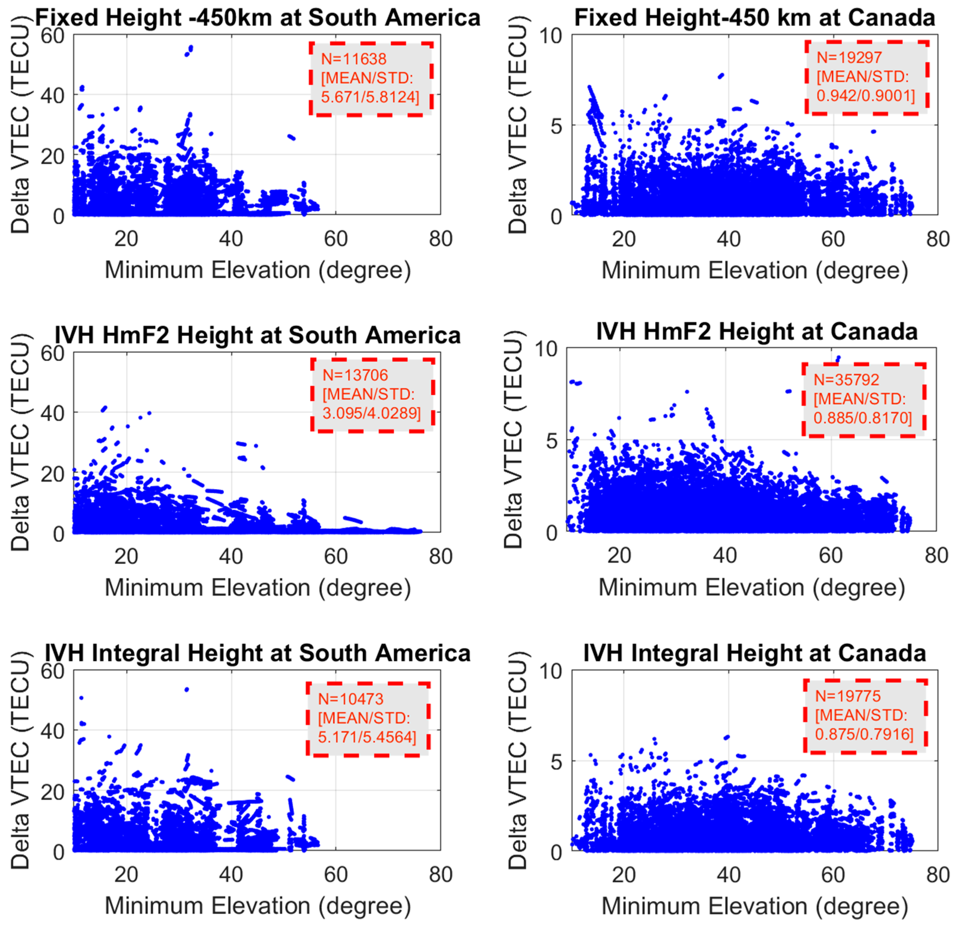
- (2)
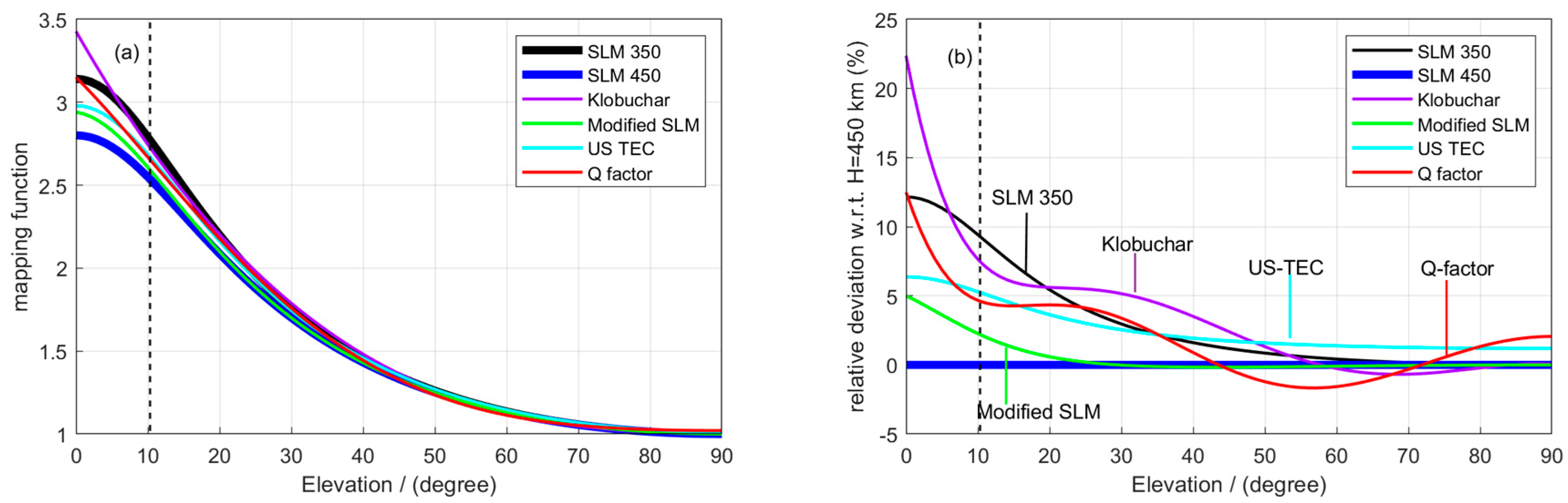
- Compared with using a fixed height of 450 km, the mapping errors using the integral height achieved an 8% reduction of mapping errors. Interestingly, 35% smaller mapping errors were found using HmF2 at the lower latitude.
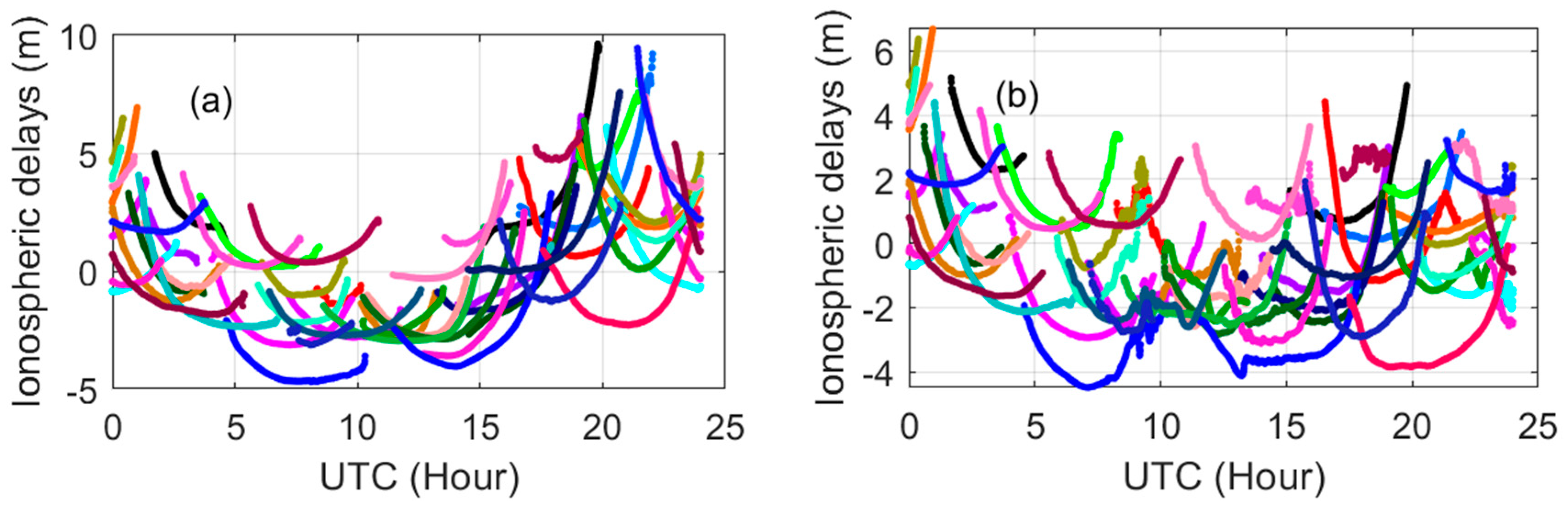
- (3)
- A higher height produces larger VTEC; lower height smaller VTEC. The modeled VTEC using HmF2 was up to 2.5 TECU smaller when compared with the VTEC using a fixed height of 450 km. By contrast, the difference of VTEC between the integral height and the fixed height was within 0.5 TECU.
- (4)
- The effects of IVH on the satellite DCBs using these three different heights was within 0.1 ns, and larger impact on receiver DCBs were at 1.0 ns. And the impact of HmF2 on receiver DCBs are all positive.
Author Contributions
Funding
Acknowledgments
Conflicts of Interest
References
- Mannucci, A.J.; Wilson, B.; Yuan, D. A global mapping technique for GPS-derived ionospheric total electron content measurements. Radio Sci. 1998, 33, 565–582. [Google Scholar] [CrossRef]
- Sardón, E.; Zarraoa, N. Estimation of total electron content using GPS data: How stable are the differential satellite and receiver instrumental biases? Radio Sci. 1997, 32, 1899–1910. [Google Scholar] [CrossRef]
- Li, Z.; Yuan, Y.; Li, H.; Ou, J.; Huo, X. Two-step method for the determination of the differential code biases of COMPASS satellites. J. Geod. 2012, 86, 1059–1076. [Google Scholar] [CrossRef]
- Nie, Z.; Zhou, P.; Liu, F.; Wang, Z.; Gao, Y. Evaluation of Orbit, Clock and Ionospheric Corrections from Five Currently Available SBAS L1 Services: Methodology and Analysis. Remote Sens. 2019, 11, 411. [Google Scholar] [CrossRef]
- Lanyi, G.E.; Roth, T. A comparison of mapped and measured total ionospheric electron content using global positioning system and beacon satellite observations. Radio Sci. 1988, 23, 483–492. [Google Scholar] [CrossRef]
- Hernández-Pajares, M.; Juan, J.; Sanz, J.; García-Fernández, M. Towards a More Realistic Ionospheric Mapping Function; XXVIII URSI General Assembly: Delhi, India, 2005. [Google Scholar]
- Brunini, C.; Camilion, E.; Azpilicueta, F. Simulation study of the influence of the ionospheric layer height in the thin layer ionospheric model. J. Geod. 2011, 85, 637–645. [Google Scholar] [CrossRef]
- Wang, X.-L.; Wan, Q.-T.; Ma, G.-Y.; Li, J.-H.; Fan, J.-T. The influence of ionospheric thin shell height on TEC retrieval from GPS observation. Res. Astron. Astrophys. 2016, 16, 116. [Google Scholar] [CrossRef]
- Birch, M.J.; Hargreaves, J.K.; Bailey, G.J. On the use of an effective ionospheric height in electron content measurement by GPS reception. Radio Sci. 2002, 37. [Google Scholar] [CrossRef]
- Nava, B.; Radicella, S.M.; Leitinger, R.; Coïsson, P. Use of total electron content data to analyze ionosphere electron density gradients. Adv. Space Res. 2007, 39, 1292–1297. [Google Scholar] [CrossRef]
- Zhao, J.; Zhou, C. On the optimal height of ionospheric shell for single-site TEC estimation. GPS Solut. 2018, 22, 48. [Google Scholar] [CrossRef]
- Hernandez-Pajares, M.; Juan, J.M.; Sanz, J.; Orus, R.; Garcia-Rigo, A.; Feltens, J.; Komjathy, A.; Schaer, S.C.; Krankowski, A. The IGS VTEC maps: A reliable source of ionospheric information since 1998. J. Geod. 2009, 83, 263–275. [Google Scholar] [CrossRef]
- Leitinger, R.; Spalla, P.; Ciraolo, L. Latitude Dependent Mean Ionospheric Height—A New Approach to the TEC Evaluation from NNSS Data. Acta Geod. Geophys. Hung. 1998, 33, 61–73. [Google Scholar] [CrossRef]
- Mushini, S.C.; Jayachandran, P.T.; Langley, R.B.; MacDougall, J.W. Use of varying shell heights derived from ionosonde data in calculating vertical total electron content (TEC) using GPS—New method. Adv. Space Res. 2009, 44, 1309–1313. [Google Scholar] [CrossRef]
- Komjathy, A.; Langley, R. The effect of shell height on high precision ionospheric modelling using GPS. In Proceedings of the 1996 IGS Workshop International GPS Service for Geodynamics (IGS), Silver Spring, MD, USA, 19–21 March 1996. [Google Scholar]
- Zhang, B.; Ou, J.; Yuan, Y.; Li, Z. Extraction of line-of-sight ionospheric observables from GPS data using precise point positioning. Sci. China Earth Sci. 2012, 55, 1919–1928. [Google Scholar] [CrossRef]
- Xiang, Y.; Gao, Y.; Shi, J.; Xu, C. Consistency and analysis of ionospheric observables obtained from three precise point positioning models. J. Geod. 2019, 2019, 1–10. [Google Scholar] [CrossRef]
- Klobuchar, J.A. Ionospheric time-delay algorithm for single-frequency GPS users. IEEE Trans. Aerosp. Electron. Syst. AES 1987, 23, 325–331. [Google Scholar] [CrossRef]
- Schaer, S. Mapping and Predicting the Earth’s Ionosphere Using the Global Positioning System. Ph.D. Thesis, University of Berne, Bern, Switzerland, 1999. [Google Scholar]
- Coster, A.J.; Gaposchkin, E.M.; Thornton, L.E. Real-Time Ionospheric Monitoring System Using GPS. Navigation 1992, 39, 191–204. [Google Scholar] [CrossRef]
- Smith, D.A.; Araujo-Pradere, E.A.; Minter, C.; Fuller-Rowell, T. A comprehensive evaluation of the errors inherent in the use of a two-dimensional shell for modeling the ionosphere. Radio Sci. 2008, 43, 1–23. [Google Scholar] [CrossRef]
- Clynch, J.R.; Coco, D.S.; Coker, C.; Bishop, G.J. A versatile GPS ionospheric monitor-High latitude measurements of TEC and scintillation. In Proceedings of the Institute of Navigation Satellite Division, 2nd International Technical Meeting, Colorado Springs, CO, USA, 27–29 September 1989; pp. 445–450. [Google Scholar]
- Wen, J.; Wan, W.; Ding, F.; Yue, X.; She, C.; Liu, L. Experimental observation and statistical analysis of the vertical TEC mapping function. Chin. J. Geophys. 2018, 53, 22–29. [Google Scholar]
- Conker, R.S.; El-Arini, M.B. An ionospheric obliquity process responsive to line-of-sight azimuth and elevation. Radio Sci. 2002, 37, 1097. [Google Scholar] [CrossRef]
- Zhong, J.; Lei, J.; Dou, X.; Yue, X. Assessment of vertical TEC mapping functions for space-based GNSS observations. GPS Solut. 2016, 20, 353–362. [Google Scholar] [CrossRef]
- Niranjan, K.; Srivani, B.; Gopikrishna, S.; Rama Rao, P. Spatial distribution of ionization in the equatorial and low-latitude ionosphere of the Indian sector and its effect on the pierce point altitude for GPS applications during low solar activity periods. J. Geophys. Res. Space Phys. 2007, 112. [Google Scholar] [CrossRef]
- Li, M.; Yuan, Y.; Zhang, B.; Wang, N.; Li, Z.; Liu, X.; Zhang, X. Determination of the optimized single-layer ionospheric height for electron content measurements over China. J. Geod. 2018, 92. [Google Scholar] [CrossRef]
- Radicella, S.M.; Nava, B.; Coïsson, P.; Kersley, L.; Bailey, G.J. Effects of gradients of the electron density on Earth-space communications. Ann. Geophys. 2004, 47. [Google Scholar] [CrossRef]
- Komjathy, A.; Sparks, L.; Mannucci, A.J.; Coster, A. The ionospheric impact of the October 2003 storm event on Wide Area Augmentation System. GPS Solut. 2005, 9, 41–50. [Google Scholar] [CrossRef]
- Yuan, Y.; Ou, J. A generalized trigonometric series function model for determining ionospheric delay. Prog. Nat. Sci. 2004, 14, 1010–1014. [Google Scholar] [CrossRef]
- WDC. World Data Center for Geomagnetism. Available online: http://wdc.kugi.kyoto-u.ac.jp/dstdir/ (accessed on 19 November 2017).
- Xiang, Y.; Gao, Y. Improving DCB Estimation Using Uncombined PPP. Navigation 2017, 64, 463–473. [Google Scholar] [CrossRef]
- Memarzadeh, Y. Ionospheric Modeling for Precise GNSS Applications. Ph.D. Thesis, Technische Universiteit Delft, Delft, The Netherlands, 2009. [Google Scholar]


| Strategies | Ionospheric Modeling |
|---|---|
| Ionospheric model function at a station | General Triangle Series Function (GTSF) |
| Elevation cut-off | 20° |
| Coordinate frame | Geographic frame |
| Height | Ionospheric varying height (IVH) from the IRI 2016 model |
| Satellite and receiver DCB separation | Zero-mean reference of all available satellites |
| Assumptions | The ionospheric electron content is condensed in an infinitesimal thickness layer, and an MF converts the slant total electron content (STEC) into the vertical total electron content (VTEC) The biases are assumed to be a constant during a day. |
© 2019 by the authors. Licensee MDPI, Basel, Switzerland. This article is an open access article distributed under the terms and conditions of the Creative Commons Attribution (CC BY) license (http://creativecommons.org/licenses/by/4.0/).
Share and Cite
Xiang, Y.; Gao, Y. An Enhanced Mapping Function with Ionospheric Varying Height. Remote Sens. 2019, 11, 1497. https://doi.org/10.3390/rs11121497
Xiang Y, Gao Y. An Enhanced Mapping Function with Ionospheric Varying Height. Remote Sensing. 2019; 11(12):1497. https://doi.org/10.3390/rs11121497
Chicago/Turabian StyleXiang, Yan, and Yang Gao. 2019. "An Enhanced Mapping Function with Ionospheric Varying Height" Remote Sensing 11, no. 12: 1497. https://doi.org/10.3390/rs11121497
APA StyleXiang, Y., & Gao, Y. (2019). An Enhanced Mapping Function with Ionospheric Varying Height. Remote Sensing, 11(12), 1497. https://doi.org/10.3390/rs11121497