Night Thermal Unmixing for the Study of Microscale Surface Urban Heat Islands with TRISHNA-Like Data

Abstract

Urban Heat Islands (UHIs) at the surface and canopy levels are major issues in urban planification and development. For this reason, the comprehension and quantification of the influence that the different land-uses/land-covers have on UHIs is of particular importance. In order to perform a detailed thermal characterisation of the city, measures covering the whole scenario (city and surroundings) and with a recurrent revisit are needed. In addition, a resolution of tens of meters is needed to characterise the urban heterogeneities. Spaceborne remote sensing meets the first and the second requirements but the Land Surface Temperature (LST) resolutions remain too rough compared to the urban object scale. Thermal unmixing techniques have been developed in recent years, allowing LST images during day at the desired scales. However, while LST gives information of surface urban heat islands (SUHIs), canopy UHIs and SUHIs are more correlated during the night, hence the development of thermal unmixing methods for night LSTs is necessary. This article proposes to adapt four empirical unmixing methods of the literature, Disaggregation of radiometric surface Temperature (DisTrad), High-resolution Urban Thermal Sharpener (HUTS), Area-To-Point Regression Kriging (ATPRK), and Adaptive Area-To-Point Regression Kriging (AATPRK), to unmix night LSTs. These methods are based on given relationships between LST and reflective indices, and on invariance hypotheses of these relationships across resolutions. Then, a comparative study of the performances of the different techniques is carried out on TRISHNA synthesized images of Madrid. Since TRISHNA is a mission in preparation, the synthesis of the images has been done according to the planned specification of the satellite and from initial Aircraft Hyperspectral Scanner (AHS) data of the city obtained during the DESIREX 2008 capaign. Thus, the coarse initial resolution is 60 m and the finer post-unmixing one is 20 m. In this article, we show that: (1) AATPRK is the most performant unmixing technique when applied on night LST, with the other three techniques being undesirable for night applications at TRISHNA resolutions. This can be explained by the local application of AATPRK. (2) ATPRK and DisTrad do not improve significantly the LST image resolution. (3) HUTS, which depends on albedo measures, misestimates the LST, leading to the worst temperature unmixing. (4) The two main factors explaining the obtained performances are the local/global application of the method and the reflective indices used in the LST-index relationship.

1. Introduction

Canopy Urban Heat Islands (UHIs), defined as the higher air temperatures of urban areas compared to surrounding countryside [1], have been shown to influence human health [2,3], to affect urban air pollution [4], and to alter the energy consumption needs [5,6]. Therefore, understanding the urban parameters impacting canopy UHIs formation and the dynamics behind their development appears as crucial to enhance urban well-being. In the last years, several works shown that land-use characteristics such as building density, surface materials, presence of green areas, or sky view factors influence canopy UHI development [7,8].

Air temperature data covering a large spatial area and with a high revisit time are unusual due to the locality (in space or in time) of the measures [9,10]. On the other hand, spaceborne remote sensing can cover the city together with rural areas around, it presents revisit times from some days to some weeks, and it allows to measure Land Surface Temperatures (LSTs) by using the Thermal InfraRed (TIR) bands of the sensors. Furthermore, these LSTs can be used to estimate Surface Urban Heat Islands (SUHIs). These SUHIs are defined as the higher surface temperatures in urban areas than in surrounding rural ones [11,12]. It has been shown that SUHI should be measured during the night to be informative on the urban heat islands at canopy level [12], since surface and canopy heat islands are more decorrelated during day.

Both canopy UHIs and SUHIs deliver global information of the city temperature compared to the rural area around. However, urban thermal environment is not homogeneous, and then intra-urban temperature differences appear due to differences in the land-use/land cover. Several projects are currently under study to develop thermal satellites with high enough spatial resolution and revisit capacities to characterize the microscale structure of SUHIs. These are the Indian (ISRO)-French (CNES) mission TRISHNA [13], the European (ESA) LSTM [14], and HyspIRI in NASA/JPL [15]. But such missions lack in their spatial resolution of about 50–60 m and are not able to discern the local LST on an urban object scale. Since to characterize the urban thermal structure resolutions of around ten meters allowing to discriminate the urban fabric (street net) are necessary [16], thermal unmixing techniques have been developed.

Thermal unmixing techniques based on empirical relationships between LST and reflective domain indices allow for low resoluted LST images to reach the high resolution of the reflective domain [17]. In the last decades, several empirical techniques were developed [18,19,20,21]. Unfortunately, reflective information is not available during the night and alternatives should be found. For the moment, few works present alternatives to unmix night LST and these alternatives should be studied more carefully: Wicki et al., 2017 propose to use land use/land cover maps of urban environments as high resoluted information to use in the LST-indices relationship [22] (but they do not study the performance of this possible unmixing alternative for night) and Ribeiro-Pereira et al. 2018 use day Near InfraRed (NIR) and Short Wave InfraRed (SWIR) bands as high resoluted (90 m) information to unmix night LST (initially resoluted at 540 m) in a rural scenario [23] (without analyzing the possible effects of using day reflectif information for night unmixing).

The main goal of this article is to study the potentiality, to characterize microscale SUHIs, of night LST unmixing using day reflective indices as high resoluted information. With this purpose, the performances of four thermal unmixing methods—Disaggregation of radiometric surface Temperature (DisTrad) [18,24], High-resolution Urban Thermal Sharpener (HUTS) [19], Area-To-Point Regression Kriging (ATPRK) [25], and Adaptive Area-To-Point Regression Kriging (AATPRK) [20]—have been studied when unmixing night LSTs of an urban scenario. To do so, TRISHNA satellite images have been synthesized by correcting and aggregating Aircraft Hyperspectral Scanner (AHS) images of Madrid obtained during the DESIREX 2008 campaign. At present, TRISHNA is a mission in preparation whose specifications are still being defined. So, synthetic TRISHNA images according to the planned configuration in both reflectif and thermal domains are used to study SUHI and microscale SUHIs characterizing the heterogeneity of the urban fabric.

In Section 2, the AHS data from DESIREX 2008 campaign is presented, as well as the synthesis of TRISHNA images from airborne data. Section 3 contains the methodology used to study SUHI and microscale SUHIs. It contains 4 subsections: in Section 3.1 the used unmixing methods are explained together with the hypotheses on which they ground, in Section 3.2 the adaptation of these techniques to unmix night-LST is explained, in Section 3.3 the SUHI estimation is described, and in Section 3.4 the evaluation criteria used to characterize the unmixing performances are presented. In Section 4, the night LST unmixing results are shown: firstly in Section 4.1 the relationship between night LST and day reflective indices is studied, and secondly in Section 4.2 the night unmixing performances of the different methods are compared and SUHI and microscale SUHIs are characterized. Finally, in Section 5 the conclusions and perspectives of this work are presented.

2. Datasets

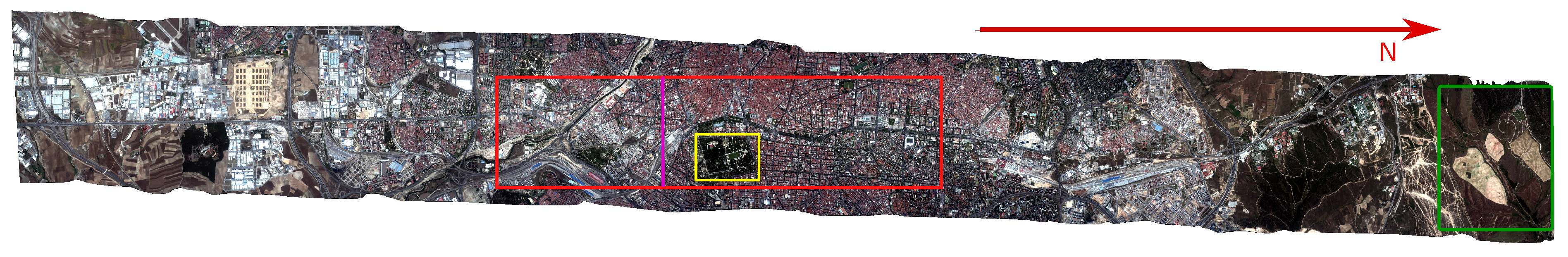
2.1. DESIREX Dataset

Airborne Hyperspectral Scanner (AHS) data acquired over the city of Madrid, during the DESIREX campaign 2008 [12,26,27,28] (summer), at 4 m resolution over 80 spectral channels (0.443–13.4 $\mathsf{\mu }$m) is used. The exact analyzed data correspond to six (three day and three night) urban and suburban images of Madrid from Getafe to Universidad Autónoma obtained at 2497 m altitude, see Figure 1. The flight lines were performed: the 28 June at 11:53 for the day image and at 21:44 for the night one, the 1 July at 11:44 for day and at 22:12 for night, and the 4 July at 11:32 and 22:14 for day and night images respectively. For each date, the day and night images are all registered.

Together with these aircraft hyperspectral images, atmospheric characterizations were performed each day. Temperature profiles and atmospheric water vapour amount were measured with soundings from ground level to 25 km altitude. In addition, relative humidity and air temperature were also measured in fixed masts. These measures were performed several times a day and at different emplacements. The complete description of the dataset can be found in the DESIREX 2008 final report [12,26,27,28].

2.2. Multispectral Satellite Modelling

This paper focuses on the study of SUHIs with TRISHNA-like [13] multispectral satellite. Satellite radiance images are modelled from AHS radiance acquisitions using direct and inverse radiative transfer tools COCHISE and COMANCHE [29] and next applying a spatial aggregation to reach TRISHNA resolutions. From the hyperspectral images at 4 m resolution, the images obtained by TRISHNA, with 60 m resolution in the TIR bands and 20 m resolution in the reflective bands, are synthesized. The modelled TRISHNA satellite counts with four bands in the Visible and Near InfraRed (VNIR) domain, one band in the SWIR and four bands in the TIR domain. The used AHS bands are those closer to the planned set-up of the future French–Indian mission TRISHNA, see

Table 1. Planned spectral and spatial characterization of TRISHNA multispectral satellite.

TRISHNA Band	Wavelength Center	FWHM	Resolution
Band 1-Blue	485 nm	70 nm	20 m
Band 2-Green	555 nm	70 nm
Band 3-Red	670 nm	60 nm
Band 4-NIR	860 nm	40 nm
Band 5-SWIR	1610 nm	150 nm
Band 6-TIR 1	8660 nm	390 nm	60 m
Band 7-TIR 2	9150 nm	410 nm
Band 8-TIR 3	10,590 nm	550 nm
Band 9-TIR 4	11,780 nm	560 nm

.

The preprocessing from the initial AHS radiance at the aircraft level to the final Top Of Atmosphere (TOA) radiance images depends on the spectral domain, being different for the reflective and for the thermal bands [21]. However, the spatial aggregation procedure, which depends on the Signal to Noise Ratio (SNR) and the Modulation Transfert Function (MTF), is the same for reflective and thermal ranges [21]. The SNR and the MTF have been chosen for each spectral range according to the TRISHNA specifications. Once the TRISHNA TOA radiance images have been synthesized, they are corrected to obtain the Bottom Of Atmosphere (BOA) reflectance in the VNIR-SWIR domain [29], and the BOA radiance in the TIR domain. A detailed description of the synthesis of the satellite images is available in Granero-Belinchon et al., 2019 [21].

3. Methodology

From BOA day reflectance images, indices characterizing the ground-use are estimated at 20 m resolution. Day reflectance images are also aggregated to 60 m resolution and indices are newly estimated (green steps of Figure 2). The reflective indices used along this article are Normalized Difference Vegetation index (NDVI) [30], Normalized Difference Built-Up Index (NDBI) [30], and albedo (estimated following [26]). Concurrently, from BOA TIR night radiances, LST at 60 m resolution is estimated using Temperature and Emissivity Separation (TES) [31] (red steps of Figure 2). Inside the TES algorithm, the band used to get the LST is the band with the highest emissivity. Next, thermal unmixing methods based on night-LST vs. day-Index regressions at 60 m resolution are applied to estimate the new night-LST at 20 m resolution (orange steps of Figure 2). Finally, SUHIs are studied by subtracting to the city center LST the averaged near countryside LST (blue steps of Figure 2).

3.1. Thermal Unmixing Techniques

In this article, four empirical thermal unmixing techniques are studied: DisTrad [24,32,33], HUTS [19], ATPRK [20,25], and AATPRK [20]. These unmixing procedures rely on the basis that reflective domain images are acquired at a better resolution than TIR domain ones, and consequently, the higher resolution information obtained in the reflective domain can be used to unmix the TIR images. These empirical methods express the LST as a function of a given reflective index at the coarse TIR resolution (L):

$$T_L=f_L\left(I_L\right)$$

(1)

A regression is then performed at this resolution to obtain the parameters defining the function $f_L$. Supposing that $f_L$ is invariant across resolutions ($f_L=f$) and using the reflective index at the fine resolution $\eta$, it is possible to approximate the LST at this fine resolution (${\widehat{T}}_{\eta }$):

$${\widehat{T}}_{\eta }=f\left(I_{\eta }\right)$$

(2)

At this stage, the fine resolution LST is approximated by the strict function $f\left(I_{\eta }\right)$. To take into account spatial disagreements with the strict behaviour of the function, a residual correction of the unmixed LST is performed to estimate the fine resolution LST, $T_{\eta }$ [21]. This residual correction is different and relies on different hypotheses depending on the unmixing technique [21].

Thus, the fundamental hypotheses of these procedures are:

• First, LST behaves as a function of a given reflective index at the coarse resolution L. Depending on the technique, this relationship is linear for DisTrad and ATPRK, Equation (3), locally linear for AATPRK, Equation (4), or fourth order polynomial for HUTS, Equation (5). A regression at this resolution allows to obtain the parameters characterizing the behavior of LST versus index.

  $$\begin{array}{ccc}\hfill T_L\left(x_L\right)=& a+b{I}_L\left(x_L\right)\hfill & \hfill \mathrm{DisTrad}\mathrm{and}\mathrm{ATPRK}\end{array}$$

  (3)

  $$\begin{array}{ccc}\hfill T_L\left(x_L\right)=& a\left(x_{L,0}\right)+b\left(x_{L,0}\right)I_L\left(x_L\right)\forall x_L\in N\hfill & \hfill \mathrm{AATPRK}\end{array}$$

  (4)

  $$\begin{array}{ccc}\hfill T_L\left(x_L\right)=& p_1{I}_L{\left(x_L\right)}^4+p_2{I}_L{\left(x_L\right)}^3{\alpha }_L\left(x_L\right)+p_3{I}_L{\left(x_L\right)}^2{\alpha }_L{\left(x_L\right)}^2+\hfill & \hfill \mathrm{HUTS}\end{array}$$

  (5)

  $$\begin{array}{c}+p_4{I}_L\left(x_L\right){\alpha }_L{\left(x_L\right)}^3+p_5{\alpha }_L{\left(x_L\right)}^4+p_6{I}_L{\left(x_L\right)}^3+\hfill \\ +p_7{I}_L{\left(x_L\right)}^2{\alpha }_L\left(x_L\right)+p_8{I}_L\left(x_L\right){\alpha }_L{\left(x_L\right)}^2+p_9{\alpha }_L{\left(x_L\right)}^3+\hfill \\ +p_{10}{I}_L{\left(x_L\right)}^2+p_{11}{I}_L\left(x_L\right){\alpha }_L\left(x_L\right)+p_{12}{\alpha }_L{\left(x_L\right)}^2\hfill \\ +p_{13}{I}_L\left(x_L\right)+p_{14}{\alpha }_L\left(x_L\right)+p_{15}\hfill \end{array}$$

  where both LST and indices depend on the pixel location x ($x_L$ and $x_{\eta }$ for coarse and fine resolutions respectively). a and b are the intercept and slope obtained in the regression with DisTrad and ATPRK. $a\left(x_{L,0}\right)$ and $b\left(x_{L,0}\right)$ are the local intercept and slope obtained for coarse pixel $x_{L,0}$ by performing the regression with the N coarse pixels around [20]. Parameters $p_i$ are those obtained in the polynomial regression.
• Second, the behavior of the LST in function of the index and the regression parameters defining this behavior are scale invariant. Therefore, they can be used together with the measured index at the fine scale $\eta$ to estimate the LST at this resolution, Equation (6) for DisTrad and ATPRK, Equation (7) for AATPRK, and Equation (8) for HUTS.

  $$\begin{array}{ccc}\hfill {\widehat{T}}_{\eta }\left(x_{\eta }\right)=& a+b{I}_{\eta }\left(x_{\eta }\right)\hfill & \hfill \mathrm{DisTrad}\mathrm{and}\mathrm{ATPRK}\end{array}$$

  (6)

  $$\begin{array}{ccc}\hfill {\widehat{T}}_{\eta }\left(x_{\eta }\right)=& a\left(x_{L,0}\right)+b\left(x_{L,0}\right)I_{\eta }\left(x_{\eta }\right)\forall x_{\eta }\in x_{L,0}\hfill & \hfill \mathrm{AATPRK}\end{array}$$

  (7)

  $$\begin{array}{ccc}\hfill {\widehat{T}}_{\eta }\left(x_{\eta }\right)=& p_1{I}_{\eta }{\left(x_{\eta }\right)}^4+p_2{I}_{\eta }{\left(x_{\eta }\right)}^3{\alpha }_{\eta }\left(x_{\eta }\right)+p_3{I}_{\eta }{\left(x_{\eta }\right)}^2{\alpha }_{\eta }{\left(x_{\eta }\right)}^2+\hfill & \hfill \mathrm{HUTS}\end{array}$$

  (8)

  $$\begin{array}{c}+p_4{I}_{\eta }\left(x_{\eta }\right){\alpha }_{\eta }{\left(x_{\eta }\right)}^3+p_5{\alpha }_{\eta }{\left(x_{\eta }\right)}^4+p_6{I}_{\eta }{\left(x_{\eta }\right)}^3+\hfill \\ +p_7{I}_{\eta }{\left(x_{\eta }\right)}^2{\alpha }_{\eta }\left(x_{\eta }\right)+p_8{I}_{\eta }\left(x_{\eta }\right){\alpha }_{\eta }{\left(x_{\eta }\right)}^2+p_9{\alpha }_{\eta }{\left(x_{\eta }\right)}^3+\hfill \\ +p_{10}{I}_{\eta }{\left(x_{\eta }\right)}^2+p_{11}{I}_{\eta }\left(x_{\eta }\right){\alpha }_{\eta }\left(x_{\eta }\right)+p_{12}{\alpha }_{\eta }{\left(x_{\eta }\right)}^2\hfill \\ +p_{13}{I}_{\eta }\left(x_{\eta }\right)+p_{14}{\alpha }_{\eta }\left(x_{\eta }\right)+p_{15}\hfill \end{array}$$
• Third, the residuals estimation of the fine resolution LST are also based on an scale invariance. DisTrad residuals correction supposes that the coarse resolution residuals are equal to the fine resolution ones, Equation (9). ATPRK and AATPRK present a more complex estimation of the fine scale residuals based on a weighted linear combination of surrounding coarse scale residuals, Equation (10). The weights of this method are those optimizing the estimator: the bias has to be zero and the variance has to be minimal [20,25]. Finally, HUTS links the pixel LST reconstruction error to the fine residual, Equation (11).

  $$\begin{array}{ccc}\hfill \Delta T_{\eta }\left(x_{\eta }\right)=& \Delta T_L\left(x_L\right)=T_L\left(x_L\right)-(a+b{I}_L\left(x_L\right))\forall x_{\eta }\in x_L\hfill & \hfill \mathrm{DisTrad}\end{array}$$

  (9)

  $$\begin{array}{ccc}\hfill \Delta T_{\eta }\left(x_{\eta }\right)=& \sum _{i+1}^N{\lambda }_i\Delta T_L\left(x_{L,i}\right)\hfill & \hfill \mathrm{ATPRK}\mathrm{and}\mathrm{AATPRK}\end{array}$$

  (10)

  $$\begin{array}{ccc}\hfill \Delta T_{\eta }\left(x_{\eta }\right)=& \Delta T_L\left(x_L\right)=T_L\left(x_L\right)-\frac{1}{N_{\eta }}\sum _{x_{\eta }\in x_L}{\widehat{T}}_{\eta }\left(x_{\eta }\right)\forall x_{\eta }\in x_L\hfill & \hfill \mathrm{HUTS}\end{array}$$

  (11)

  where ${\lambda }_i$ of Equation (10) are the weights of the surrounding coarse pixels $x_{L,i}$ used in the estimation of the fine residual. In Equation (11), $N_{\eta }$ is the number of fine pixels within a coarse one.

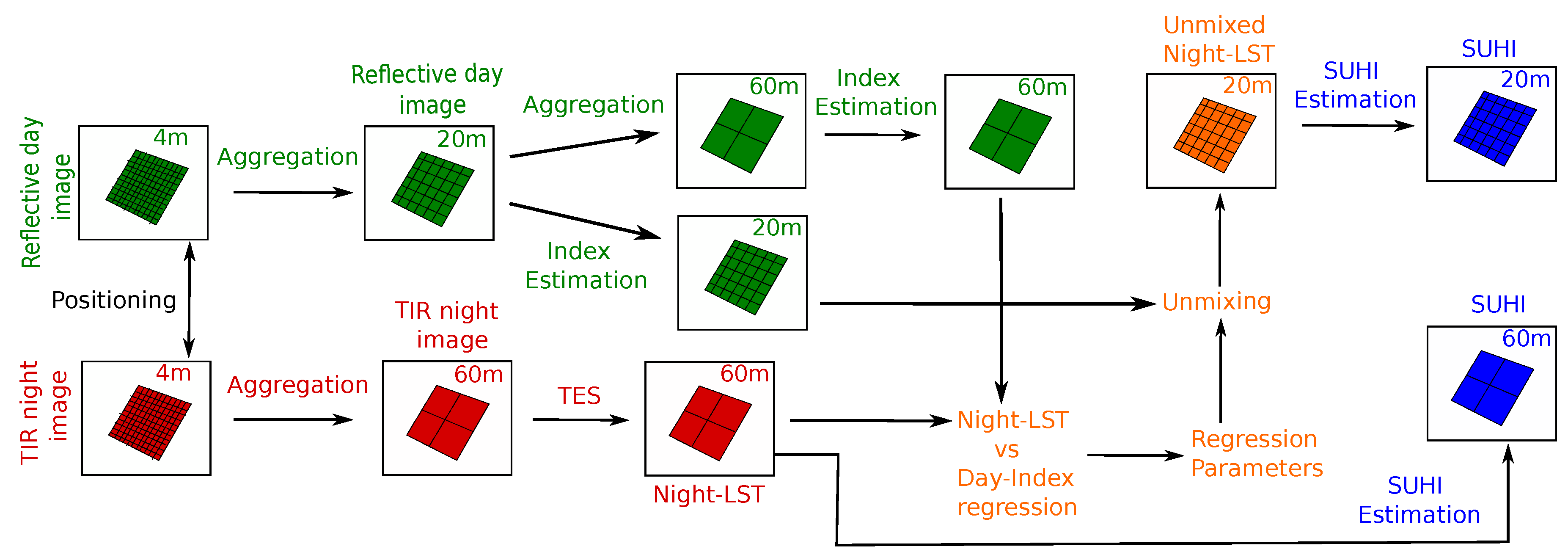
The final unmixed LSTs are expressed as:

$$T_{\eta }\left(x_{\eta }\right)={\widehat{T}}_{\eta }\left(x_{\eta }\right)+\Delta T_{\eta }\left(x_{\eta }\right)$$

(12)

3.2. Night Unmixing

All the unmixing techniques used in this article have shown very good performances on day LST unmixing [21]. However, night reflective images are non-informative and they can not be used to unmix night LSTs. Surface Urban Heat Islands should be studied during the night to be informative on the heat island at surface and canopy level [12,34]. So, in this paper, the use of empirical unmixing techniques with the reflective indices obtained during day and the LST measured on night is proposed to study the thermal heterogeneities of Madrid during the night. Thus, at the coarse resolution L:

$$T_{L,night}=f_L\left(I_{L,day}\right)$$

(13)

A regression is performed to obtain the parameters defining $f_L$. This function is hypothesized to be the same at the fine scale $\eta$ ($f_L=f_{\eta }=f$). Then, the unmixed night LST can be approximated as:

$${\widehat{T}}_{\eta ,night}=f\left(I_{\eta ,day}\right)$$

(14)

As for day LST unmixing, a residuals correction is finally performed. The LST-index regression, the residuals estimation, and their hypotheses depend on the unmixing technique [21], see Equations (3)–(11).

Thus, night LST unmixing is based on the hypothesis that night LST behaves as a function f of selected day reflective indices. The scale invariance hypotheses of day LST unmixing are directly extrapolated to the night case.

3.3. SUHI and Microscale SUHI Estimation

For each night LST image, either measured or unmixed (see Figure 2), microscale SUHIs are estimated by subtracting to the LST of Madrid city center (red rectangle region in Figure 1) the averaged LST measured in the near countryside (green rectangle region in Figure 1). As LST, microscale SUHI depends on the pixel location x:

$$\mathcal{S}\left(x\right)=T_{\mathrm{urban}}\left(x\right)-〈T_{\mathrm{rural}}\left(x\right)〉$$

(15)

On the other hand, SUHI estimated as the mean value of microscale SUHI is also calculated [11]:

$$〈\mathcal{S}\left(x\right)〉=〈T_{\mathrm{urban}}\left(x\right)〉-〈T_{\mathrm{rural}}\left(x\right)〉$$

(16)

In this work, it has been decided to associate the urban environment with the city center of Madrid (red rectangle in Figure 1), while for the rural area, it has been decided to use a heterogeneous countryside land far enough from the city (green rectangle in Figure 1). These choices allow to avoid possible border effects.

3.4. Evaluation Criteria

The performance of each thermal unmixing methodology on night LSTs is characterized in order to conclude wheter these techniques can be used or not to study microscale SUHIs. Night land surface temperature calculated at 20 m resolution is used as reference along the article. To obtain this LST at 20 m, TES is applied on atmospherically corrected radiances at 20 m aggregated from 4 m AHS data. Then, to compare the performances of the different unmixing techniques, root mean square error (RMSE), mean bias error (MBE), and cross correlation (R) between reference and unmixed LSTs are estimated. These three quantitites are global criteria. Finally, the Structural Similarity Index (SSIM) [35], which is a local criterion, is also computed for each case.

4. Results and Discussion

In this section, only the results obtained for the 28 June are shown. However, unmixed night-LSTs have also been studied for DESIREX 2008 data from the 1 July and the 4 July, leading to equivalent conclusions, see Appendix A.

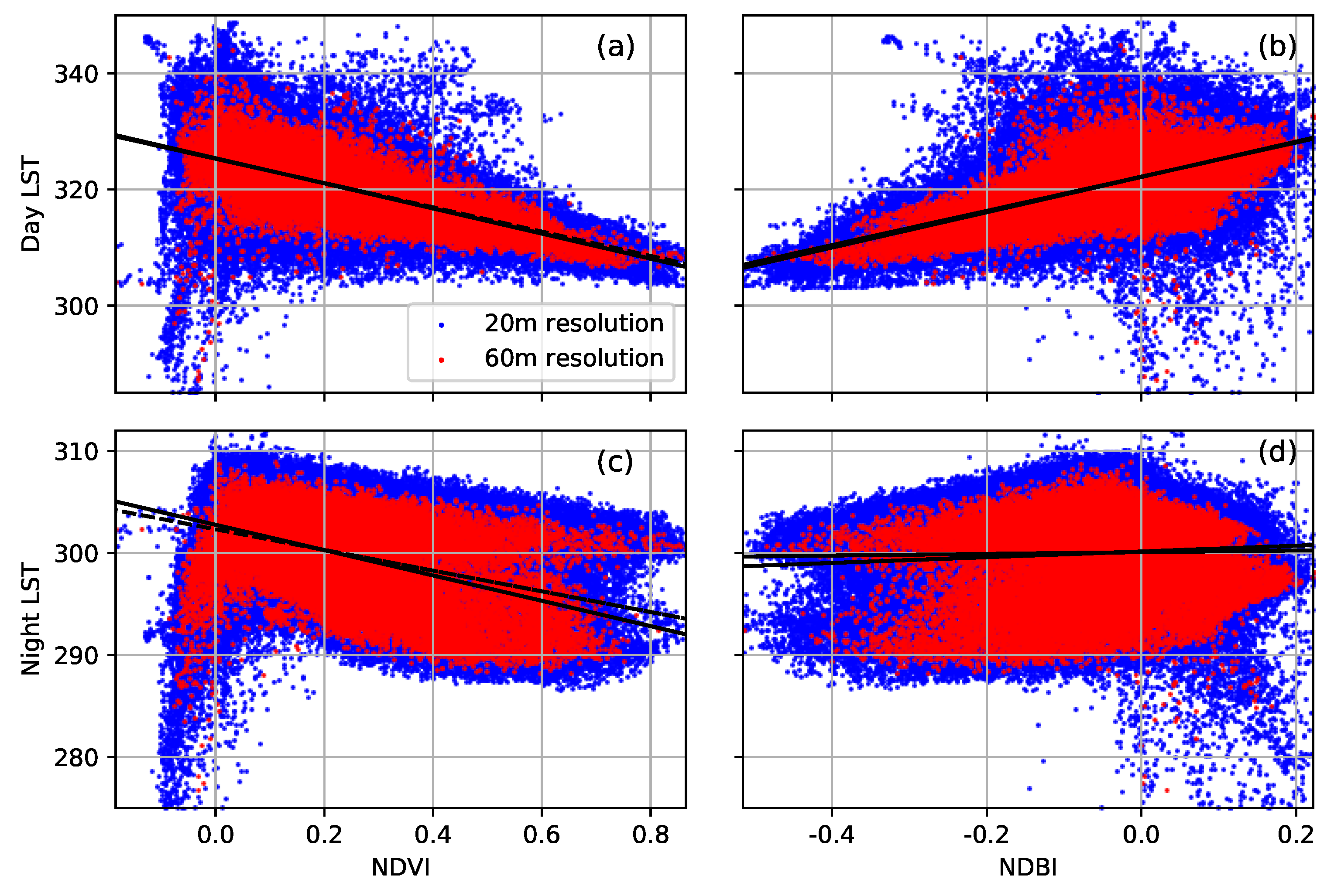
4.1. Night-LST vs. Day-Index Regressions

4.1.1. Global Linear Behavior: DisTrad and ATPRK

Figure 3a,b show the behavior of day-LST on NDVI and NDBI respectively at 20 m resolution in blue and 60 m resolution in red. During day, the range of LSTs varies from 300 to 340 K. The behavior of day-LST on NDVI or NDBI can be supposed linear (black lines) with a dense region of points when $NDVI>0.5$ ($NDBI<-0.3$) and temperatures between 300 and 320 K. These pixels correspond to vegetation. When NDVI decreases (NDBI increases) the possible LSTs for a given index value become sparser. These pixels correspond to impervious surfaces, whose temperature can behave in a very different way depending on their composition and sun exposure.

Figure 3c,d show the behavior of night-LST on NDVI and NDBI respectively. During the night, the range of LSTs varies from 285 to 310 K. The range of LSTs has considerably varied from day to night, with a decrease in temperature of about 30 K. The denser region found during day when $NDVI>0.5$ ($NDBI<-0.3$) disappears in night figures, and for any index value the range of possible LST goes from 290 to 310. In addition, the linear behavior of LST on NDVI (NDBI) becomes unclear. During the night, the temperatures globally decrease. In addition, a higher sparsity of LSTs in function of NDVI (NDBI) is found. This higher sparsity is explained on one hand by the high thermal inertia of vegetation, which produces the sparsity of LSTs in the right side of Figure 3c,d, and on the other hand, on the low thermal inertia of impervious surfaces, which can decrease 30 K from day to night and whose sparsity also increases.

For both day and night, pixels with LST below 300 and 285 K respectively correspond to metallic surfaces whose LST is hard to estimate and the obtained values should not be considered.

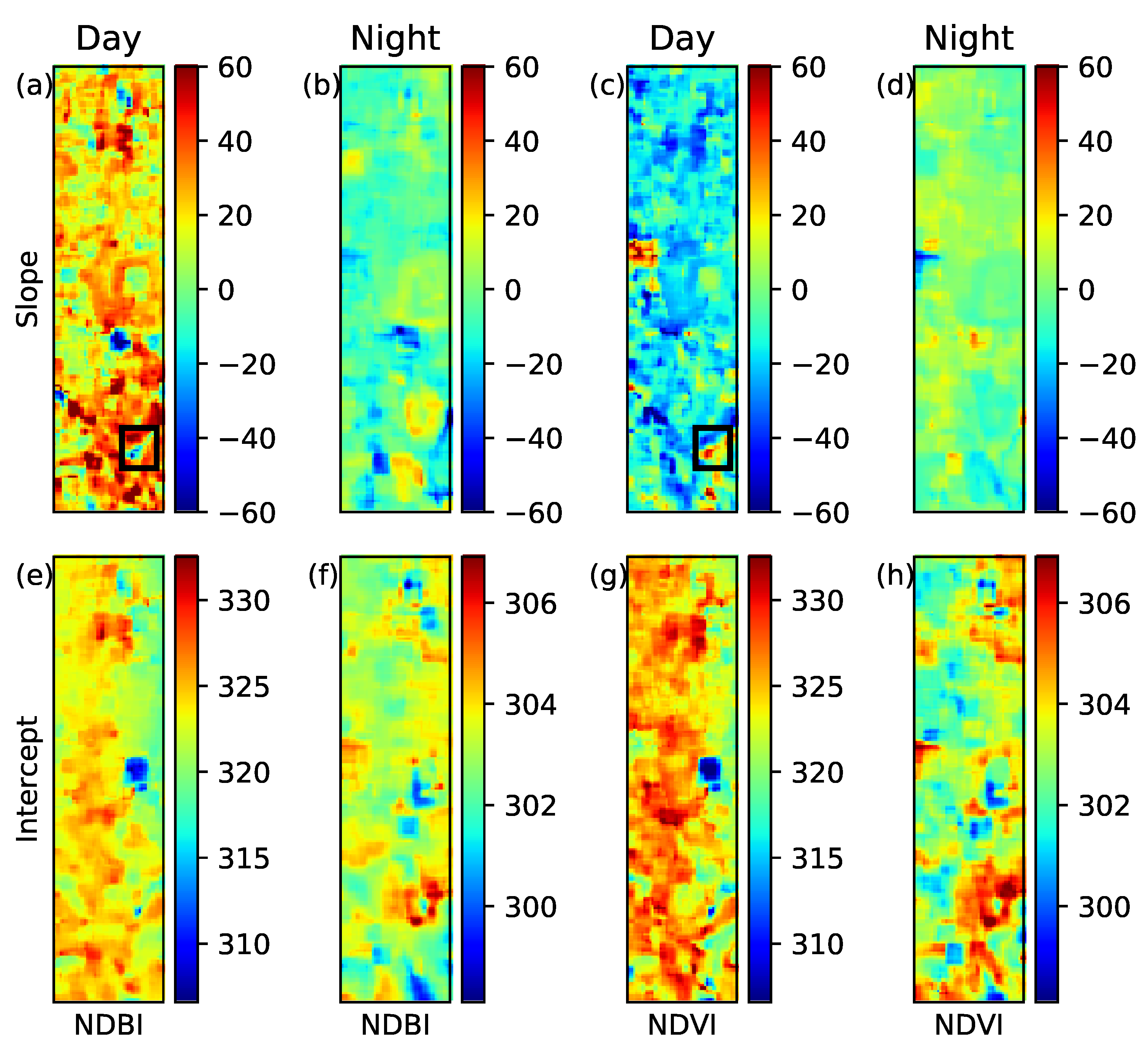
4.1.2. Local Linear Behavior: AATPRK

The performance of AATPRK has been studied in function of the size of the window where the LST-index regression is done, see Equation (4). Window sizes of $N=9$ ($3\times 3$), $N=25$ ($5\times 5$), $N=49$ ($7\times 7$) and $N=81$ ($9\times 9$) were evaluated, finding the $N=49$ size slightly more performant. Throughout this article, only results of AATPRK with $N=49$ are shown.

Figure 4a–d presents the local slopes obtained with AATPRK using NDBI ((a) and (b)) and NDVI ((c) and (d)) as reflective indices and for day and night images respectively. Very interestingly, Figure 4c,d show that while day-LST vs. NDVI slopes are mainly negatives, those of night-LST are mainly positives, indicating an inversion of the sign of the slope in the regression. This effect of slope inversion is also found in local LST-NDBI regressions (Figure 4a,b). Negative daytime slopes with NDVI, respectively positive with NDBI, are related to regression windows where pixels with high NDVI (low NDBI) present low temperatures. This behavior is expected when high NDVI (low NDBI) values correspond to vegetated (at least partially) pixels. However, in urban environments, materials with high NDVI (low NDBI) and high temperature, or viceversa, are present. The existence of these materials leads to urban pixels influencing the LST-index slope for day LSTs, see for example the Atocha railways (with metallic buildings) in the area framed by the black squares of Figure 4a,c. On the other hand, the inversion of the slope between day and night LST regressions is related to the low thermal inertia of impervious materials, which (depending on their placement: urban canyon geometry, shadows) reach high temperatures during day, but low temperatures during the night. This inversion of the slope’s sign does not appear in non-local LST-index regression (Figure 3a–d). In addition, local day-LST vs. NDBI globally presents higher (in modulus) slopes than its night version (Figure 4a,b). This effect is also found in the non-local linear LST-NDBI regression (Figure 3b,d).

Figure 4e–h shows the intercept of LST in function of NDBI ((e) and (f)) and NDVI ((g) and (h)) during day and night respectively. The hotter regions obtained with the day regression correspond to the cooler regions for the night one. Equivalently, the cooler regions for the day regression correspond to the hotter regions during the night. This result is explained by the low thermal inertia of the impervious materials that are found in the red regions of Figure 4e,g, and the high thermal inertia of the green ones. These red regions consist of Madrid old town and close neighborhoods composed by small and narrow streets with few vegetation, while the green regions correspond to wider avenues containing trees.

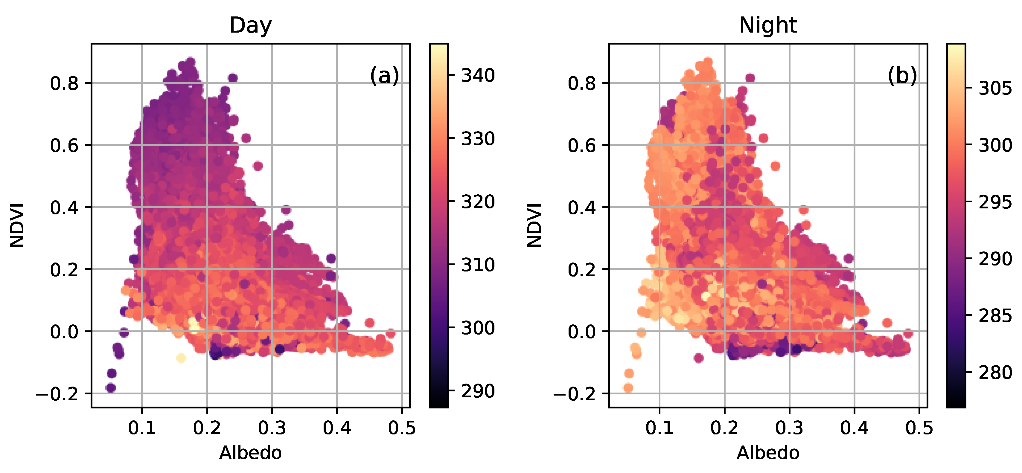
4.1.3. Polynomial Behavior: HUTS

Figure 5a,b shows respectively the day and night LST vs. {NDVI, Albedo}. For both figures, NDVI and Albedo are measured during day, and therefore the samples positions in the day and night plots are unchanged. However, this is not the case for the LSTs (color map). Night-LSTs (∈ (280, 305 K)) are cooler than day-LSTs (∈ (290, 340 K)), and many day samples with cool temperatures appear as night samples with warm temperatures. This effect is again a footprint of the differences in thermal inertia.

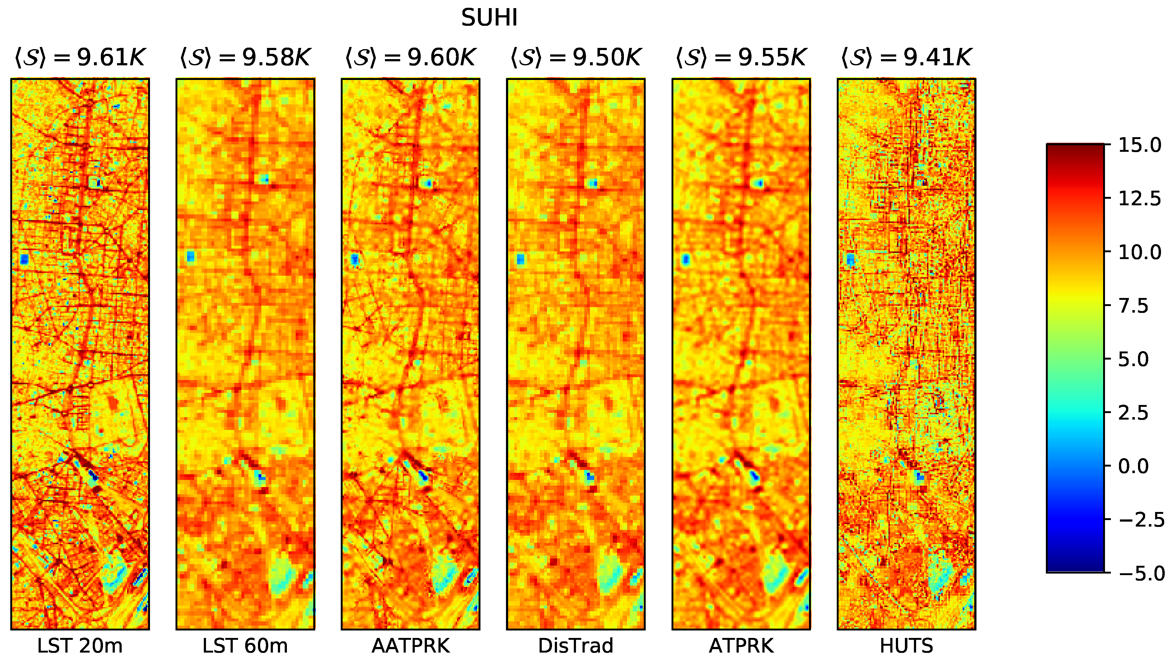
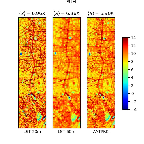
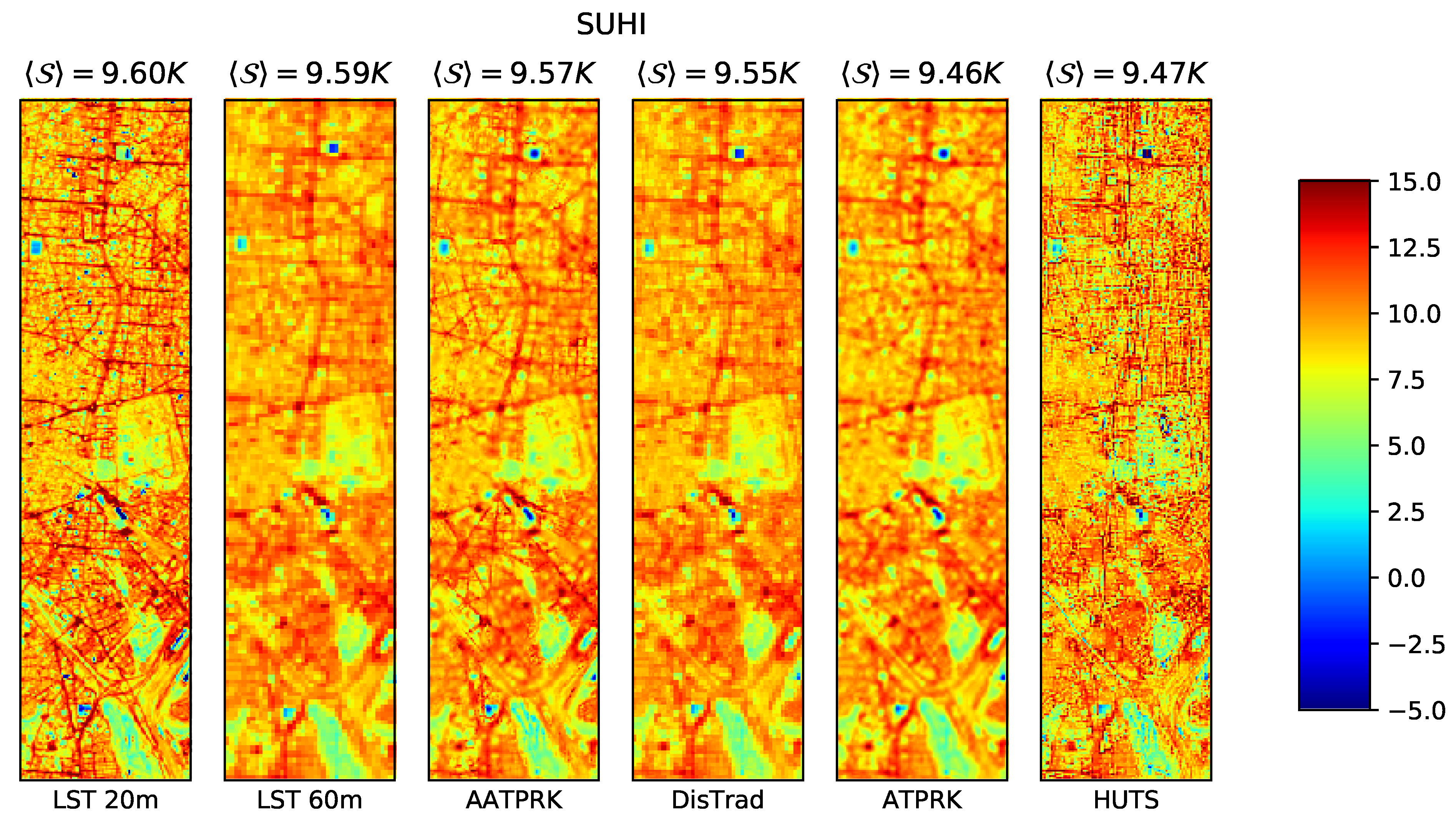
4.2. SUHI Estimation from Unmixed Night-LST

In this section, microscale and classical SUHI in Madrid city center are obtained from unmixed LSTs following the methodology explained in Section 3.3. For DisTrad, ATPRK, and AATPRK the used reflective index is NDBI, while for HUTS the used indices are NDVI and Albedo such as in [19].

Figure 6 shows the microscale SUHI values and the classical SUHI value obtained by averaging, both estimated from different LST images. From left to right: reference LST at 20 m resolution, LST at 60 m resolution, and LSTs at 20 m obtained from 60 m with AATPRK, DisTrad, ATPRK, and HUTS. On one hand, the classical SUHI values are very close, $〈\mathcal{S}〉\in [9.46,9.60]$ K, being in any case higher than the classical SUHI estimated from the AHS image at 4 m resolution, $〈{\mathcal{S}}_{4m}〉=9.2$ K. On the other hand, the microscale SUHIs present differences. DisTrad and ATPRK present microscale SUHI estimations that are visually closer to the coarse 60 m resolution estimation than to the reference one at 20 m, appearing that no unmixing was performed. This effect can be explained by the weak slope of the night-LST vs. NDBI regression (Figure 3d). For a given coarse pixel, the LSTs of finer pixels within it are mainly defined by the intercept of the regression, which is independent of the index value of the fine pixels.

HUTS misestimates the street pavements temperatures, finding colder temperatures in the streets than in the roofs. This temperature reversal effect is explained by two reasons: first, the shadows, largely covering the streets during day (and not at all the roofs), influence the indices estimation, second, the low thermal inertia of these materials leads to important changes between day and night temperatures of the sun exposed pixels, which can conduct to the loss of the night-LST versus day-index relationship. This effect is not only found with HUTS but with DisTrad and ATPRK when NDVI is used in the regression. Furthermore, other vegetation indices such as Fractional Cover (FC) [18], or Enhanced Vegetation Index (EVI) [36], have been tested giving similar results.

On the other hand, AATPRK, performing local regressions, presents microscale SUHI estimations that are closer to the reference fine resolution one. An important number of streets, which were lost in the 60 m resolution image and in the DisTrad and ATPRK unmixed ones, are recovered, as well as the dynamic of the LST, with hotter LSTs in the streets than in the buildings. The good results obtained with AATPRK using NDBI as regression index are also obtained if NDBI is replaced by NDVI. Therefore, when local regressions are performed (AATPRK), vegetation indices do not lead to street pavement LSTs misestimation. While for global regressions (DisTrad, ATPRK, and HUTS) LST-NDVI behavior is the same for day and night images, i.e., both the day and night slopes are negative (Figure 3a,c), this is no longer the case for local regressions (AATPRK) in the urban environment, see Figure 4c,d. For AATPRK, the behavior of LST-NDVI is inversed, i.e., negative slope during day and positive slope during the night, and leads to a good LST unmixing. The better performances of AATPRK can thus be explained because while local regressions take into account the structure of the area around the pixel (shadows, urban canyon geometry, vegetation, impervious materials), global regressions do not take into account this structure, which can strongly vary from one point to another in the image. Thus, local LST-index regression is most performant because the urban structure and composition, which influence the LST-index relationship, are closer for the pixels used in the regression.

These results are supported by Figure 7, which shows the microscale SUHI profile measured from west to east between Glorieta de Embajadores and Atocha train station (magenta line in Figure 1) for the different unmixed LSTs (markers: points for unmixed LST and crosses for unmixed LST without residual correction) together with the reference microscale SUHI at 20 m resolution (blue line). AATPRK presents the most similar profile to the 20 m reference one, followed by ATPRK. However, a spatial smoothing of the microscale SUHI profiles obtained with DisTrad and ATPRK is found. This smoothing, which is not found with AATPRK, can be due to the weakness of the unmixing performed with these methods (Figure 6): all fine pixels within a coarse one present very similar behavior and then variations within a coarse pixel influence all the fine pixels inside. Microscale SUHI profile obtained with HUTS presents a behavior far from the reference profile, with lower and higher aberrant temperature values. Figure 7 also shows the importance of residual correction for the non-local methods: DisTrad, ATPRK, and HUTS. While for AATPRK the residual correction slightly improves the LST unmixing, this correction appears as essential for the other three methods.

Table 2. Root mean square error (RMSE), mean bias error (MBE), cross correlation (R), and Structural Similarity Index (SSIM) for 20 m Land Surface Temperature (LST) images unmixed from 60 m resolutions with different unmixing techniques and for 60 m LST resolution. A 20 m LST image is used as reference. “City center” indicates that only the values within the red rectangle of Figure 1 are taken into account, while “Whole image” considers all the pixels of Figure 1.

28/06/2008
City Center
Unmixing Resolutions	Method	RMSE (K)	MBE (K)	R	SSIM
60 m → 20 m	DisTrad	1.63	0.02	0.73	0.32
	ATPRK	1.49	0.04	0.78	0.40
	AATPRK	1.43	−0.00	0.80	0.48
	HUTS	2.73	0.03	0.40	0.09
60 m		1.58	0.02	0.75	0.36
Whole Image
Unmixing Resolutions	Method	RMSE (K)	MBE (K)	R	SSIM
60 m → 20 m	DisTrad	1.67	0.02	0.92	0.41
	ATPRK	1.53	0.02	0.93	0.50
	AATPRK	1.49	−0.00	0.94	0.53
	HUTS	2.58	−0.05	0.78	0.33
60 m		2.65	−0.02	0.88	0.42

shows the quantitative results (RMSE, MBE, R, and SSIM) characterizing the similarity between the 20 m reference LST and the unmixed night LSTs. The similarity between the 20 m reference LST and the coarse scale (60 m) LST is also shown. Two cases are studied: on one hand a pure urban case, by analyzing only the city center of Madrid (red rectangle of Figure 1), on the other hand the whole scene (Figure 1) is studied. For both cases, AATPRK appears as the most performant technique followed very closely by ATPRK. DisTrad appears as better than the coarse image at 60 m but worse than ATPRK and AATPRK, while HUTS appears even worse than the initial coarse image due to the misestimation explained above. One local quantity (SSIM) and three global quantities (RMSE, MBE, and R) have been used to discriminate between unmixing techniques. However, although the quantitative discrimination between the couple AATPRK/ATPRK and the other two techniques have been done, the used quantities are not able to discriminate between AATPRK and ATPRK, even if visually the differences are shown.

The unmixing methods used in this article incorporate several hypotheses (LST-index relationship, scale-invariance of the regression parameters, and residual estimation hypotheses), and their final performances will depend on the better or worse validity of all of them [21]. For night-LST unmixing, both the locality of the method and the used reflective index appear as major factors influencing the unmixing performance. Another important aspect is the computation time of each unmixing method, which should be taken into account when large images are processed. In this respect, DisTrad appears as the fastest technique with a computation time of 18 s when unmixing the night-LST image of the 28 June. HUTS needs 77 s to unmix the same night-LST image, while ATPRK with 556 s and AATPRK with 981 s show the main disadvantage of area-to-point residual estimation. All these computation times have been estimated by averaging over 15 realizations.

Finally, this characterization of the microscale SUHIs of Madrid city center, obtained through thermal unmixing, allows at least two observations. First, urban canyon geometry implies warmer LSTs for street pavement than for roofs, independently of the neighborhood and when the street is wide enough. Second, vegetation does not appear as a major cooling driver during the night, but mostly like a regulatory body. Indeed, vegetation, having a higher thermal inertia than most of the impervious materials, preserves the heat acquired during the day better. Thus, it is possible to find that the temperature of vegetated regions, being cooler than the temperature of non-vegetated areas during daytime, becomes warmer or at least equal during the night. This effect can be seen in some parts of the Retiro Park (yellow rectangle of Figure 1).

5. Conclusions

In this article, four empirical thermal unmixing methods (DisTrad, ATPRK, AATPRK, and HUTS) based on given relationships between LST and reflective indices, are adapted to unmix night LSTs. It is shown that the application of these thermal unmixing methods on night time images is not straightforward. This is mainly due to the different ranges of day and night temperatures and the different thermal inertia of impervious and vegetation materials which influence the validity of the LST-indices relationships when the LST is estimated during the night and the indices during day. Between the four studied methods only AATPRK noticeably improves the night temperature characterization of the city. This is due to the local application of the method which, contrary to the others, works on LST-index relationships within a sliding window. The locality of the night LST-index relationship seems decisive for the correctness of the unmixing.

Another important factor is the choice of the day reflective index used in the unmixing. Even if for day-LST unmixing vegetation and built-up indices appear to have similar performances (with NDBI performing only slightly better) [21], this is not the case for night-LST unmixing. NDBI, incorporating information from the SWIR band, describes the structure of the city better and its relationship with LST is better preserved from day to night. LST misestimation effects are found with DisTrad, ATPRK, and HUTS when using vegetation indices, i.e., street pixels are obtained as cooler than roof pixels. These reversal effects do not appear with AATPRK when using vegetation indices. However, this may not be always the case, and the appearance of this effect with AATPRK would depend on the size of the local window where the night-LST day-index regression is performed, and also on the local roughness of the city. In this work, the most performant window size was found to be $7\times 7$ pixels, while Ribeiro-Pereira et al., 2018 [23] found $5\times 5$ for LST unmixing over the urban area of Campo Grande in Brazil. So, the size of the window used in AATPRK should be adapted in function of the studied city, since the most performant size will depend on the urban structure and composition. The evaluation of the impact of the window size on AATPRK performances over different cities is needed to obtain general conclusions.

A good registration of day-night images is also central for night LST unmixing, since small deviations in the day-index night-LST repositioning can induce larger errors in the final outcomes. The study of these misregistrations will be evaluated in future works.

The principal interest of performing night-LST unmixing is the study of urban climatology and more precisely the characterization of microscale SUHIs. Thus, night LST unmixing with AATPRK using daytime reflective information allows a better study of these microscale SUHIs. It allows one to discriminate narrower streets and buildings, and thus to obtain information from urban objects such as small parks or sport centers which are lost without unmixing. This can provide a better understanding of the drivers leading to temperature increases.

The performances of these unmixing methods applied on night LST images from less resoluted satellites (ASTER, MODIS) should be analyzed in future works, as well as their performances on cities with different structural and climatological characteristics.

References

1. Rizwan, A.; Dennis, L.; Chunho, L. A review on the generation, determination and mitigation of urban heat island. J. Environ. Sci. 2008, 20, 120–128. [Google Scholar] [CrossRef]
2. Hart, M.; Sailor, D. Quantifying the influence of land-use and surface characteristics on spatial variability in the urban heat island. Theor. Appl. Climatol. 2009, 95, 397–406. [Google Scholar] [CrossRef]
3. Huang, H.; Ooka, R.; Kato, S. Urban thermal environment measurements and numerical simulation for an actual complex urban area covering a large district heaheat and cooling system in summer. Atmos. Environ. 2005, 39, 6362–6375. [Google Scholar] [CrossRef]
4. Sarrat, C.; Lemonsu, A.; Masson, V.; Guedalia, D. Impact of urban heat island on regional atmospheric pollution. Atmos. Environ. 2006, 40, 1743–1758. [Google Scholar] [CrossRef]
5. Kolokotroni, M.; Zhang, Y.; Watkins, R. The London heat island and building cooling design. Sol. Energy 2007, 81, 102–110. [Google Scholar] [CrossRef]
6. Priyadarsini, R. Urban heat island and its impact on building energy consumption. Adv. Build. Energy Res. 2009, 3, 261–270. [Google Scholar] [CrossRef]
7. Stone, B.; Norman, J. Land use planning and surface heat island formation: A parcel-based radiation flux approach. Atmos. Environ. 2006, 40, 3561–3573. [Google Scholar] [CrossRef]
8. Kim, J.; Guldmann, J. Land-use planning and the urban heat island. Environ. Plan. B Urban Anal. City Sci. 2014, 41, 1077–1099. [Google Scholar] [CrossRef]
9. Anniballe, R.; Bonafoni, S.; Pichierri, M. Spatial and temporal trends of the surface and air heat island over Milan using MODIS data. Remote Sens. Environ. 2014, 150, 163–171. [Google Scholar] [CrossRef]
10. Jin, M.; Dickinson, R. Land surface skin temperature climatology: Benefitting from the strengths of satellite observations. Environ. Res. Lett. 2010, 5, 044004. [Google Scholar] [CrossRef]
11. Tiangco, M.; Lagmay, A.; Argete, J. ASTER-based study of the night-time urban heat island effect in Metro Manila. Int. J. Remote Sens. 2008, 29, 2799–2818. [Google Scholar] [CrossRef]
12. Sobrino, J.; Oltra-Carrió, R.; Sòria-Barres, G.; Jiménez-Muñoz, J.C.; Franch, B.; Hidalgo, V.; Mattar, C.; Julien, Y.; Cuenca, J.; Romaguera, M.; et al. Evaluation of the surface urban heat island effect in the city of Madrid by thermal remote sensing. Int. J. Remote Sens. 2013, 34, 3177. [Google Scholar] [CrossRef]
13. Lagouarde, J.; Bhattacharya, B.; Crebassol, P.; Gamet, P.; Babu, S.; Boulet, G.; Briottet, X.; Buddhiraju, K.M.; Cherchali, S.; Dadou, I.; et al. The Indian–French Trishna mission: Earth observation in the thermal infrared with high spatio-temporal resolution. In Proceedings of the IEEE International Geoscience and Remote Sensing Symposium IGARSS, Valencia, Spain, 22–27 July 2018. [Google Scholar]
14. Koetz, B.; Bastiaanssen, W.; Berger, M.; Defourny, P.; Bello, U.D.; Drusch, M.; Drinkwater, M.; Duca, R.; Fernandez, V.; Ghent, D.; et al. High spatio-temporal resolution land surface temperature mission—A Copernicus candidate mission in support of agricultural monitoring. In Proceedings of the IEEE International Geoscience and Remote Sensing Symposium IGARSS, Valencia, Spain, 22–27 July 2018. [Google Scholar]
15. Lee, C.; Cable, M.; Hook, S.; Green, R.; Ustin, S.; Mandl, D.; Middleton, E. An introduction to the NASA Hyperspectral Infrared Imager (HyspIRI) mission and preparatory activities. Remote Sens. Environ. 2015, 167, 6–19. [Google Scholar] [CrossRef]
16. Welch, R. Spatial resolution requirements for urban studies. Int. J. Remote Sens. 1982, 3, 139–146. [Google Scholar] [CrossRef]
17. Zhan, W.; Chen, Y.; Zhou, J.; Wang, J.; Liu, W.; Voogt, J.; Zhu, X.; Quan, J.; Li, J. Disaggregation of remotely sensed land surface temperature: Literature survey, taxonomy, issues and caveats. Remote Sens. Environ. 2013, 131, 119–139. [Google Scholar] [CrossRef]
18. Agam, N.; Kustas, W.P.; Anderson, M.; Li, F.; Neale, C. A vegetation index based technique for spatial sharpening of thermal imagery. Remote Sens. Environ. 2007, 107, 545–558. [Google Scholar] [CrossRef]
19. Dominguez, A.; Kleissl, J.; Luvall, J.C.; Rickman, D.L. High-Resolution Urban Thermal Sharpener (HUTS). Remote Sens. Environ. 2011, 115, 1772–1780. [Google Scholar] [CrossRef]
20. Wang, Q.; Shi, W.; Atkinson, P.M. Area-to-point regression kriging for pan-sharpening. ISPRS J. Photogramm. Remote Sens. 2016, 114, 151–165. [Google Scholar] [CrossRef]
21. Granero-Belinchon, C.; Michel, A.; Lagouarde, J.P.; Sobrino, J.; Briottet, X. Multi-resolution study of thermal unmixing techniques over Madrid urban area: Case study of TRISHNA mission. Remote Sens. 2019, 11, 1251. [Google Scholar] [CrossRef]
22. Wicki, A.; Parlow, E. Multiple regression analysis for unmixing of surface temperature data in an urban environment. Remote Sens. 2017, 9, 684. [Google Scholar] [CrossRef]
23. Pereira, O.; Melfi, A.; Montes, C.; Lucas, Y. Downscaling of ASTER thermal images based on geographically weighted regression kriging. Remote Sens. 2018, 10, 633. [Google Scholar] [CrossRef]
24. Essa, W.; Verbeiren, B.; van der Kwast, J.; van de Voorde, T.; Batelaan, O. Evaluation of the DisTrad thermal sharpening methodology for urban areas. Int. J. Appl. Earth Obs. Geoinf. 2012, 19, 163–172. [Google Scholar] [CrossRef]
25. Wang, Q.; Shi, W.; Atkinson, P.M.; Zhao, Y. Dowsncaling MODIS images with area-to-point regression kriging. Remote Sens. Environ. 2015, 166, 191–204. [Google Scholar] [CrossRef]
26. Sobrino, J.; Bianchi, R.; Paganini, M.; Sòria, G.; Jiménez-Muñoz, J.; Oltra-Carrió, R.; Mattar, C.; Romaguera, M.; Franch, B.; Hidalgo, V.; et al. DESIREX 2008: Dual-use European Security IR Experiment 2008; Technical Report; European Space Agency: Paris, France, 2009. [Google Scholar]
27. Sobrino, J.; Bianchi, R.; Paganini, M.; Sòria, G.; Oltra-Carrió, R.; Romaguera, M.; Jiménez-Muñoz, J.; Cuenca, J.; Hidalgo, V.; Franch, B.; et al. Urban Heat Island and Urban Thermography project DESIREX 2008. In Proceedings of the 33rd International Symposium on Remote Sensing of Environment, ISRSE, Stresa, Italy, 4–8 May 2009. [Google Scholar]
28. Oltra-Carrió, R. Thermal Remote Sensing of Urban Areas. The Case Study of the Urban Heat Island of Madrid. Ph.D. Thesis, Universitat de Valencia, Valencia, Spain, 2013. [Google Scholar]
29. Miesch, C.; Poutier, L.; Achard, V.; Briottet, X.; Lenot, X.; Boucher, Y. Direct and Inverse Radiative Transfer solutions for visible and near-infrared hyperspectral imagery. IEEE Trans. Geosci. Remote Sens. 2005, 43, 1552–1562. [Google Scholar] [CrossRef]
30. Zhang, X.; Zhong, T.; Wang, K.; Cheng, Z. Scaling of impervious surface area and vegetation as indicators to urban land surface temperature using satellite data. Int. J. Remote Sens. 2009, 30, 841–859. [Google Scholar] [CrossRef]
31. Gillespie, A.; Rokugawa, S.; Matsunaga, T.; Cothern, J.S.; Hook, S.; Kahle, A.B. A temperature and emissivity separation algortihm for advanced spaceborn thermal emission and reflection radiometer (ASTER) images. IEEE Trans. Geosci. Remote Sens. 1998, 36, 1113–1126. [Google Scholar] [CrossRef]
32. Kustas, W.P.; Norman, K.M.; Anderson, M.C.; French, A.N. Estimating subpixel surface temperatures and energy fluxes from the vegetation index—Radiometric temperature relationship. Remote Sens. Environ. 2003, 85, 429–440. [Google Scholar] [CrossRef]
33. Essa, W.; Verbeiren, B.; van der Kwast, J.; Batelaan, O. Improved DisTrad for downscaling thermal MODIS imagery over urban areas. Remote Sens. 2017, 9, 1243. [Google Scholar] [CrossRef]
34. Ben-Dor, E.; Saaroni, H. Airborne video thermal radiometry as a tool for monitoring microscale structures of the urban heat island. Int. J. Remote Sens. 1997, 18, 3039–3053. [Google Scholar] [CrossRef]
35. Wang, Z.; Bovik, A.C. Mean Squared Error: Love it or leave it? IEEE Signal Process. Mag. 2009, 26, 98–117. [Google Scholar] [CrossRef]
36. Liu, H.; Huete, A. A feedback based modification of the NDVI to minimize canopy background and atmospheric noise. IEEE Trans. Geosci. Remote Sens. 1995, 33, 457–465. [Google Scholar]
Figure 1. Madrid (Spain) Airborne Hyperspectral Scanner RGB image from Getafe (south) to Universidad Autónoma (north) at 4 m resolution. The red rectangle corresponds to the city center shown in the results section for visual analysis. The green rectangle corresponds to the region used to estimate countryside Land Surface Temperature (LST). The magenta line corresponds to the region shown in the results for profile inspection. The yellow rectangle frames the Retiro Park, which is one of the largest parks in the city of Madrid.
Remotesensing 11 01449 g001
Figure 2. Diagram of the research methodology. Reflective day image processing in green. Thermal InfraRed (TIR) night image processing in red. Unmixing steps in orange. Surface urban heat islands (SUHIs) estimations in blue.
Remotesensing 11 01449 g002
Figure 3. Linear behavior of LST versus index. (a,b) show day-LST versus Normalized Difference Vegetation index (NDVI) and Normalized Difference Built-Up Index (NDBI) respectively and (c,d) show night-LST versus NDVI and NDBI respectively. Red dots for 60 m resolution pixels and blue dots for 20 m resolution pixels. Black lines correspond to linear regressions, dashed for 20 m and continuous for 60 m. Both, day and night data correspond to the pixels of the whole image, see Figure 1.
Remotesensing 11 01449 g003
Figure 4. Slope and intercept values of Adaptive Area-To-Point Regression Kriging (AATPRK) regressions at 60 m resolution for Madrid city center (red rectangle of Figure 1). (a,b) show respectively the slope of day and night LST versus NDBI; (c,d) show the slope of day and night LST versus NDVI; (e,f) show the intercept of day and night LST versus NDBI; (g,h) show the intercept of day and night LST versus NDVI.
Remotesensing 11 01449 g004
Figure 5. Polynomial behavior of LST versus {NDVI, Albedo} at 60 m resolution. (a) day-LST vs. {NDVI, Albedo} (b) night-LST vs. {NDVI, Albedo}. Both day and night data correspond to the pixels of the whole image, see Figure 1.
Remotesensing 11 01449 g005
Figure 6. Madrid city center microscale and classical SUHIs studied at 20 m, 60 m, and from unmixing: AATPRK, Disaggregation of radiometric surface Temperature (DisTrad), Area-To-Point Regression Kriging (ATPRK), and High-resolution Urban Thermal Sharpener (HUTS) at 20 m from 60 m.
Remotesensing 11 01449 g006
Figure 7. Madrid city center west-east microscale SUHI profile for the four tested unmixing techniques (color points) together with the reference SUHI at 20 m (blue line). The profile is measured between Glorieta de Embajadores and Atocha train station (magenta line in Figure 1). The color crosses correspond to the unmixing results without residual correction.
Remotesensing 11 01449 g007