Article

Monitoring the Variation of Vegetation Water Content with Machine Learning Methods: Point–Surface Fusion of MODIS Products and GNSS-IR Observations

1
School of Geodesy and Geomatics, Wuhan University, Wuhan 430079, China
2
Key Laboratory of Geospace Environment and Geodesy, Ministry of Education, Wuhan University, Wuhan 430079, China
3
Faculty of Information Engineering, China University of Geosciences, Wuhan 430074, China
4
School of Resource and Environmental Sciences, Wuhan University, Wuhan 430079, China
5
The Collaborative Innovation Center for Geospatial Technology, Wuhan 430079, China
6
The Key Laboratory of Geographic Information System, Ministry of Education, Wuhan University, Wuhan 430079, China
7
The State Key Laboratory of Information Engineering in Surveying, Mapping and Remote Sensing, Wuhan University, Wuhan 430079, China
*
Author to whom correspondence should be addressed.
Remote Sens. 2019, 11(12), 1440; https://doi.org/10.3390/rs11121440
Submission received: 5 May 2019 / Revised: 10 June 2019 / Accepted: 13 June 2019 / Published: 18 June 2019

Abstract

:
Vegetation water content (VWC) is recognized as an important parameter in vegetation growth studies, natural disasters such as forest fires, and drought prediction. Recently, the Global Navigation Satellite System Interferometric Reflectometry (GNSS-IR) has emerged as an important technique for monitoring vegetation information. The normalized microwave reflection index (NMRI) was developed to reflect the change of VWC based on this fact. However, NMRI uses local site-based data, and the sparse distribution hinders the application of NMRI. In this study, we obtained a 500 m spatially continuous NMRI product by integrating GNSS-IR site data with other VWC-related products using the point–surface fusion technique. The auxiliary data in the fusion process include the normalized difference vegetation index (NDVI), gross primary productivity (GPP), and precipitation. Meanwhile, the fusion performance of three machine learning methods, i.e., the back-propagation neural network (BPNN), generalized regression neural network (GRNN), and random forest (RF) are compared and analyzed. The machine learning methods achieve satisfactory results, with cross-validation R values of 0.71–0.83 and RMSEs of 0.025–0.037. The results show a clear improvement over the traditional multiple linear regression method, which achieves R (RMSE) values of only about 0.4 (0.045). It indicates that the machine learning methods can better learn the complex nonlinear relationship between NMRI and the input VWC-related index. Among the machine learning methods, the RF model obtained the best results. Long time-series NMRI images with a 500 m spatial resolution in the western part of the continental U.S. were then obtained. The results show that the spatial distribution of the NMRI product is consistent with a drought situation from 2012 to 2014 in the U.S., which verifies the feasibility of analyzing and predicting drought times and distribution ranges by using the 500 m fusion product.

Graphical Abstract

1. Introduction

In recent years, with the development of imaging spectrometry, using remote sensing data to detect the chemical characteristics of vegetation has become an important topic in the study of global change. Vegetation water content (VWC) has been recognized as a key variable for assessing crop physiological status, due to its close association with plant transpiration, photosynthesis, vegetation stress, and biomass productivity [1]. The water deficit directly affects the physiological and biochemical processes and morphological structures of plants, thus affecting growth. Knowledge of vegetation moisture can guide accurate irrigation, forecast yield, evaluate natural droughts, and predict forest fires and other natural disasters [2,3]. Therefore, the estimation of high-precision and long time-series VWC products, especially during key phenological stages, is important for vegetation research. The conventional field-based methods for VWC measurement are destructive and labor-intensive, especially in large areas with great within-field variabilities in soil infiltration characteristics or microtopography [4]. As an alternative, remote sensing techniques, with which it is easier to acquire long time-series VWC spatial information over a wide range nondestructively, can overcome the above shortcomings [5].
There is a long history of using remote sensing data to estimate vegetation water information. Commonly used remote sensing technologies include optical and microwave remote sensing. The former refers to the remote sensing technology that detects the target surface objects by using the reflection characteristics of the visible light band. The latter refers to the remote sensing technology of microwave electromagnetic wave with a wavelength of 1~1000 mm and can be divided into active remote sensing and passive remote sensing according to its working principles. For optical remote sensing, some empirical methods exploit the obvious correlation between biophysical parameters, such as the Normalized Difference Vegetation Index (NDVI) [6], land surface temperature (LST) [7], and other variables, to assess VWC. Moreover, a reduction in VWC will cause variations in spectral reflectance. Red, the near-infrared (NIR), and the short-wave infrared (SWIR) bands are sensitive to vegetation water stress and are used to compose various water indices to indicate VWC [8]. Common indices include the normalized difference water index (NDWI) [9], the normalized difference infrared index (NDII) [10], the simple ratio water index (SRWI) [11], and the global vegetation water moisture index (GVMI) [12]. Meanwhile, microwave remote sensing also has been used to estimate VWC, since the dielectric constant of water and dry vegetation differs significantly, and thus the amount of water stored in vegetation directly affects how microwave radiation interacts with vegetation canopies. For active microwave remote sensing, studies have shown that the scattering coefficients and the polarization of signals are sensitive to VWC [13]. Kim et al. [14] and Srivastava et al. [15] suggested that retrieving VWC using the L-band radar vegetation index (RVI) and HV radar backscattering was feasible. For passive microwave remote sensing, researchers have also illustrated the feasibility of detecting VWC based on brightness temperature, owing to its effect on the emissivity of the canopy [16,17].
Although the spatial resolution of VWC obtained by optical remote sensing inversion is usually high, the optical images are vulnerable to cloud and fog, resulting in missing information. In comparison, owing to the long wavelength of microwave signals, they usually have strong penetrative abilities and are not affected by cloud cover. However, microwave signals can not only penetrate clouds, but also the thickest vegetation canopies, and, therefore, the measured vegetation information from microwave signals is affected by the roughness of the ground, soil moisture, and other factors [18]. Furthermore, compared with optical-based data, microwave data usually have a coarse spatial resolution, which limits their potential in some fine-scale applications. In recent years, there have been some studies combining these two kinds of data to retrieve VWC with a higher resolution [19,20]; however, the huge spatial resolution difference between optical and microwave remote sensing products makes the accuracy and spatial resolution of the fusion results poor in practical applications. Therefore, other superior methods to retrieve VWC are needed.
Global Navigation Satellite System Interferometric Reflectometry (GNSS-IR) provides us with a new mode to monitor the vegetation information in a long time series. It acts as a relatively new L-band remote sensing technique with relevance for measuring vegetation state using reflected GNSS signals by recording the interference between a direct GNSS signal and a reflected GNSS signal [21]. Daily VWC information can be acquired in a network named EarthScope Plate Boundary Observatory (PBO) H2O based on GNSS-IR technique [21]. Martin [22] first proposed to use reflected GPS signals to measure sea level from space in 1993. It was subsequently expanded to a variety of ground, aircraft, and space-based platforms for studies of soil moisture [23], ocean winds [24], sea ice [25], ocean tides [26,27], snow [28], and vegetation. For vegetation, many researchers [29,30,31] have used GPS reflections to retrieve vegetation parameters. Wan et al. [32] proposed a method of retrieving VWC from the GPS signal-to-noise ratio (SNR) data. They also showed that there is an approximately linear relationship between the amplitudes of the SNR data and VWC when the water content of vegetation is less than 1 kg/m2. However, when the value exceeds this level, the relationship does not exist, which limits the inversion accuracy. Larson and Small [21] illustrated that the amplitude of the direct and reflected GNSS interferometric signal is related to the change of VWC, and an index termed the normalized microwave reflection index (NMRI), which is positively related to the change of VWC, was defined. The NMRI is calculated based on the observables of carrier phase and pseudorange on which the soil moisture has a smaller effect than vegetation growth, which can reliably remove the effects of soil moisture. Moreover, the NMRI was validated at four grassland sites in Montana, and the results showed that NMRI is correlated strongly with VWC [33]. Furthermore, compared with other methods of measuring VWC, the NMRI value of vegetation can be obtained each day in the PBO H2O network database, with a higher temporal resolution. The previous studies show that GNSS-IR NMRI data have better potential advantages in detecting the change of VWC than the traditional remote sensing techniques. However, the above mentioned GNSS-IR data in the PBO H2O network database are geodetic-quality ground-site-based observations with a footprint of only 1000 m2 and the GPS sites are sparsely distributed. Therefore, observations of NMRI cannot be obtained in areas beyond the site footprint or where GPS sites are not set, which restricts the application of NMRI products based on GNSS-IR. Fortunately, the development of point–surface fusion techniques, which can generate data from point scale to surface scale, has provided us with an efficient approach to obtain spatially continuous NMRI map. Therefore, it is required to solve the problem of the wider application of NMRI products based on GNSS-IR.
In this study, we propose the idea of fusing site-level NMRI products and optical remote sensing VWC-related indices using machine learning methods to compensate for the spatial limitations of GNSS-IR dataset. By means of correlation analysis, we selected the vegetative and meteorological indices that are highly correlated with the GNSS-IR VWC-related index NMRI. The point–surface fusion model was then established by using the indices and NMRI at the station, to realize the goal to produce a spatially continuous NMRI map. Due to the spatial variation and complex nonlinear relationship between the above indices and NMRI, it is difficult to map NMRI from satellite-based vegetation index datasets using traditional linear statistical regression algorithms, especially over regions with heterogeneous environments. Compared with the traditional algorithms, machine learning techniques have been reported to be excellent in dealing with complex nonlinear problems, and have advantages in exploring the hidden features and relationships within datasets. Therefore, we analyzed the performance of three machine learning regression algorithms, i.e., the back-propagation neural network (BPNN) [34], the general regression neural network (GRNN) [35], and random forest (RF) [36], to construct nonlinear models.
The rest of this paper is organized as follows. Section 2 presents the study area, the data used in this study, and the correlation analysis. Section 3 introduces the fusion models and the statistical methods used for evaluation. Section 4 evaluates the experimental results and analysis. Finally, the conclusions and future research are summarized in Section 5.

2. Study Area and Materials
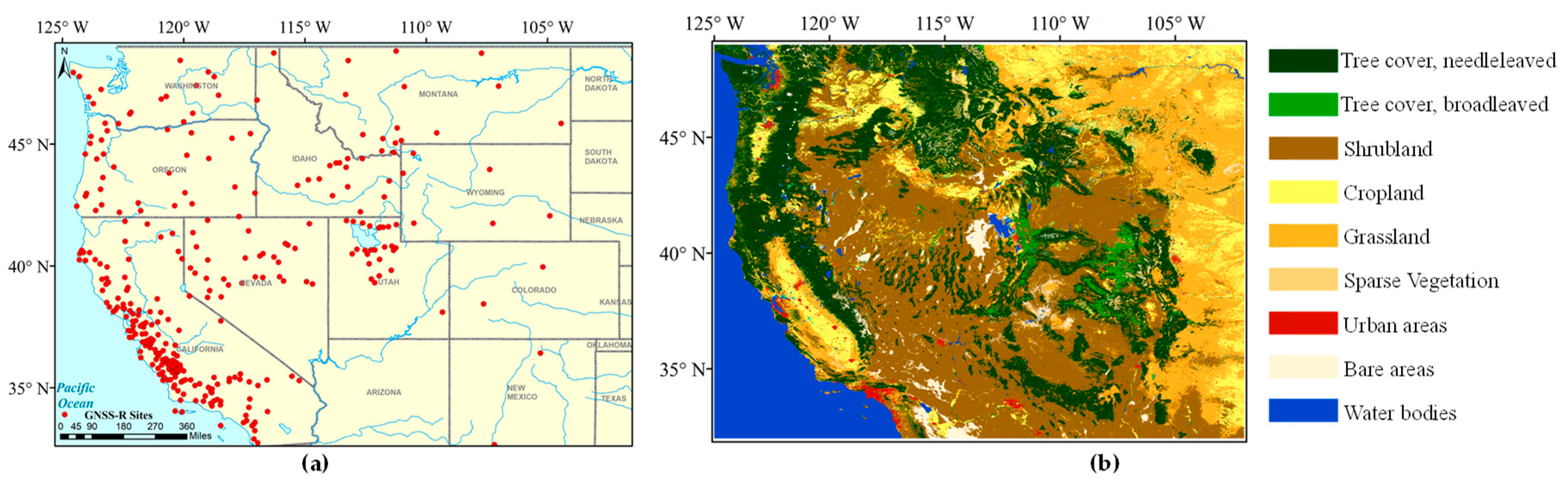
2.1. Study Area

The western part of the continental U.S. (CONUS) in the range of latitude and longitude between 32 °N–49 °N and 125 °W–102 °W was selected as the study area in this research (Figure 1), since nearly all the PBO H2O sites used for NMRI monitoring are distributed in this region. In addition, to the best of our knowledge, the PBO H2O network in the west of the CONUS is the only operational network based on the GNSS-IR principle to produce archived and publicly available vegetation information products. Meanwhile, serious drought events occurred in this region during 2012–2014, and VWC is recognized as a key indicator for drought monitoring and prediction. This can provide a validation method for us to evaluate the fusion results through the drought events.
Large areas of land cover in the western part of the CONUS consist of low vegetation types, such as shrubland, grassland, and cropland, except the regions in the western of Washington, Oregon along the Pacific Ocean, and central and eastern part of Idaho, where the main topography is mountain dominated by tree cover (Figure 1b). The land cover map is from the European Space Agency Climate Change Initiative (ESACCI) project (http://maps.elie.ucl.ac.be/CCI/viewer/index.php) [37,38]. The climate of the study area is known to be arid to semi-arid with three typical climate types: the temperate oceanic climate, Mediterranean climate, and plateau mountain climate [39]. The oceanic climate along the Pacific coast is warm in winter and cool in summer, with abundant rainfall. The dry climate of the western plateau is an inland climate, and the annual temperature difference of the plateau area is large. The Mediterranean climate is characterized as mild and wet in winter and warm and dry in summer [40].

2.2. Data Resources

2.2.1. The Normalized Microwave Reflection Index (NMRI)

The NMRI was first proposed by Larson and Small [21]. NMRI is an index reflecting the change of VWC estimated from data archived by GNSS instruments deployed for geodetic applications. GNSS satellites transmit L-band microwave signals, and some of this energy is reflected by the surface surrounding the antenna, which causes the multipath effect. Then, the GPS receivers receive the interference signal of the direct signal and reflected signal. The VWC variation can be estimated by the GNSS-IR system, since the multipath effect of GNSS satellites changes due to the existence of vegetation cover on the ground, as the amplitude of the GPS interferometric signal varies with the change of VWC. Based on this, the NMRI is defined, which increases as VWC increases. For the principle of the GNSS-IR technique and the detailed calculation process of NMRI, we refer the readers to the Appendix A. Furthermore, the NMRI was validated at four sites in Montana, and the results showed that the NMRI is correlated strongly with VWC and NDVI [33]. Recently, the NMRI was also used to evaluate the vegetation response to a recent drought in California, U.S., and was compared with the optical-based remote sensing NDVI [40].
The NMRI data used in this study were obtained from the PBO H2O Data Portal (https://gnss-h2o.jpl.nasa.gov/index.php) [41], which up to now is the only operational network based on the GNSS-IR principle to produce archived and publicly available vegetation information products. There are 329 PBO H2O sites that meet the requirements within the study area, as shown in Figure 1a. At the locations of these PBO H2O sites, the types of land cover include shrubland, cropland, grassland, and savanna. The study period is from January 1, 2007, to December 31, 2016. The daily NMRI data can be obtained for each site.

2.2.2. Indices Related to the VWC
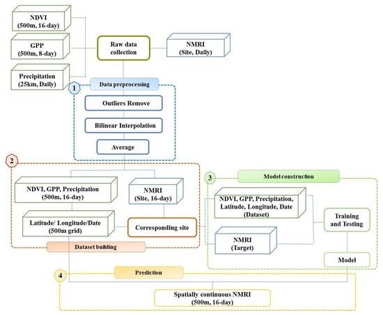
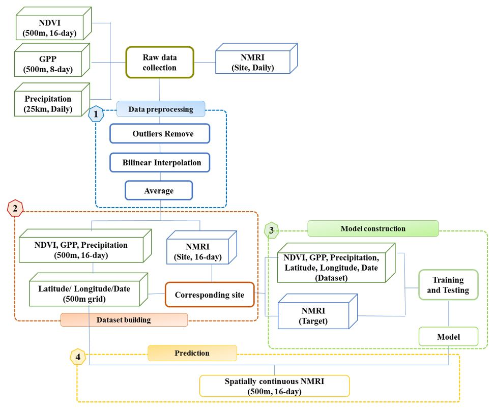
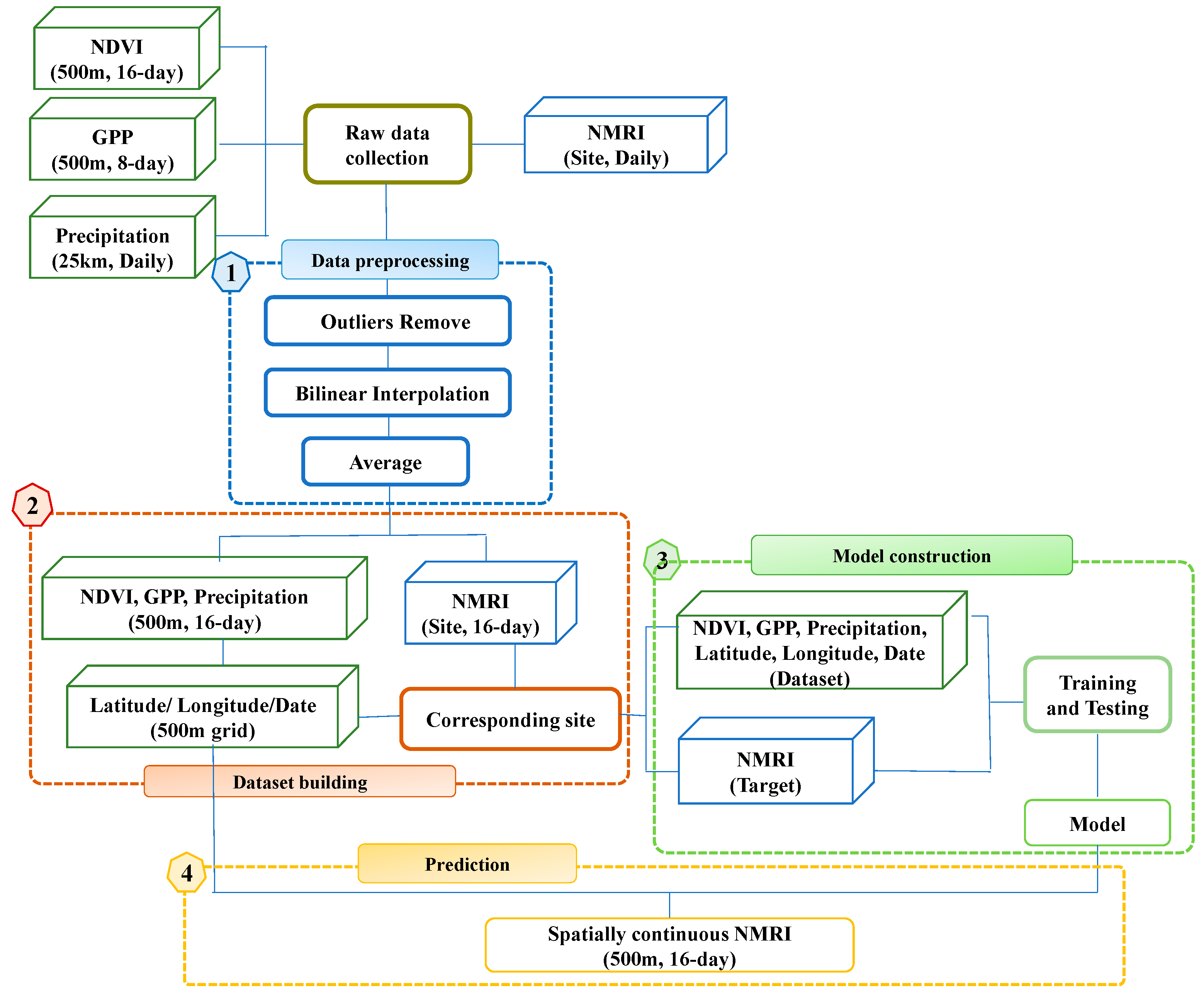
In this paper, six indices related to VWC in biological and meteorological mechanisms, i.e., NDVI, NDWI, NDII, gross primary productivity (GPP) [42], leaf area index (LAI) [43], and precipitation are used to evaluate their potentiality as auxiliary datasets through correlation analysis [6,44,45].
NDVI, representing greenness, is computed from the Moderate Resolution Imaging Spectroradiometer (MODIS) reflectance in the Red and NIR bands. GPP refers to the total organic carbon fixed by photosynthesis in unit time and area, including autotrophic breathing and heterotrophic breathing. LAI refers to the ratio of total leaf area to land area, representing the density of vegetation. NDWI and NDII, representing water content, are calculated from the MODIS reflectance in the Red and SWIR1 (SWIR2) bands. All the vegetation indices mentioned above can be downloaded from the NASA Land Processes Distributed Active Archive Center (LP DAAC) (http://ladsweb.nascom.nasa.gov). The specific products used in this study are listed in Table 1.
Precipitation is a very important meteorological parameter for the understanding of land surface processes and global climate change and plays a key role in the growth of vegetation. Therefore, we also added the precipitation variable into the experimental process. The TRMM_3B42RT_Daily product produced by the NASA GES DISC was chosen for the analysis [46]. We analyzed these potential indices related to VWC in Section 3.1 and Section 4.1 in details to determine the model input.

3. Methodology

The objective of the proposed method is to obtain spatially continuous NMRI products by fusing optical remote sensing VWC-related indices. Specific process of the point–surface fusion model used in this study is described below, and a flowchart of the method is shown in Figure 2.
(1)Data processing and dataset selection. Firstly, we removed outliers from the dataset and unified the temporal and spatial resolutions to 16 days and 500 m. Then, we analyzed the correlation between the variables and select the best auxiliary dataset.
(2)Dataset building. We identified all the NDVI, GPP, and precipitation data corresponding to the longitude and latitude coordinates of NMRI at the PBO H2O sites, and the dataset was built with NDVI, GPP, and precipitation, along with longitude, latitude, and date.
(3)Model construction. With the dataset constructed as input, the corresponding NMRI values were used as targets. Machine learning models were built, and a 10-fold cross-validation method was used to validate the effectiveness of the models.
(4)Prediction. VWC-related indices of the grids were used as the input to the models. A spatially continuous 500 m NMRI product was obtained, and VWC information, where PBO H2O sites are not located, could be acquired.

3.1. Data Processing and Dataset Selection

An NDVI less than 0 and GPP (LAI) greater than 30,000 (248) are removed to eliminate the effects of ice- and snow-covered areas, water bodies, buildings, and other features. (The thresholds are based on the Product User’s Guide provided by NDVI, GPP, and LAI data source website, http://ladsweb.nascom.nasa.gov).
To uniformize the temporal resolution, all datasets are averaged to 16 days. Because the spatial resolution of precipitation is different from other auxiliary data, the precipitation product with a spatial resolution of 25 km is resampled to 500 m by the nearest neighbor interpolation method based on the assumption that the precipitation is the same within a certain range. For each GPS site, the auxiliary variable value corresponding to the longitude and latitude of NMRI is extracted from the image. The data pairs of NMRI, and the auxiliary variables of 329 sites for 10 years, are obtained.
The approach of auxiliary datasets selection is based on correlation analysis. Firstly, for every vegetation type, a long time series variation between NMRI and auxiliary variables over the ten years from 2007 to 2016 are analyzed to verify the covariance between them. Then, for each site, the Pearson correlation coefficient (R) between each auxiliary variable and NMRI is calculated. Meanwhile, the R among the auxiliary variable for all the 329 sites is counted to eliminate the redundancy of datasets. Finally, the dataset is selected based on the following main requirements: (1) physical and chemical significance for the change of VWC. (2) a strong correlation with NMRI; (3) reduced data redundancy. The detailed discussion of the correlation analysis can be found in Section 4.1.

3.2. Machine Learning Methods

3.2.1. Back-Propagation Neural Network (BPNN)

The BPNN is the most common neural network algorithm. It is simply a gradient descent method designed to minimize the total error (or mean error) of the output computed by the network. It has the advantage of good self-adaptation, self-learning, robustness, and generalization. Therefore, the BPNN has been widely used in many fields, such as function approximation, regression, image processing, pattern recognition, and so on [47]. There is always one input layer, one output layer, and at least one hidden layer in the network. The regression model is trained with the use of forward propagation and backward propagation. Finally, the prediction samples are input into the trained network, and the final prediction results are obtained.

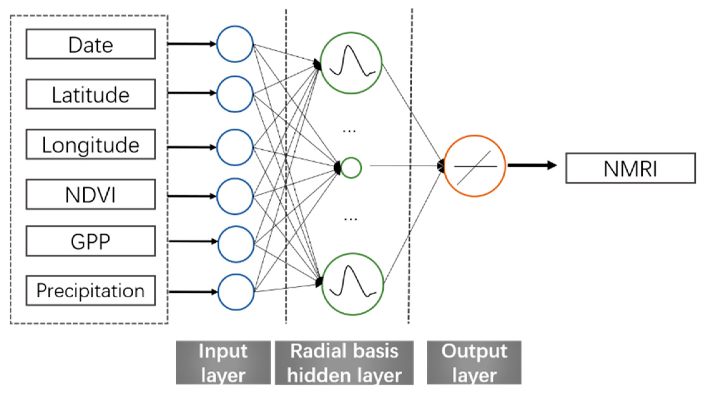
3.2.2. Generalized Regression Neural Network (GRNN)

The BPNN is a well-known neural network algorithm. However, it has the disadvantages of slow convergence and easily convergence to local minima. Another neural network, the GRNN, which is a special form of a radial basis function neural network, was proposed by Specht [40]. The GRNN improves the local approximation ability and learning speed, because the hidden nodes of the GRNN are often connected by a Gaussian function, which is locally distributed and attenuated to the center of the radial symmetry [48]. Meanwhile, compared with the popular feedforward neural networks, the GRNN has the advantages of a relatively simple structure, rapid training, low computational cost, and global convergence. GRNN contains three layers, i.e., an input layer, a radial basis hidden layer, and a special linear output layer. The input variables are transferred to the radial basis hidden layer from the input layer through a transfer function, which is always a Gaussian function. The output of the radial basis hidden layer is then not directly connected with the linear output layer but is first transmitted by a dot function and then connected to the output layer by the linear transfer function to calculate the network output. The structure of the GRNN algorithm is shown in Figure 3. In our study, the input signals are date, latitude, longitude, NDVI, GPP, and Precipitation, and the output parameter is NMRI. GRNN model is implemented by using the neural network toolbox of MATLAB.

3.2.3. Random Forest (RF)

The RF model was first proposed by Breiman [36]. The RF model is a nonlinear statistical ensemble bagging method that constructs and subsequently averages many randomized de-correlated decision trees for classification and regression purposes [49]. For a regression problem, RF is a flexible and practical method that has the following characteristics: (1) it is unexcelled in accuracy among the current algorithms, and runs efficiently on large databases; (2) it can handle thousands of input variables without variable deletion; (3) it generates an internal unbiased estimate of the generalization error as the forest building progresses; and (4) it features an effective method of estimating missing data and maintains accuracy when a large proportion of the data are missing. Based on the above advantages, the RF model has been widely used in the establishment of regression relations, and good prediction results have been obtained [50,51].
In regression, RF employs recursive partitioning to divide the data into many homogeneous subsets, and multivariate regression trees are built using a deterministic algorithm. The results of all the trees are then averaged. In each subset, each tree is independently grown to its maximum size based on a bootstrap sample from the training dataset, without any pruning, and the ensemble predicts the data that are not in the tree (the out-of-bag (OOB) data). The regression tree is built by selecting a random set of predictors (the dataset) and response variables (the target) by a set of decision rules. The rules are constructed based on recursively partitioning the input space into successively smaller regions, which are determined by binary splits. By calculating the difference in the mean-square error between the OOB data and the data used to grow the regression trees, the RF algorithm provides an error for the prediction called the OOB error of the estimate for each variable. The binary splits in the feature space are then selected by minimizing the difference in a cost function, between the response variable and the predicted response that would result from a specific split. The final output is the model in the form of a tree, with the branches corresponding to the splitting rules and terminal nodes corresponding to the mean response for a particular set of decision rules [49]. In our study, the RF model is implemented based on the package compiled with MATLAB and Visual C++ express edition, downloaded from Google code (https://code.google.com/archive/p/randomforest-matlab/downloads).

3.3. Traditional Multiple Linear Regression (MLR) Method for Comparison

The MLR algorithm is a common regression method. In this study, the relationship between NMRI and its corresponding NDVI, GPP, and precipitation was established by MLR:
NMRI = b0 + b1 × NDVI + b2 × GPP + b3 × Precip
where b0 is the intercept for NMRI prediction and b1–b3 are regression coefficients for the predictor variables, calculated by the least-squares method.

3.4. Validation Methods and Evaluation Indicators

In this paper, the 10-fold cross-validation method [52] is applied to verify the validity of the five point–surface fusion methods. The basic idea is to divide the original datasets randomly into 10 equal-sized parts. Nine parts are then used as the training set for model fitting, and the remaining part is used as the validation dataset for model testing. We then repeat the process 10 times so that every part is tested. Finally, the 10 results can be averaged to produce the final estimation called the “cross-validation results”, and the model with the maximum correlation coefficient is selected as the best fitting model for the later prediction. To verify the effectiveness of each model, the training sets and the test sets are quantitatively evaluated. The indicators are R and the RMSE.

4. Experiment and Analysis

4.1. Dataset Selection

Figure 4 shows the long time-series variation diagrams of the seven indices over the four vegetation types. For all four vegetation types, the general trend of NMRI is consistent with that of NDVI, and it shows obvious annual cycle variability with one peak. GPP and LAI have similar variation trends and are more consistent with NMRI. For NDWI and NDII, the annual variation cycle is obvious but different from that of NMRI with two peaks in each cycle. Then, we analyzed the correlation between NMRI and other VWC-related indices among the 329 sites during the 10 years, as shown in a statistical bar chart featuring the number of sites in different ranges of correlation coefficients (R) in a 10 year range and the statistical distribution box charts of the R among the 329 sites of each year (Figure 5). The distribution of the R in each year is about the same. For NDVI, the R of most of the sites is between 0.2 and 0.6. For NDWI and NDII, their correlation with NMRI is much lower than that of NDVI, with most of the sites concentrated in the range of 0 to 0.4. When it comes to GPP and LAI, the results are clearly different. The correlation between GPP (LAI) and NMRI is very high with R of most of the sites concentrated on 0.6–0.9 (0.5–0.8). However, R values between precipitation and NMRI are relatively low, between −0.4 and 0.4, and the distribution of positive and negative values is symmetrical.
Based on the above analysis, the conclusion can be drawn that the overall correlation between NMRI of GPP and LAI is the highest, NDVI is the second, NDWI and NDII are smaller still, and precipitation is the lowest. Then, to reduce data redundancy, we analyzed the correlation between the six VWC-related indices during the 10 years (Figure 6). It indicates that the correlation between GPP and LAI is particularly high, in that the R can reach 0.9. Finally, the ultimate fusion input datasets are formed by NDVI, GPP, and precipitation, along longitude, latitude, and date, considering requirements in Section 3.1. The longitude, latitude, and date were added to introduce temporal and spatial information. The NDWI and NDII were removed owing to their low correlation with NMRI. The meteorological factor precipitation was retained for the change of precipitation directly causes the change of soil moisture, which may have a lag effect on the growth of vegetation and the variation of VWC.

4.2. Performance of the Models

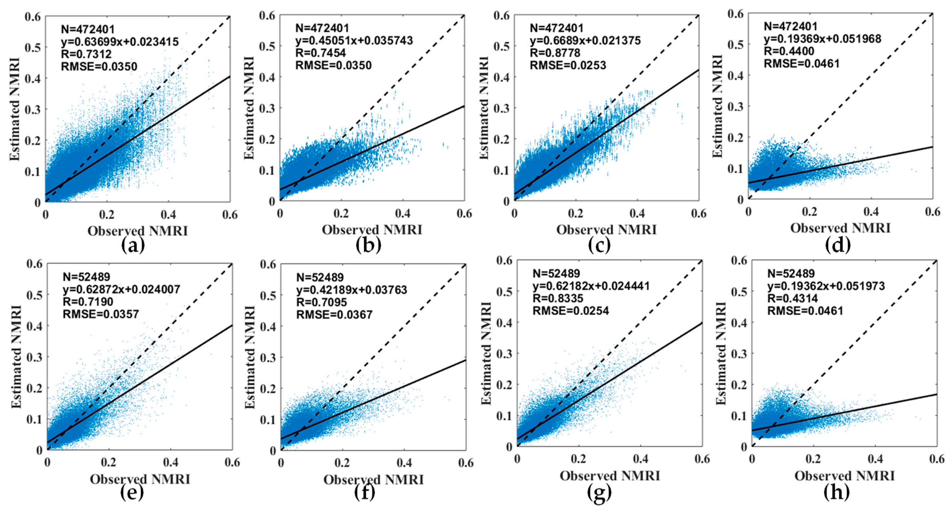
4.2.1. Overall Performance of the Models

Figure 7 shows the quantitative evaluation results and scatter diagrams of the 10-fold cross-validation performance of the three machine learning models compared with MLR. In model fitting, R values range from 0.44 to 0.88, and RMSEs from 0.25 to 0.46. In the cross-validation results, a similar trend appears with no obvious overfitting phenomenon, which proves the validity and applicability of the trained models. Compared to traditional MLR, the RMSE values of the machine learning methods are less than 0.037 and R values are greater than 0.7, but the R (RMSE) of MLR is only about 0.4 (0.046). The machine learning methods show obvious superiority, as they are better to simulate the complex nonlinear relationship and the hidden features within the datasets. When comparing the three machine learning methods, we find that RF performs the best, with the R of RF greater than 0.80 and the RMSE less than 0.03, followed by GRNN and BPNN. From the scatter diagrams, the models somewhat overestimate the NMRI when the NMRI values are low, and underestimate when the NMRI values are at a higher degree; this phenomenon is particularly evident in MLR. Among all the methods, the RF model obtains the best results, the point distribution is the densest near the fitting line, and the maximum slope is obtained. This is followed by BPNN and GRNN with a more dispersed scatter diagram. Similarly, the results of MLR are still the worst.

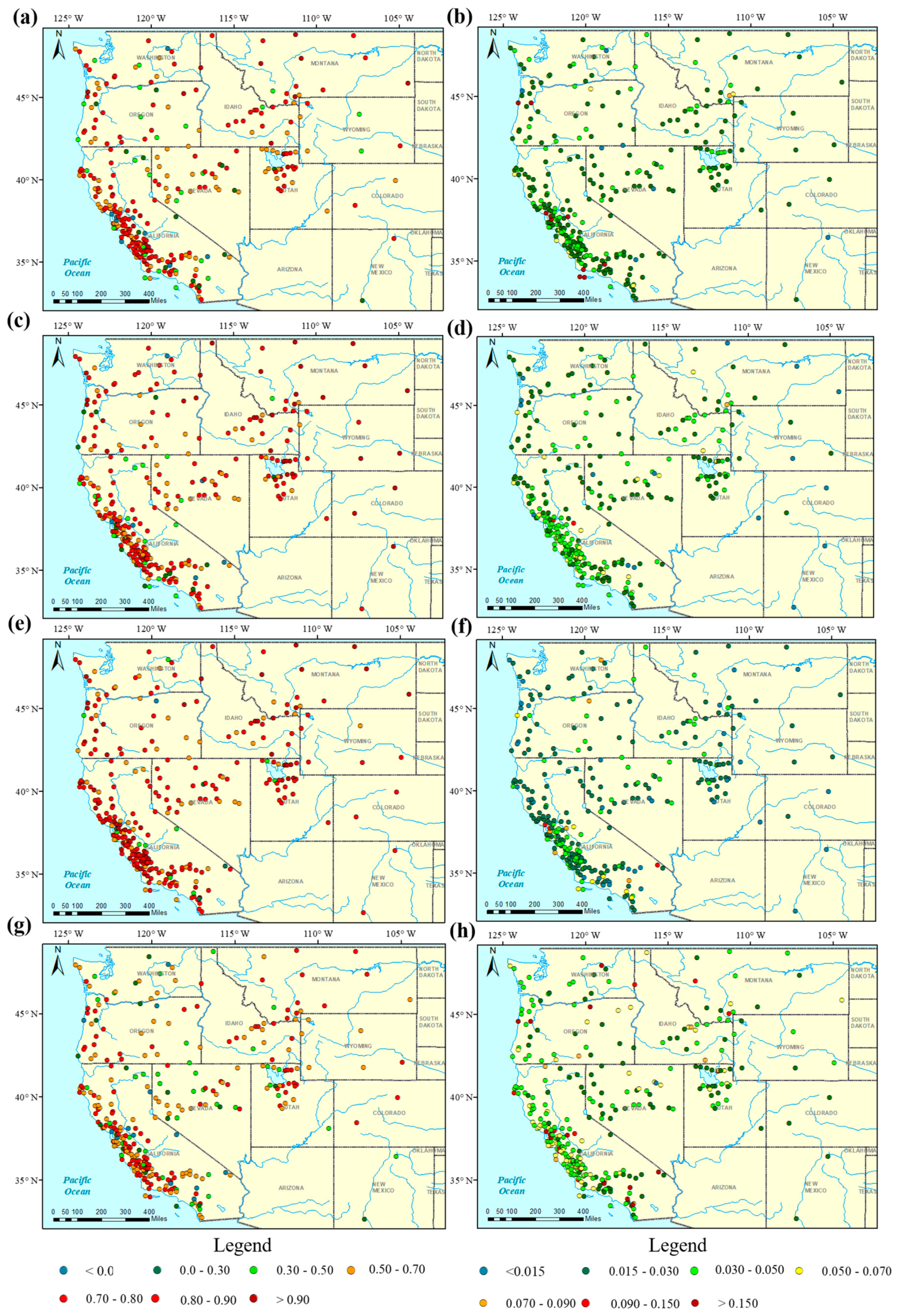
4.2.2. Model Performance for Each Site

To further analyze the spatial performance of the models, the R and RMSE values between the observed and estimated NMRI using these models over the 329 sites was calculated, and the results are presented in Figure 8. MLR has a significantly poor performance, with the R values of most sites lower than 0.7 and RMSE values higher than 0.03. The R values of 261 out of 329 sites for the RF model are greater than 0.7, and only 226 (203) out of 329 sites for the GRNN (BPNN) model are greater than 0.7. Meanwhile, 95% of the total sites report an RMSE of less than 0.03 for the RF model, and only 67% (55%) report an RMSE of less than 0.03 for BPNN (GRNN). This shows that, in terms of both R and RMSE, the RF results are superior to those of BPNN and GRNN in most sites. The randomness of RF, which is manifested in choosing observations at random and choosing features at random, makes the estimated results more robust. Comparing the two machine learning methods with relatively poor results, the sites where R values for BPNN are worse than those of GRNN are mainly concentrated in the eastern area with sparse site distribution, while the sites where RMSE values for BPNN are better than those of GRNN are mainly concentrated in the western coastal area, with dense site distribution. This is mainly due to the fact that BPNN has a disadvantage of easily converging to local minima, whereas GRNN improves the local approximation ability and has the advantage of global convergence. Therefore, GRNN is more stable and less sensitive to the density of site distribution than the BPNN.
Based on the comparison and analysis of the overall accuracy and the performance for each site with these models, we can summarize that the machine learning methods show an obvious superiority over the traditional linear fitting methods, and among the three machine learning methods, RF shows the best performance. BPNN and GRNN have slightly poor performance, and their overall performance is comparable.

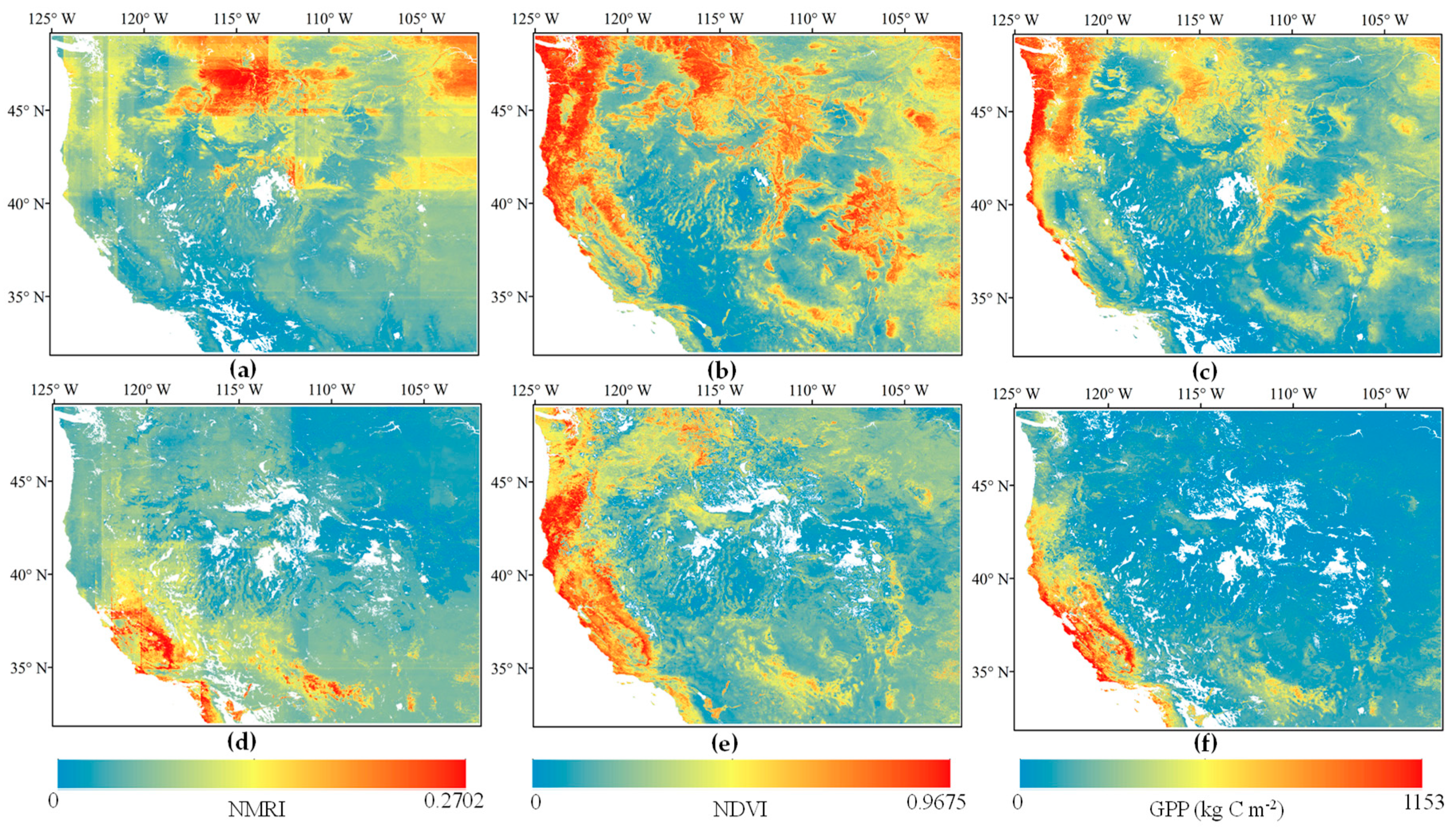
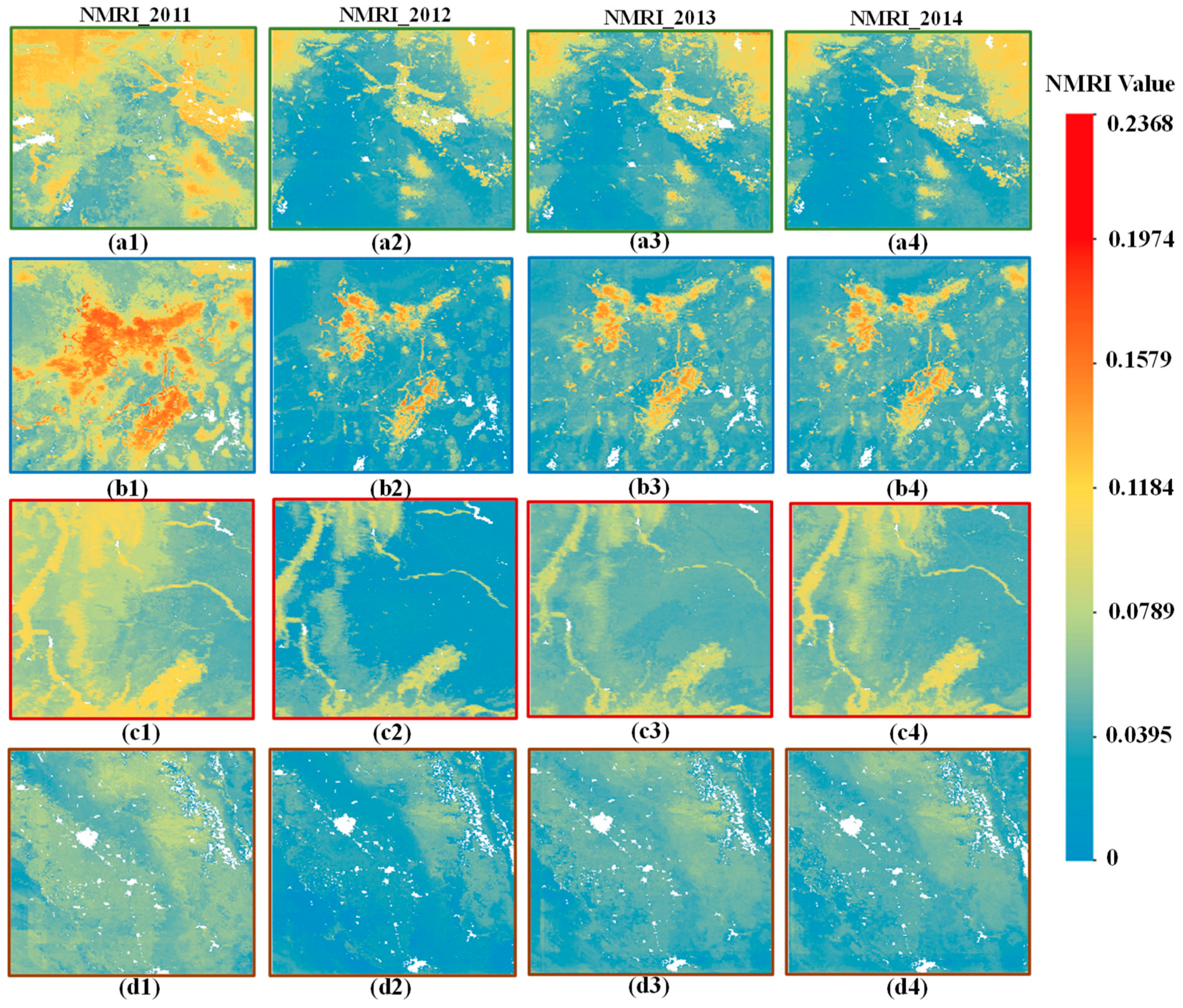
4.3. Point–Surface Fusion Results of NMRI

Owing to the good prediction ability of the RF model, a spatially continuous 500 m spatial resolution NMRI product was obtained. Figure 9 shows the fused NMRI map compared with the NDVI and GPP in summer and winter. The blank area in the map is unable to be retrieved because the auxiliary data has been removed for the effects of ice- and snow-covered areas, water bodies, buildings, and other features. In general, the spatial distributions of the NMRI are consistent with that of NDVI and GPP. That is, in summer, the three indices are reported to have higher values in the middle of the northern region and the north-east corner, whereas the southern region and the central inland region are lower. When it comes to the winter condition, the spatial distribution changes significantly, but the consistency between the three indices retains. Most areas in the central inland and north-east regions suffer a reduction of vegetation growth owing to the coming of winter. However, the vegetation in the areas of the California experience a growth, shown as all the three indices increased obviously in this region. This is mainly due to special climate of California, Mediterranean climate, which is characterized as dry, hot in summer and mild and wet in winter. Therefore, in summer the dry and hot climate will inhibit the vegetation growth, while in winter the suitable mild climate can bring a growing season to the vegetation [40]. The consistency of NMRI spatial distribution with NDVI and GPP further proves the accuracy of the point–surface fusion results.
However, there is still some inconsistency in the NMRI map, such as the higher NDVI and GPP values in the west of Washington and Oregon along the southern coastal alongside smaller NMRI values. One of the reasons could be that the vegetation type in this area is mainly tree cover, as shown in Figure 1b, while the PBO H2O network is always located in sites with low vegetation, like grassland, cropland, and shrubland. When the NMRI measured by the PBO network directly extends to forests with tree covers, the index may not be as applicable as before. Furthermore, although a small number of PBO H2O sites are also distributed in the forest area, they are usually located in open spaces 10 m away from the nearest trees in the forest. Because these GPS sites are originally designed for a position needed to reduce multipath effects [40]. Therefore, the current PBO sites are mainly designed to monitor the water content of nearby shrubs, herbs, mosses, and lichens, but NDVI and GPP products have a lower spatial resolution and usually measure the vegetation growth condition of all the green plants in the range, including trees, shrubs, and herbs. As a result, NMRI has some limitations in higher vegetation areas, which is shown as an underestimation of VWC information.
Meanwhile, there are still some shortcomings in the RF-based NMRI map, e.g., the blocky effect in Figure 9a,d, which affects the continuity of the whole picture. Such blocky effects have also been found in other regression studies using RF models [53,54]. This phenomenon is mainly due to the characteristics of the RF model. RF is a model based on a decision tree, which selects different features to judge the bifurcation and direction of the decision tree to obtain the final regression result. Therefore, when the range of the judgment conditions is broad and similar variables are input to the trained model, multiple distinct input variables can easily correspond to the same output variable, thus producing the blocky effect. In the point–surface fusion process, the grid data of latitude and longitude have the same interval and a fixed range, so it is easier for input variables with the same latitude and longitude to obtain the same prediction value, resulting in a blocky boundary similar to the distribution of the longitude and latitude in the fusion results. By analyzing the importance of the model variables, we find that, in the RF regression model, the importance of latitude and longitude ranks in the top three among all the predictive variables (Figure 10), indicating that the model is too sensitive to the longitude and latitude variables.
To conclude, although the blocky effect exists in the fusion results, the overall accuracy and the trends of spatial distribution of the results will not be affected. After fusing the site-level NMRI product and optical remote sensing VWC-related indices using machine learning methods, the spatial limitations of the original NMRI product can be compensated.

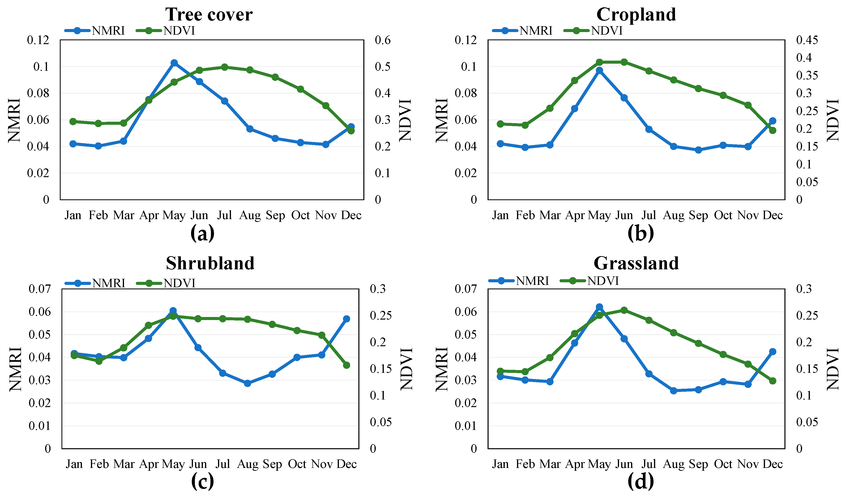
4.4. Long Time-Series Variation of NMRI and Drought Events

According to data released by the National Drought Mitigation Center (NDMC), two-thirds of the U.S. experienced a severe drought in 2012. This drought was the worst drought since the 1950s, which lasted three years and did not improve until 2015. The NDMC produces Vegetation Drought Index (VegDRI), a product that indicates the effect of drought on vegetation, in collaboration with the U.S. Geological Survey (USGS) Center for Earth Resources Observation and Science (EROS) and the High Plains Regional Climate Center (HPRCC) (https://www.drought.gov). Figure 11 shows the distribution of VegDRI in July for 2010–2016. The area marked by the red box is the research area of this paper.
We chose the worst drought year of 2012 to analyze the seasonal changes of VWC in the western part of the CONUS according to the monthly average NMRI and NDVI long time-series variation diagrams of four land cover types (Figure 12). Beginning in March, vegetation begins to grow with the approach of spring. From April to July, the NDVI values grow to their maximum, and then decrease with the arrival of autumn and winter. Compared with NDVI, the NMRI performs differently; it begins to increase in March and reaches the peak value at May, then it experiences a sharp decline owing to the severe drought in summer, since drought is especially severe in the summer because of the hot and dry climate in the western U.S. As a result, the NMRI index, which can reflect the VWC change information, is more sensitive than the NDVI index that only reflects a change in the greenness of the vegetation to the occurrence of a drought event. During the drought period from May to July, NMRI values for cropland, shrubland, and grassland decreased by 50%, while NMRI values for tree cover only reduced by 30%. This indicates that the high vegetation types are less affected by drought.
Then, we selected July with the worst drought to analyze the inter-annual variation of VWC in the western part of the CONUS over the decade from 2007 (Figure 13). When the severe drought in 2012 occurred, the water content of all vegetation types experienced a dip with NMRI fallen by 22% to 50%. NDVI has also experienced a reduction, but not as severe as NMRI (only about 4% to 16%). NMRI and NDVI were recovered and gradually became stable after the drought conditions were relieved. Similarly, the tree cover was least affected by drought, with NMRI decreasing by 30% and NDVI decreasing by only 4%. Identical results can be obtained from the previous drought spatial distribution map (Figure 11). In terms of drought spatial distribution, the regions with severe drought are mainly concentrated in the central inland region, where the main vegetation types are shrubland and grassland. Areas with higher vegetation suffer from a weaker drought. Therefore, we will focus on low-vegetation areas that are more sensitive to drought events in the following analysis.
Figure 14 selects the 500 m NMRI results in July from 2010 to 2016 as the basis for the analysis of the changes in VWC during the summer drought. During the non-drought period from 2010 to 2011, the NMRI was normal and higher in the west, north, and central/eastern regions. However, it is worth noting that there is a marked decrease for NMRI in 2012, especially in the southern part of the western coastal state of California, the southern part of Idaho, Northeastern Colorado, Northeast Utah, and Southwestern Wyoming. To analyze the NMRI variation more clearly, the enlarged NMRI maps in the above-mentioned areas of the four frames from 2011 to 2014 in Figure 14 are shown in Figure 15. In Figure 15a–d, the four sets of diagrams respectively represent the enlarged NMRI map in the four corresponding color boxes in Figure 12. When the severe drought occurred in 2012, most of the areas in Figure 15a2–d2 were reported to suffer a significant reduction in NMRI compared with the situation in 2011 with a relatively high level of NMRI. Possible reasons for the decline in NMRI and the drought event are climate conditions and vegetation types in these regions. California is a Mediterranean climate, which is dry and hot in summer; Wyoming is dry and always has little rain; Southern Idaho is dominated by a continental climate with less precipitation; and Northeast Utah has a slightly larger Salt Lake desert, with lower annual precipitation and a drier climate. These dry climates lead to a significant reduction in NMRI. Moreover, as shown in the land cover map in Figure 1b, the vegetation types where the most severe drought event occurred mainly consist of low vegetation, such as shrublands, grasslands, and croplands, which were proven to be more vulnerable to drought in Section 4.2. The situation was similar in 2013 and 2014, but not as severe as in 2012. By 2015, the drought was alleviated, and the NMRI rose, compared to the NMRI from 2012 to 2014, and then returned to the normal situation, as in 2011.
Based on the above experimental results, the consistency between the distribution map of NMRI and that of the drought index indicates that the NMRI shows a significant response to drought events. NMRI will, thus, be an effective measure to predict the location, occurrence, and duration of drought events and allow corresponding precautions to be made using relatively high-resolution spatially continuous NMRI products after point–surface fusion.

5. Conclusions and Future Research

In this study, we first analyzed the correlation between six VWC-related indices and the NMRI product, based on GNSS-IR. The three machine learning methods of BPNN, GRNN, and RF were used to construct point–surface fusion models using data from 2007 to 2016. The results showed that the machine learning methods outperformed the traditional methods of MLR in the cross-validation results. Among the three machine learning methods, the results of RF were the best, followed by those of GRNN and BPNN. Then, by using the RF model, we obtained an NMRI product with a spatial resolution of 500 m, which compensate for the spatial limitations of the NMRI product in the PBO H2O sites. Finally, maps of the 500 m spatial resolution NMRI product for the summer from 2010 to 2016 were obtained. The results showed that, during the period from 2012 to 2014, when drought occurred in the western part of the CONUS, the NMRI value was also significantly reduced, which is consistent with the drought distribution map. In conclusion, this paper proves the effectiveness of using machine learning methods to acquire the spatially continuous NMRI product with a point–surface fusion technique, and verifies the feasibility of analyzing and predicting drought events by using spatially continuous products with a finer resolution.
In the future, NMRI products can be fused with other VWC-related microwave remote sensing data to obtain an NMRI product with higher accuracy. Furthermore, other meteorological factors related to vegetation growth, such as LST, will be added into the model. Statistical distance approaches, such as the Jeffries Matusita distance [55,56,57,58], can be used to assess the statistical separability of variables and dataset selection. Other machine learning models, or deeper neural networks, will be used to study the relationship between NMRI and these vegetation indices, to further improve the accuracy of the model. Due to the fusion with optical remote sensing data, the temporal resolution of the final fusion result is limited by the optical remote sensing data. In our future work, we will consider the idea of combining point–surface fusion and spatial-temporal fusion to improve the temporal resolution of the NMRI products for the monitoring and prediction of more unexpected disaster events.

Author Contributions

Conceptualization, Q.Y.; Data curation, S.L.; Formal analysis, S.L.; Methodology, Q.Y. and S.L.; Resources, Q.Y. and T.L.; Supervision, L.Y., H.S. and L.Z.; Validation, S.L., L.Y., T.L., H.S. and L.Z.; Visualization, S.L. and L.Y.; Writing—original draft, S.L.; Writing—review & editing, Q.Y., L.Y., T.L., H.S. and L.Z.

Acknowledgments

This work was supported by the National Key R&D Program of China (No. 2016YFC0200900) in part of the Fundamental Research Funds for the Central Universities under Grant 2042019kf0213. Sincere thanks to anonymous reviewers and members of the editorial team, for the comments and contributions.

Conflicts of Interest

The authors declare no conflict of interest.

Appendix A. The Procedure to Calculate GNSS-IR Index NMRI.

Global Navigation Satellite System Interferometric Reflectometry (GNSS-IR) provides us with a new mode to monitor the vegetation information in a long time series. It acts as a relatively new L-band remote sensing technique with relevance for measuring vegetation states using reflected GNSS signals by recording the interference between a direct GNSS signal and a reflected GNSS signal [21].
L-band signals transmitted by GNSS satellites are reflected by the land surface and received by geodetic-quality GPS antennas a few meters above the ground. It causes the multipath effect and pseudorange multipath error (M) on the observations. It is found that the existence of vegetation has a certain effect on the amplitude of the interference between a direct GNSS signal and a reflected GNSS signal, as it decreases with the increase of vegetation water content. According to the definition and formula derivation based on M [59], M increases with the increase of the amplitude of the interference. This provides a possibility for the study of vegetation water content based on M.
Figure A1. Schematic diagram of monitoring vegetation water content by GNSS-IR.
Remotesensing 11 01440 g0a1
A database of daily mean MP1rms statistics for each site is routinely compiled by the operators of the NSF EarthScope Plate Boundary Observatory (PBO), based on which pseudorange multipath error (M) can be obtained. This original objective of this GPS network is to measure deformation across active fault zones in the western USA, and the network can also be used to monitor vegetation water content information according to the above theory. To eliminate the influence on topography and get a positive-correlation index with the vegetation water content, the index NMRI was obtained by normalization of MP1rms:
N M R I = ( M P 1 r m s max ( M P 1 r m s ) ) max ( M P 1 r m s )
The maximum MP1rms (shown by the dashed line) is based on the average of the largest 5% daily MP1rms values. Finally, the index NMRI is defined, which increases as vegetation water content increases. The lowest NMRI values (bottom 5% of the observed values) are set to zero; the peak values rarely exceed 0.35.

References

  1. Zhang, C.; Pattey, E.; Liu, J.; Cai, H.; Shang, J.; Dong, T. Retrieving Leaf and Canopy Water Content of Winter Wheat using Vegetation Water Indices. IEEE J. Stars 2017, 99, 1–15. [Google Scholar] [CrossRef]
  2. Zhang, J.H.; Xu, Y.; Yao, F.M.; Wang, P.J.; Guo, W.J.; Li, L. Advances in estimation methods of vegetation water content based on optical remote sensing techniques. Sci. China Technol. Sci. 2010, 53, 1159–1167. [Google Scholar] [CrossRef]
  3. Holzman, M.E.; Carmona, F.; Rivas, R.; Niclòs, R. Early assessment of crop yield from remotely sensed water stress and solar radiation data. ISPRS J. Photogramm. Remote Sens. 2018, 45, 297–308. [Google Scholar] [CrossRef]
  4. Rud, R.; Cohen, Y.; Alchanatis, V.; Levi, A.; Brikman, R.; Shenderey, C. Crop water stress index derived from multi-year ground and aerial thermal images as an indicator of potato water status. Precis. Agric. 2014, 15, 273–289. [Google Scholar] [CrossRef]
  5. Wang, Y.; Yuan, Q.; Li, T.; Shen, H.; Zheng, L.; Zhang, L. Evaluation and comparison of MODIS Collection 6.1 aerosol optical depth against AERONET over regions in China with multifarious underlying surfaces. Atmos. Environ. 2019, 200, 280–301. [Google Scholar] [CrossRef]
  6. Chuvieco, E.; Riaño, D.; Aguado, I.; Cocero, D. Estimation of fuel moisture content from multitemporal analysis of Landsat Thematic Mapper reflectance. Int. J. Remote Sens. 2002, 23, 2145–2162. [Google Scholar] [CrossRef]
  7. Jackson, R.D. Remote sensing of biotic and abiotic plant stress. Annu. Rev. Phytopathol. 2003, 24, 265–287. [Google Scholar] [CrossRef]
  8. Zhang, J.; Guo, W. Quantitative retrieval of crop water content under different soil moistures levels. Proc. SPIE 2006, 6411, 64110D. [Google Scholar]
  9. Gao, B.C. NDWI—A normalized difference water index for remote sensing of vegetation liquid water from space. Remote Sens. Environ. 1996, 58, 257–266. [Google Scholar] [CrossRef]
  10. Hardisky, M.A.; Lemas, V.; Smart, R.M. The influence of soil salinity, growth form, and leaf moisture on the spectral radiance of spartina alterniflora canopies. Photogramm. Eng. Rem. Sens. 1983, 49, 77–84. [Google Scholar]
  11. Zarco-Tejada, P.J.; Rueda, C.A.; Ustin, S.L. Water content estimation in vegetation with MODIS reflectance data and model inversion methods. Remote Sens. Environ. 2003, 85, 109–124. [Google Scholar] [CrossRef]
  12. Ceccato, P.; Gobron, N.; Flasse, S.; Pinty, B.; Tarantola, S. Designing a spectral index to estimate vegetation water content from remote sensing data: Part 1: Theoretical approach. Remote Sens. Environ. 2002, 82, 188–197. [Google Scholar] [CrossRef]
  13. Brakke, T.W.; Kanemasu, E.T.; Steiner, J.L.; Ulaby, F.T.; Wilson, E. Microwave radar response to canopy moisture, leaf-area index, and dry weight of wheat, corn, and sorghum. Remote Sens. Environ. 1981, 11, 207–220. [Google Scholar] [CrossRef]
  14. Kim, Y.; Jackson, T.; Bindlish, R.; Lee, H.; Hong, S. Radar Vegetation Index for Estimating the Vegetation Water Content of Rice and Soybean. IEEE Geosci. Remote Sens Lett. 2012, 9, 564–568. [Google Scholar]
  15. Srivastava, P.K.; O’Neill, P.; Cosh, M.; Lang, R.; Joseph, A. Evaluation of radar vegetation indices for vegetation water content estimation using data from a ground-based SMAP simulator. In Proceedings of the IEEE. Geoscience and Remote Sensing Symposium, Milan, Italy, 26–31 July 2015; pp. 1296–1299. [Google Scholar]
  16. Calvet, J.C.; Wigneron, J.P.; Walker, J.; Karbou, F.; Chanzy, A.; Albergel, C. Sensitivity of Passive Microwave Observations to Soil Moisture and Vegetation Water Content: L-Band to W-Band. IEEE Trans. Geosci. Remote Sens. 2011, 49, 1190–1199. [Google Scholar] [CrossRef]
  17. Liu, Y.Y.; De Jeu, R.A.M.; McCabe, M.F.; Evans, J.P.; van Dijk, A. Global long-term passive microwave satellite-based retrievals of vegetation optical depth. Geophys. Res. Lett. 2011, 38, L18402. [Google Scholar] [CrossRef]
  18. Entekhabi, D.; Njoku, E.; O‘Neill P., O.; Michael, S.; Jackson, T.; Entin, J.; Im, E.; Kellogg, K. The Soil Moisture Active Passive (SMAP) Mission. Proc. IEEE 2009. [Google Scholar] [CrossRef]
  19. Dasgupta, S.; Qu, J.J. Combining MODIS and AMSR-E-based vegetation moisture retrievals for improved fire risk monitoring. Proc. SPIE 2006, 6298. [Google Scholar] [CrossRef]
  20. Wang, Q.; Chai, L.; Zhao, S.; Zhang, Z. Gravimetric Vegetation Water Content Estimation for Corn Using L-Band Bi-Angular, Dual-Polarized Brightness Temperatures and Leaf Area Index. Remote Sens. 2015, 7, 10543–10561. [Google Scholar] [CrossRef] [Green Version]
  21. Larson, K.M.; Small, E.E. Normalized Microwave Reflection Index, I: A Vegetation Measurement Derived from GPS Data. IEEE J. Sel. Top. Appl. Earth Obs. Remote Sens. 2014, 7, 1501–1511. [Google Scholar] [CrossRef]
  22. Martin-Neira, M. A Passive reflectometry and interferometry system (PARIS) application to ocean altimetry. ESA J. 1993, 17, 331–355. [Google Scholar]
  23. Masters, D.; Axelrad, P.; Katzberg, S. Initial results of land-reflected GPS bistatic radar measurements in SMEX02. Remote Sens. Environ. 2004, 92, 507–520. [Google Scholar] [CrossRef]
  24. Garrison, J.L.; Komjathy, A.; Zavorotny, V.U.; Katzberg, S.J. Wind speed measurement using forward scattered GPS signals. IEEE Trans. Geosci. Remote Sens. 2002, 40, 50–65. [Google Scholar] [CrossRef] [Green Version]
  25. Komjathy, A.; Maslanik, J.; Zavorotny, V.U.; Axelrad, P. Sea ice remote sensing using surface reflected GPS signals. Geoscience and Remote Sensing Symposium. Proc. IGARSS 2000, 7, 2855–2857. [Google Scholar]
  26. Semmling, A.M.; Beyerle, G.; Stosius, R.; Dick, G.; Wickert, J.; Fabra, F.; Cardellach, E.; Ribó, S.; Rius, A.; Helm, A.; et al. Detection of arctic ocean tides using interferometric GNSS-R signals. Geophys. Res. Lett. 2011, 38, 155–170. [Google Scholar] [CrossRef]
  27. Larson, K.M.; Ray, R.D.; Nievinski, F.G.; Freymueller, J.T. The Accidental Tide Gauge: A Case Study of GPS Reflections from Kachemak Bay, Alaska. IEEE Geosci. Remote Sens. Lett. 2013, 10, 1200–1204. [Google Scholar] [CrossRef]
  28. Cardellach, E.; Fabra, F.; Rius, A.; Pettinato, S.; D’Addio, S. Characterization of Dry-snow Sub-structure using GNSS Reflected Signals. Remote Sens. Environ. 2012, 124, 122–134. [Google Scholar] [CrossRef]
  29. Rodriguez-Alvarez, N.; Bosch-Lluis, X.; Camps, A.; Aguasca, A.; Vall-Llossera, M.; Valencia, E.; Ramos-Perez, I. Review of crop growth and soil moisture monitoring from a ground-based instrument implementing the Interference Pattern GNSS-R technique. Radio Sci. 2011, 46. [Google Scholar] [CrossRef]
  30. Rodriguez-Alvarez, N.; Camps, A.; Vall-Llossera, M.; Bosch-Lluis, X.; Monerris, A.; Ramos-Perez, I.; Valencia, E.; Marchan-Hernandez, J.F.; Martinez-Fernandez, J.; Baroncini-Turricchia, G.; et al. Land Geophysical Parameters Retrieval Using the Interference Pattern GNSS-R Technique. IEEE Trans. Geosci. Rem. Sens. 2011, 49, 71–84. [Google Scholar] [CrossRef]
  31. Egido, A.; Caparrini, M.; Ruffini, G.; Paloscia, S.; Guerriero, L.; Pierdicca, N.; Floury, N. Global Navigation Satellite System Reflectometry as a Remote Sensing Tool for Agriculture. Remote Sens. 2012, 4, 2356–2372. [Google Scholar] [CrossRef]
  32. Wan, W.; Larson, K.M.; Small, E.E.; Chew, C.C.; Braun, J.J. Using geodetic GPS receivers to measure vegetation water content. GPS Solut. 2015, 19, 237–248. [Google Scholar] [CrossRef]
  33. Small, E.E.; Larson, K.M.; Smith, W. Normalized Microwave Reflection Index, II: Validation of Vegetation Water Content Estimates at Montana Grasslands. IEEE J. Sel. Top. Appl. Earth Obs. Remote Sens. 2014, 7, 1512–1521. [Google Scholar] [CrossRef]
  34. Rumelhart, D.E.; Hinton, G.E.; Williams, R.J. Learning Representations by Back Propagating Errors. Nature 1986, 323, 533–536. [Google Scholar] [CrossRef]
  35. Specht, D.F. A general regression neural network. IEEE Trans. Neural Netw. 1991, 2, 568–576. [Google Scholar] [CrossRef] [PubMed]
  36. Breiman, L. Random Forests. Mach. Learn. 2001, 45, 5–32. [Google Scholar] [CrossRef] [Green Version]
  37. European Space Agency (ESA). CCI Land Cover Product User Guide Version 2.4. ESA CCI LC Project, 2014. Available online: http://maps.elie.ucl.ac.be/CCI/viewer/index.php (accessed on 17 June 2019).
  38. Bontemps, S.; Herold, M.; Kooistra, L.; van Groenestijn, A.; Hartley, A.; Arino, O.; Moreau, I.; Defourny, P. Revisiting land cover observation to address the needs of the climate modeling community. Biogeosciences 2012, 9, 2145–2157. [Google Scholar] [CrossRef] [Green Version]
  39. Xu, H.; Yuan, Q.; Li, T.; Shen, H.; Zhang, L.; Jiang, H. Quality Improvement of Satellite Soil Moisture Products by Fusing with In-Situ Measurements and GNSS-R Estimates in the Western Continental U.S. Remote Sens. 2018, 10, 1351. [Google Scholar] [CrossRef]
  40. Small, E.E.; Roesler, C.J.; Larson, K.M. Vegetation Response to the 2012–2014 California Drought from GPS and Optical Measurements. Remote Sens. 2018, 10, 630. [Google Scholar] [CrossRef]
  41. The NASA Land Processes Distributed Active Archive Center (LP DAAC). Available online: https://lpdaac.usgs.gov/ (accessed on 11 October 2016).
  42. Melillo, J.M.; Mcguire, A.D.; Kicklighter, D.W.; Moore, B.; Vorosmarty, C.J.; Schloss, A.L. Global Climate-Change and Terrestrial Net Primary Production. Nature 1993, 363, 234–240. [Google Scholar] [CrossRef]
  43. Watson, D.J. Comparative Physiological Studies on the Growth of Field Crops: I. Variation in Net Assimilation Rate and Leaf Area between Species and Varieties, and within and between Years. Ann. Bot. 1947, 11, 41–76. [Google Scholar] [CrossRef]
  44. Shishi, L.; Chadwick, O.A.; Roberts, D.A.; Still, C.J. Relationships between GPP, Satellite Measures of Greenness and Canopy Water Content with Soil Moisture in Mediterranean-Climate Grassland and Oak Savanna. Appl. Environ. Soil Sci. 2011, 2011, 1–14. [Google Scholar]
  45. Hunt, E.R., Jr.; Qu, J.; Hao, X.; Wang, L. Remote sensing of canopy water content: Scaling from leaf data to MODIS. Proc. SPIE 2009, 7454, 745409. [Google Scholar]
  46. Goddard Earth Sciences Data and Information Services Center. TRMM (TMPA-RT) Near Real-Time Precipitation L3 1 day 0.25 degree × 0.25 degree V7. Savtchenko, A., Greenbelt, M.D., Eds.; Goddard Earth Sciences Data and Information Services Center (GES DISC). Available online: https://disc.gsfc.nasa.gov/datasets/TRMM_3B42RT_Daily_V7/summary?keywords=TRMM_3B42RT_Daily (accessed on 17 June 2019).
  47. Ding, S.; Su, C.; Yu, J. An optimizing BP neural network algorithm based on genetic algorithm. Artif. Intell. Rev. 2011, 36, 153–162. [Google Scholar] [CrossRef]
  48. Li, T.; Shen, H.; Zeng, C.; Yuan, Q.; Zhang, L. Point-surface fusion of station measurements and satellite observations for mapping PM 2.5, distribution in China: Methods and Assessment. Atmos. Environ. 2017, 152, 477–489. [Google Scholar] [CrossRef]
  49. Hutengs, C.; Vohland, M. Downscaling land surface temperatures at regional scales with random forest regression. Remote Sens. Environ. 2016, 178, 127–141. [Google Scholar] [CrossRef]
  50. Yang, R.; Zhang, G.; Liu, F.; Lu, Y.; Yang, F.; Yang, F.; Yang, M.; Zhao, Y.; Li, D. Comparison of boosted regression tree and random forest models for mapping topsoil organic carbon concentration in an alpine ecosystem. Ecol. Indic. 2016, 60, 870–878. [Google Scholar] [CrossRef]
  51. Were, K.; Bui, D.T.; Dick Øystein, B.; Singh, B.R. A comparative assessment of support vector regression, artificial neural networks, and random forests for predicting and mapping soil organic carbon stocks across an afromontane landscape. Ecol. Indic. 2015, 52, 394–403. [Google Scholar] [CrossRef]
  52. Rodríguez, J.D.; Pérez, A.; Lozano, J.A. S Sensitivity analysis of k-Fold Cross validation in prediction error estimation. IEEE Trans. Patt. Anal. Mach. Intell. 2010, 32, 569–575. [Google Scholar] [CrossRef]
  53. Zhao, X.; Jing, W.; Zhang, P. Mapping Fine Spatial Resolution Precipitation from TRMM Precipitation Datasets Using an Ensemble Learning Method and MODIS Optical Products in China. Sustainability 2017, 9, 1912. [Google Scholar] [CrossRef]
  54. Shi, Y.; Song, L. Spatial Downscaling of Monthly TRMM Precipitation Based on EVI and Other Geospatial Variables Over the Tibetan Plateau From 2001 to 2012. Mt. Res. Dev. 2015, 35. [Google Scholar] [CrossRef]
  55. Wang, Y.; Qi, Q.; Liu, Y. Unsupervised Segmentation Evaluation Using Area-Weighted Variance and Jeffries-Matusita Distance for Remote Sensing Images. Remote Sens. 2018, 10, 1193. [Google Scholar] [CrossRef]
  56. Zeng, W.; Lin, H.; Yan, E.; Jiang, Q.; Lu, H.; Wu, S. Optimal selection of remote sensing feature variables for land cover classification. In Proceedings of the Fifth International Workshop on Earth Observation and Remote Sensing Applications (EORSA), Xi’an, China, 18–20 June 2018; pp. 1–5. [Google Scholar]
  57. Novelli, A.; Tarantino, E.; Caradonna, G.; Apollonio, C.; Balacco, G.; Piccinni, F. Improving the ANN classification accuracy of landsat data through spectral indices and linear transformations (PCA and TCT) aimed at LU/LC monitoring of a river basin. In Proceedings of the International Conference on Computational Science and Its Applications, Ho Chi Minh City, Vietnam, 24–27 June 2017; pp. 420–432. [Google Scholar]
  58. Jia, Y.; Ge, Y.; Ling, F.; Guo, X.; Wang, J.; Wang, L.; Chen, Y.; Li, X. Urban Land Use Mapping by Combining Remote Sensing Imagery and Mobile Phone Positioning Data. Remote Sens. 2018, 10, 446. [Google Scholar] [CrossRef]
  59. Braasch, M.S. Multipath Effects. In Global Positioning System: Theory and Applications; Parkinson, B.W., Spilker, J.J., Jr., Axelrad, P., Enge, P., Eds.; the American Institute of Aeronautics and Astronautics: Reston, VA, USA, 1995; Volume 1, pp. 547–568. [Google Scholar]
Figure 1. Study area in the western part of the CONUS. (a) Study area and PBO H2O sites (https://gnss-h2o.jpl.nasa.gov/index.php). (b) Land cover map in 2015 (http://maps.elie.ucl.ac.be/CCI/viewer/index.php).
Remotesensing 11 01440 g001
Figure 2. Flowchart of the point–surface fusion model used in this study.
Remotesensing 11 01440 g002
Figure 3. Structure of Generalized Regression Neural Network (GRNN).
Remotesensing 11 01440 g003
Figure 4. The long time-series variation diagrams of the seven indices over the four vegetation types: (a) Savannas; (b) cropland; (c) shrubland; (d) grassland.
Remotesensing 11 01440 g004
Figure 5. The bar charts and box charts of the correlation coefficients (R) between the six indices and NMRI: (a1f1) bar charts of the correlation coefficients between the indices and NMRI in the different regions during the 10 years; (a2f2) statistical distribution box charts of the correlation coefficients of each year and the total of the 10 years from 2007 to 2016.
Remotesensing 11 01440 g005
Figure 6. Statistical box chart of the correlation coefficients among the VWC-related indices.
Remotesensing 11 01440 g006
Figure 7. Scatter plots of the comparison model results: (a) BPNN-model fitting; (b) GRNN-model fitting; (c) RF-model fitting; (d) MLR-model fitting; (e) BPNN-cross-validation; (f) GRNN-cross-validation; (g) RF-cross-validation; (h) MLR-cross-validation. The dashed line is the 1:1 line. Footnote: BPNN (Back-Propagation Neural Network), GRNN (Generalized Regression Neural Network), RF (Random Forest), MLR (Multiple Linear Regression).
Remotesensing 11 01440 g007
Figure 8. Spatial distribution of R and RMSE between the observed and estimated NMRI over the PBO H2O sites for the four models: (a) BPNN-R; (b) BPNN-RMSE; (c) GRNN-R; (d) GRNN-RMSE; (e) RF-R; (f) RF-RMSE; (g) MLR-R; (h) MLR-RMSE.
Remotesensing 11 01440 g008
Figure 9. Point–surface fusion results of 500 m NMRI compared with NDVI and GPP: (a) NMRI-Summer; (b) NDVI-Summer; (c) GPP-Summer; (d) NMRI-Winter; (e) NDVI-Winter; (f) GPP-Winter.
Remotesensing 11 01440 g009
Figure 10. The importance of the predictors in the random forest (RF) model.
Remotesensing 11 01440 g010
Figure 11. Vegetation Drought Index (VegDRI) distribution map for 2010 to 2016. Taken from https://www.drought.gov.
Remotesensing 11 01440 g011
Figure 12. NMRI and NDVI long time-series variation diagrams of four Land cover types in 2012: (a) tree cover; (b) cropland; (c) shrubland; (d) grassland.
Remotesensing 11 01440 g012
Figure 13. NMRI and NDVI long time-series variation diagrams of the four land cover types in July from 2007 to 2016: (a) tree cover; (b) cropland; (c) shrubland; (d) grassland.
Remotesensing 11 01440 g013
Figure 14. 500 m NMRI maps in July from 2010 to 2016.
Remotesensing 11 01440 g014
Figure 15. 500 m enlarged NMRI results of the four frame areas in Figure 13, from 2011 to 2014.
Remotesensing 11 01440 g015
Table 1. Indices used in the study.
IndexResolutionProductPeriod
NMRI [37]Daily/site-basedPBO H2O2007.01.01–2016.12.31
NDVI [6]16 day/500 mMOD13A12007.01.01–2013.12.31
NDWI [9]8 day/500 mMOD09A1 (bands 2,5)2007.01.01–2013.12.31
NDII [10]8 day/500 mMOD09A1 (bands 2,6)2007.01.01–2013.12.31
GPP [42]8 day/500 mMOD17A2H2007.01.01–2013.12.31
LAI [43]8 day/500 mMCD15A2H2007.01.01–2013.12.31
Precipitation [46]Daily/25 kmTRMM_3B42RT_Daily2007.01.01–2013.12.31
Footnote: NMRI (Normalized Microwave Reflection Index), NDVI (Normalized Difference Vegetation Index), NDWI (Normalized Difference Water Index), NDII (Normalized Difference Infrared Index), GPP (gross primary productivity), LAI (leaf area index).

