Comparative Study on Variable Selection Approaches in Establishment of Remote Sensing Model for Forest Biomass Estimation

Abstract

In the field of quantitative remote sensing of forest biomass, a prominent phenomenon is the increasing number of explanatory variables. Then how to effectively select explanatory variables has become an important issue. Linear regression model is one of the commonly used remote sensing models. In the process of establishing the linear regression model, a vital step is to select explanatory variables. Focusing on variable selection and model stability, this paper conducts a comparative study on the performance of eight linear regression parameter estimation methods (Stepwise Regression Method (SR), Criterions Based on The Bayes Method (BIC), Criterions Based on The Bayes Method (AIC), Criterions Based on Prediction Error (Cp), Least Absolute Shrinkage and Selection Operator (Lasso), Adaptive Lasso, Smoothly Clipped Absolute Deviation (SCAD), Non-negative garrote (NNG)) in the subtropical forest biomass remote sensing model development. For the purpose of comparison, OLS and RR, are commonly used as methods with no variable selection ability, and are also compared and discussed. The performance of five aspects are evaluated in this paper: (i) Determination coefficient, prediction error, model error, etc., (ii) significance test about the difference between determination coefficients, (iii) parameter stability, (iv) variable selection stability and (v) variable selection ability of the methods. All the results are obtained through a five ten-fold CV. Some evaluation indexes are calculated with or without degrees of freedom. The results show that BIC performs best in comprehensive evaluation, while NNG, Cp and AIC perform poorly as a whole. Other methods show a great difference in the performance on each index. SR has a strong capability in variable selection, although it is poor in commonly used indexes. The short-wave infrared band and the texture features derived from it are selected most frequently by various methods, indicating that these variables play an important role in forest biomass estimation. Some of the conclusions in this paper are likely to change as the study object changes. The ultimate goal of this paper is to introduce various model establishment methods with variable selection capability, so that we can have more choices when establishing similar models, and we can know how to select the most appropriate and effective method for specific problems.

1. Introduction

The importance of forest ecosystem services function has been universally acknowledged, especially in that it plays an important role in maintaining global carbon balance. Deforestation and conversion of forestland use types can cause carbon emissions to the atmosphere, thereby influencing the global climate as well as environmental changes [1,2,3,4,5]. Forest biomass accounts for about 90% of the global terrestrial vegetation biomass, which is not only an important indicator of forest carbon sequestration capacity, but also an important parameter for assessing forest carbon budget [6,7,8]. Under the current situation that global climate change has attracted common attention, ecosystem function requires accurate forest biomass estimation and its dynamic changes [9].

Total forest biomass includes aboveground biomass (AGB) and underground biomass. As a result of the difficulty in collecting field survey data for underground biomass, most of the biomass research is concentrated in the above-ground biomass segment [10]. There are many ways to estimate forest biomass. The most accurate method is on the basis of on-site measurements, but the labor costs and economic costs of on-site measurement are too high, and are not suitable for large-area census [11,12,13]. In order to meet large-area forest biomass surveys, currently an effective rapid estimation method is the forest AGB survey which combines remote sensing images and plot data. Roy et al. [14] used multiple regression equations of brightness and humidity to predict biomass. Næsset et al. [15] used a log-transformed linear regression model to match the linear relationship between lidar variables and ground biomass. Zheng et al. [16] used multiple regression analysis to couple the AGB values which are obtained from the field measurements of the DBH to the various vegetation indices derived from the landsat 7 ETM+ data, thereby generating an initial biomass map. Sun et al. [17] used the airborne lidar and SAR data and used Stepwise regression (SR) to select and predict variables in the study of Howland, Maine, USA, which gradually selected the high index of laser vegetation imaging sensor (LVIS) data of rh50 and rh75. Kumar et al. [18] combined multi-level statistical techniques for IRS P-6 LISS III satellite data to estimate biomass. Based on Landsat TM, ALOS PALSAR data, Gao et al. [19] used parameters, non-parametric and machine learning methods to conduct forest biomass research and found that the linear regression method was still an important tool for AGB modeling, especially the AGB range of 40–120 Mg/Ha; he also found that machine learning and nonparametric algorithms have limited effectiveness in improving AGB estimates within this range. Zhao et al. [20] used TM, PALSAR, image band and texture information as alternative variables in their research, and used the multivariate SR method to establish the biomass estimation model.

Among the methods of estimating biomass using remote sensing technology, the linear regression model is one of the important methods. Remote sensing data contains many potential variables that can be used for the estimation modeling of biomass, which includes multi-spectral and even hyperspectral data, vegetation indices derived from spectral data, texture data. In addition, terrain data, meteorological data, etc. can also be used for the construction of models. A large number of variables bring difficulties to the construction of linear regression models. Some variables can be recognized as not important variables and then be removed through some preliminary analyses. Some variables perform well when tested singly. However, it is not necessary to bring them all into the model because they are highly correlated to each other. Since the correlation between variables is high, it is easy to result in the problems such as serious collinearity, the difficulty in the selection of important variables, the model is not concise, and the prediction results are unstable. How to choose variables and to build a simple, stable and accurate model is an important issue in the construction of remote sensing biomass models. At present, many methods have been put forward to deal with the problem of collinearity and variable selection encountered in the construction of linear models. Some of these methods are commonly used in the construction of biomass models, such as SR, and others have not appeared in the report about the construction of biomass models. This paper uses some important methods, which are put forward by the predecessors to overcome the collinearity and solve the variable selection problem, to conduct biomass modeling and compare their ability in the construction of biomass models.

The current linear model variable selection methods can be generally divided into two categories. One category is the subset selection, such as SR, a method of this category selects a so-called optimal subset (according to a certain criterion, see Section 4.3) from the original variable set. Parameters in the final model established by a subset selection method are the same as estimated by ordinary least square (OLS) according to the variable subset. The other category is the coefficient shrink, which has almost no application in biomass modeling, such as the Lasso (Least Absolute Shrinkage and Selection Operator) method. The principle of it is generally to add a penalty function to the objective function and reduce the number of variables of the model by shrinking the coefficients corresponding to the variables. Parameters in the final model established by a coefficient shrink method are different from the parameters estimated by OLS according to the final variable subset.

At present, the methods of coefficient shrink are widely used in other disciplines and fields. For example, Fujino et al. [21] used a variety of regression models to predict the future improvement of visual acuity in glaucoma patients. It is found that the prediction error (PE) of the Lasso method is smaller than that of OLS when the sample size is small. In order to accurately predict the cost of highway project construction and prevent the cost from rising, a parameterized cost estimation model is developed. Zhang et al. [22] found that the model obtained by the LASSO method is easier to understand, and that the average absolute error, average absolute percent error and root mean square error of the Lasso model are better than that of the OLS method. Roy et al. [23] predicted the change of Goldman Sachs Group Inc stock price based on the Lasso method. The prediction effect of the Lasso model is better than that of the ridge regression (RR) model. Maharlouei et al. [24] used AdaLasso (Adaptive Least Absolute Shrinkage and Selection Operator) to perform multivariate regression analysis on the effect of exclusive breast-feeding time on Iranian infants. The results show that AdaLasso has more advantages than RR in the complexity and prediction accuracy of the model compared with RR in the presence of a large number of variables. Shahraki et al. [25] used two regression models, AdaLasso and RR, to study the main factors affecting death after liver transplantation. The results showed that AdaLasso was superior to the traditional regression model as a punishment model. Zhang et al. [26] used the Lasso, AdaLasso, SCAD (Smoothly Clipped Absolute Deviation) model to select the parameters of the key indexes in the process of cigarette drying and to determine the best drying method. The coefficient shrink method is superior to the traditional SR method, and the SCAD method is the best. In these studies, the coefficient shrink model performs better than the traditional linear regression model, which shows that the coefficient shrink method is more powerful in the selection of variables and parameter estimation.

In this paper, four subset selection methods (SR, BIC (Bayesian Information Criterion), AIC (Akaike Information Criterion) and CP criterion) and four coefficient shrink methods (LASSO, ADALASSO, SCAD and NNG (Non-Negative garrote) are compared. In addition, OLS and Ridge Regression (RR) are also added to the comparison. As the most basic parameter estimation method of the linear regression model, OLS can be used to estimate the variances of parameters. Therefore, the significance of single parameter can be tested by the t-test, and the importance of corresponding variables can be known. Sometimes it can also be used to explain the choice of variables. However, because of the existence of correlation between variables, the importance of such variables is not very helpful in selecting variables. In practical applications, it is seldom directly based on the significance of a single variable to select variables, especially when the number of variables is large. In addition, SR is based on an objective function that is similar to that of OLS, and to automatically search for an optical subset through some tests under some criteria. However, it is already called another method. So this paper classifies OLS into a class of methods without variable selection capability. RR is specifically for collinearity and has no variable selection capability.

These methods have different purposes in common applications. The purpose of four subset selection methods and four coefficient shrink methods is to select variable subsets. The purpose of OLS is to directly estimate parameters after the variable set has been determined and it is assumed to be free of collinearity, while the purpose of RR is to directly estimate parameters after the variable set has been determined and the variables have serious collinearity.

The purpose of the paper is to introduce various model establishment methods with variable selection capability, so that one could have more choices when establishing a similar model, and one could know how to select the most appropriate and effective method for a specific issue.

2. Study Area

The Zhejiang Province (27°12′~31°31′E, 118°00′~123°00′N) is located in the eastern coastal area of China, with an east-west and a north-south width of 450 km. It belongs to the subtropical monsoon climate zone, with an average annual precipitation of about 1600 mm. It is one of the regions with abundant precipitation in China. The land area of the province is 101,800 km², and the mountains and hills account for 74.63% of the area. The forest resource is abundant. The main types of forest are coniferous forest, coniferous and broad-leaved mixed forest, evergreen broad-leaved forest and bamboo forest. The forest area is 606 million hm²; and the standing trees occupy 350 million m³. The volume of one hectare is 73.49 m³. The average canopy density of the arboreal forest is 0.61. The forest coverage rate is 61.00%, ranking the top in the country. The scope of the study area is shown in Figure 1, which is covered by remote sensing images in the Zhejiang Province with an area of about 60,540 km². The study area covers most regions of Huzhou, Jiaxing, Hangzhou, Shaoxing, Jinhua, Lishui and Quzhou, is mainly located at the middle-low mountain areas in the northwest of Zhejiang, the hilly basins in the middle of Zhejiang and the middle mountain area in the south of Zhejiang. The study area covers 59% of the Zhejiang Province with pine forest, Chinese fir forest, broad-leaved forest, bamboo forest, mingled forest and shrubwood. The tree species are diverse and the stand structure is complex. Its forest characteristic is very typical and representative in the Zhejiang Province and the subtropical area of China.

3. Data

3.1. Sample Plot Data

Between 2010 and 2011, a total of 802 sample plots were collected within the study area, including pine, Chinese fir, broad-leaved, mixed forests, bamboo and shrubwood forest. The plot is a square of 20 m × 20 m. The BDH (D), height (H), crown diameter (C) and crown length (L) of the trees whose DBH is equal to or more than 5 cm in the plot were measured, and the tree species recorded. Three subplots in the size of 2 m × 2 m were set up in the plot, in which the underwood (arbor whose DBH is less than 5 cm), shrub and herbal were measured. The forest biomass is calculated based on tree species groups [27]. The total above ground biomass of arbor and bamboo W = trunk biomass W₁+crown biomass W₂, $W_1=a{D}^b{H}^c$, $W_2=a{D}^b{L}^c$. The model parameters are classified into the pine, fir, hardwood, soft hardwood, and bamboo species group. The biomass of under wood and shrub $W_u=a{D}_g^{b}H$, $D_g$ means ground diameter. The herbal biomass ${\lambda }_{\max }(X^{T}X)$, H means the mean height of herbal in the subplot; G means the cover degree. All parameters in models for W1, W₁, W_u and W_gr are from reference [27]. These parameters were estimated by the weighted non-linear least square regression method [27]. Errors involved in these original biomass models, are not considered in this paper. Their applicable area covers the area of our study. The plot biomass min, max, mean, median, std and number of plots by species group are shown in

Table 1. Plot feature (Mg/ha).

Vegetation type	Number of Plots	Min	Max	Mean	Median	Std
Pine forest	246	27.00	204.83	100.05	100.88	36.71
Chinese Fir	123	22.15	190.76	95.79	94.02	37.73
Broadleaf forest	192	20.51	175.71	86.98	84.90	35.05
Mixed forest of conifer and broadleaf	124	31.92	180.70	104.58	105.89	34.30
Mao bamboo forest	87	10.47	108.04	54.08	54.99	20.06
Shrub	30	15.12	72.60	36.68	34.13	16.70
Total	802	10.47	204.83	89.61	86.29	38.39

.

3.2. Landsat TM Data

This study uses Landsat TM data received on 24 May 2010, geometrically displayed to the Universal Transverse Mercator coordinate system (zone 50 north) with an RMSE value of less than 0.5 pixels. As for Landsat TM images, improved dark objects subtraction is used to convert the number to surface reflectivity [28]. The GDEM data were used in the C-correction method for topographic correction of Landsat TM images [29].

The spatial characteristics of high and medium spatial resolution images have been proved the great value of improving forest biomass estimation in areas with complex forest structures. Among different texture metrics, gray level co-occurrence matrices have been widely used [30]. This study uses the Landsat TM spectral band to extract texture information in window sizes of 3 × 3, 5 × 5, 9 × 9, 11 × 11, 13 × 13, 15 × 15 and 19 × 19 pixels, respectively. For the reason that the number of texture features extracted from different windows is numerous and there is serious collinearity between textures, the relationship between forest AGB and texture is analyzed by the Pearson correlation coefficient method so as to find out the significant potential texture that is significantly related to AGB but no relationship to each other.

After preliminary analysis, five spectral features of the 2th, 3th, 4th, 5th, and 7th bands of TM, 16 texture features, a total of 21 features were selected as the explanatory variables of the biomass model and the plot biomass is assigned as the dependent variable to conduct linear modeling research (

Table 2. Variable feature.

Variable	Min	Max	Mean	Median	Std
y(AGB, Mg/ha)	10.469936	204.828878	89.610399	86.294500	38.385655
B2	0.013058	0.054918	0.033744	0.033854	0.006425
B3	0.012219	0.051848	0.025652	0.025000	0.005621
B4	0.113988	0.441654	0.260202	0.260961	0.055212
B5	0.072306	0.235539	0.142351	0.142560	0.027495
B7	0.029395	0.112000	0.063889	0.062513	0.013635
B3_W5_CC	−0.560112	1.000000	0.442949	0.408000	0.442272
B2_W5_ME	0.120000	3.240000	1.707282	1.800000	0.401605
B3_W5_ME	0.080000	2.960000	1.200998	1.080000	0.328360
B4_W5_ME	9.120000	29.400000	18.191022	18.240000	3.287884
B5_W5_ME	4.320000	13.360000	8.704190	8.720000	1.423359
B7_W5_ME	1.760000	6.560000	3.688229	3.680000	0.727385
B2_W5_SM	0.116800	1.000000	0.562619	0.504000	0.253847
B3_W5_SM	0.126400	1.000000	0.657275	0.660800	0.286084
B5_W9_CC	−0.304000	0.903743	0.451275	0.463857	0.191636
B7_W9_CC	−0.203000	0.882595	0.404075	0.411891	0.202557
B2_W9_ME	0.246914	3.877000	1.745290	1.815000	0.403921
B3_W9_ME	0.123457	7.210000	1.259235	1.123460	0.417876
B4_W9_ME	7.777780	27.172800	18.078367	18.173000	3.053144
B5_W9_ME	3.641970	13.346000	8.728926	8.765215	1.313299
B7_W9_ME	1.493830	8.444000	3.749311	3.716050	0.719895
B3_W9_SM	0.088249	1.000000	0.598112	0.593373	0.279717

Note: Bi, spectral band i of Landsat TM image; Bi_Wj_XX, textural measure image developed from spectral band i with a window size of j×j pixels using texture measures: Correlation (CC), entropy (EN), homogeneity (HO), dissimilarity (DI), mean (ME), second moment (SM), variance (VA).

). Although the features have been initially selected, 21 features still tend to be excessive, and the collinearity problem still exists. The following discussion will focus on the feature selection based on the 21 features.

3.3. Collinearity Test of Explanatory Variables

The method of conditional number is an effective way to check whether there is collinearity in data. We can assume X is the design matrix composed of n normalized observation vectors of explanatory variables with zero-mean and 1-Standard Deviation of p dimensionality. There are n rows and p columns in total. The conditional number is defined as:

$$\kappa =\frac{{\lambda }_{\max }(X^{T}X)}{{\lambda }_{\min }(X^{T}X)}$$

(1)

In the formula, $X^{T}X$ is the real symmetric matrix of p rows and p columns, ${\lambda }_{\max }(X^{T}X)$ is the largest value of the p eigenvalues, ${\lambda }_{\min }(X^{T}X)$ is the smallest value. This paper sets n = 802, p = 21, so it is calculated as follows:

${\lambda }_{\max }(X^{T}X)=7293.16$, ${\lambda }_{\min }(X^{T}X)=1.50$, k = 4859.34.

It is generally believed that if k < 100, the degree of multicollinearity is small; if $100\le \kappa \le 1000$, there is a general degree of multicollinearity, and if k > 100, there is severe multicollinearity. It can be seen that there is a serious linear collinearity problem in the data of this study. It seems very important to carry out further variable selection or adopt the stable parameter estimation method when constructing models.

4. Methods

4.1. Study Strategy

The study strategy used in this paper is cross validation, which is often used in statistics as an important method for generalization error estimation [31,32]. When using this method, all data can be involved in the training and the test, so the efficiency of data use can be improved. There are two ways to implement cross validation. One is V-fold cross validation, meaning that the data will be randomly divided into V equal parts, and then V tests will be conducted in sequence. In each test, one of them will be left for testing and the other V-1 will be left for training. The other one is S cross validation, meaning that s data will be left for testing, and the rest n-s data will be used for training. The most famous one is leave-one-out cross validation. V-fold cross validation is usually used for a large sample, while the leave-one-out cross validation is usually used for a small sample. In the case of classification, Molinaro [33] found that with the increase of the number of training samples, the deviation gradually decreased. The deviation calculated by leave-one-out cross validation was the smallest, and the deviation calculated by 10-fold cross validation was almost close to that of leave-one-out cross validation. By comparing the probability of selecting the real model by various cross validations, Zhang [32] pointed out that the probability of selecting a real model would increase with increase of V for V-fold cross validation. In addition, it was also pointed out that the probability of selecting a real model was almost a constant when $v\le 10$, so this cross validation was undesirable because the calculation would be complicated when V is greater than 10. Breiman [31] applied V-fold cross validation to subset selection and NNG prediction error estimation, and the result showed that the satisfactory result could be obtained when $5\le v\le 10$. The number of test samples can be increased by cross validation, and the average value of multiple samples can reduce the variance. Therefore, ten-fold cross validation is selected in this study analysing the characteristics of each cross validation.

In ten-fold cross validation, the data set will be randomly divided into 10 equal parts, that is, ${\varsigma }_1,{\varsigma }_2,\dots ,{\varsigma }_{10}$. Select one from them as the testing set, and the rest (${\varsigma }^{(v)}=\varsigma -{\varsigma }_v$) will be regarded as training set (or modeling set). Then 10 trainings shall be conducted in sequence. The predicted value will be expressed by $\left\{y^{(v)}(x)\right\}$. The quadratic sum of the difference between predicted and observed values (expressed by PE in this paper) is regarded as the estimated prediction error. This study conducted five ten-fold cross validations for a higher precision, so the data set were randomly divided into 10 equal parts in five times. In this way, each modeling method has been trained 50 times (50 modelings), and there are 50 models in total. In each ten-fold cross validation, only one-tenth of the modeling data differs from each other. In addition, between different ten-fold cross validation, the data are randomly re-grouped. There are 802 data in this paper, so after each random grouping, two of the 10 groups of the data have one more datum than the other groups. Among the total 50 trainings, in average, each plot was used 802 × 0.9 × 50/802 = 45 times for modeling and 802 × 0.1 × 50/802 = 5 times for testing.

4.2. Model Assumption and Test

4.2.1. Model Assumption

The basic model in this paper is a common multiple linear regression model, which is expressed in:

$$y={\beta }_0+{\beta }_1{x}_1+\cdots +{\beta }_p{x}_p+\epsilon$$

(2)

where y means the dependent variable; $x={(x_1,x_2,\cdots ,x_p)}^T$ means explanatory variable set; $p$ means the number of all explanatory variables; $\beta ={({\beta }_0,{\beta }_1,\cdots ,{\beta }_p)}^T$ means the parameter set; $\epsilon$ means the random error. For any $x_i$, ${\epsilon }_i$ and ${\epsilon }_j$ from the population, it satisfies the following assumptions: (1) Linearity, that is $E({\epsilon }_i)=0$, $E(y|x)={\beta }_0+{\beta }_1{x}_1+\cdots +{\beta }_p{x}_p$; (2) Equal variance, that is, $D({\epsilon }_i)={\sigma }^2$; (3) Independence, that is, $Cov({\epsilon }_{i,}{\epsilon }_j)=0$ ($i\ne j$); (4) Normality, that is, ${\epsilon }_i\sim N(0,{\sigma }^2)$.

Many papers are based on the fact that both dependent variables and explanatory variables are normalized with zero-mean and one-variance. This paper is no exception. However the symbols of all dependent variables, explanatory variables and parameters will not change. All the later test indexes are calculated after converting them back to the original variables. The standardized model with zero-mean and one-variance is:

$$y={\beta }_1{x}_1+{\beta }_2{x}_2+\cdots +{\beta }_p{x}_p+\epsilon$$

(3)

It is assumed that the modeling sample size is n. ${\widehat{\beta }}_k={({\widehat{\beta }}_1,{\widehat{\beta }}_2,\cdots ,{\widehat{\beta }}_k)}^T$ is the parameter set estimated by a certain method. $k(k\le p)$ explanatory variables are involved in this model. If a variable is not selected, the corresponding parameter will not be contained in ${\widehat{\beta }}_k$. The selected variable set is $x_k={(x_1,x_2,\cdots ,x_k)}^T$. In order to ensure a convenient expression, it is assumed that the selected k variables are just the first k of the p variables. We can assume that $RS{S}_k=\Vert y-x_k^T{\widehat{\beta }}_k{\Vert }^2$ is the sum squared residual of the sample based on $x_k$ and ${\widehat{\beta }}_k$. This number will be used later.

4.2.2. Equal Variance and Normality Test

When estimating model parameters by the least square method, all four assumptions need to be met. Among the four assumptions, it is considered that “linearity” have been met; “independence” can be realized; while “equal variance” and “normality” need to be tested. Breusch–Pagan is applied in this paper for equal variance testing. Having established the Equation (2), the linear regression model between ${\epsilon }^2$ and explanatory variables can be established after the residual error is calculated:

$${\epsilon }^2={\widehat{\gamma }}_0+{\widehat{\gamma }}_1{x}_1+\cdots +{\widehat{\gamma }}_p{x}_p+\eta$$

(4)

The F-test will be used for testing. If the assumption of ${\gamma }_1=\cdots ={\gamma }_p$ cannot be overturned, we cannot consider that the variances are equal. In this paper, all 802 plot data and 21 explanatory variables were used to establish Equation (2). The results show that F = 27.062, Sig = 0.000, and the residual $\epsilon$ was calculated. Equation (4) was established with all 21 explanatory variables. The results show that F = 1.925, Sig = 0.008. That is to say, when the significance level is 0.01, then the result of the F-test is significant. It cannot be considered that the variances are equal. However from the F value, the heteroscedasticity is not severe. According to the analysis, 69, 53 and 576 plots have the greatest impact. After deleting plot 59, the value of F decreases to 1.791, and the value of Sig rises to 0.016, showing that the result of the F-test is not significant at the 0.01 significance level after deleting only one plot. It can be considered that the equal variance is valid at 0.01 level. Then deleting plot 53 and 576, the value of F decreases to 1.512 and the value of Sig rises to 0.066. That is to say, it can be considered that the equal variance is also valid at the significant level of 0.05.

Figure 2 is the relationship between the estimated value $\widehat{y}$ of y and error $\epsilon$. It also shows that no obvious heteroscedasticity exists between $\widehat{y}$ and $\epsilon$. Therefore, the heteroscedasticity of the original data is very weak. In the later study in this paper, it is assumed that the equal variance assumption is valid, and the data related to the three sample plots will not be deleted.

In this paper, the normal distribution is visually inspected by residual frequency distribution and P-P diagram. The results are shown in Figure 3, from which we can see that the residuals obey the normal distribution well.

4.3. Methods of Subset Selection

These methods attempt to select an optimal subset from the explanatory variable set to establish a multiple linear regression model. The parameters of the final model are the same based on the OLS result of this subset.

In principle, we should compare all possible combinations when using these methods. For the original set with p explanatory variables, the total number of combinations is $c_p^1+\cdots +c_p^p=2^p-1$. If p is large, there will be a huge amount of calculation. So people usually do not use these exhaustive search methods directly, but use some other efficient search algorithms.

4.3.1. Stepwise Regression

Stepwise Regression (SR) is to introduce the variables one by one into the model. After each introduction of the explanatory variables, the F-test is performed based on the sum of squares of partial regression. If an introduced explanatory variable becomes inconspicuous because of the introduction of the subsequent explanatory variable, it is deleted to ensure that only the significant variables are included in the regression equation before each new variable is introduced. This is an iterative process until no non-significant explanatory variable is selected into the regression equation and no significant explanatory variable is removed from the regression equation. Thereby, to ensure that the final set of explanatory variables is optimal.

In this paper, the SPSS software is used to do the calculation. We set the entry probability 0.05 and the removal probability 0.10.

4.3.2. Criterions Based on Akaike Information

The AIC (Akaike Information Criterion) [34,35] is derived by H. Akaike from using information theory and is a typical representative of this type of criterion. Considering that: The density function of the linear model involving $k(k\le \mathrm{p})$ parameters is $g(y|{\theta }_{\mathrm{k}})$; the maximum value of the corresponding likelihood function is $g({\widehat{\theta }}_k|y)$. Therein, ${\theta }_k$ means the unknown parameter; ${\widehat{\theta }}_k$ means MLE (Maximum Likelihood Estimation). The optimal subset is the one that can make the AIC in the formula below reach the minimum value:

$$AIC=-2\ln g({\widehat{\theta }}_k|y)+2k$$

(5)

where ln means the natural logarithm.

The AIC method in this paper is implemented by the step function in R language. The strategy adopted is the backward method. First, we calculate the AIC that involves p variables, recording it as $AIC{\left\{x\right\}}_p$. Then remove $x_i$ from the variable set ${\left\{x\right\}}_p$, and calculate $AIC{\{x-x_i\}}_{p-1}$ ($i=1,2,\cdots ,p$). If $Max(AIC{\left\{x\right\}}_p-AIC{\{x-x_i\}}_{p-1})=AIC{\{x-x_i\}}_{p-1}>0$, $x_k$ should be permanently deleted from the variable set ${\left\{x\right\}}_p$. Repeat this process until the AIC is no longer reduced, then the variable subset is considered to be the best one.

4.3.3. Criterions Based on The Bayes Method

The typical representative of the Bayesian method is the BIC (Bayesian Information Criterion) [36], which is equivalent to rewriting the AIC criterion as:

$$BIC=-2\ln g({\widehat{\theta }}_k|y)+k\log n$$

(6)

The subset of variables whose values are at a minimum is optimal.

Although BIC is similar to AIC, the R step function can not solve the BIC issue. In this paper, the BIC criterion, including the following Cp criterion, is calculated based on Regsubsets() function in Leaps () package in R. and The BIC criterion is used as a parameter input. But Leaps() package can not solve the AIC issue. Leaps()package performs an exhaustive search for the best subsets of the variables in x for predicting y in linear regression, using an efficient branch-and-bound algorithm.

4.3.4. Criterions Based on Bayes Information

The representative criterion based on the prediction error (PE) criterion is Mallows’s Cp [37].

$$Cp=\frac{RS{S}_k}{\frac{\Vert y-X{\widehat{\beta }}_p{\Vert }^2}{n-p}}-(n-2k)$$

(7)

In the formula, ${\widehat{\beta }}_{\mathrm{p}}$ is the OLS estimate, $\frac{\Vert y-x{\widehat{\beta }}_p{\Vert }^2}{n-p}$ is the error variance estimate for the model containing all p alternative explanatory variables. $RS{S}_k=\Vert y-x_k{\widehat{\beta }}_k{\Vert }^2$ means the sum squared residual of the sample based on $x_k$ and ${\widehat{\beta }}_k$. The optical subset is the one that can make C_p reach the minimum value. Similar to BIC, Cp is also solved by Regsubsets() function in Leaps(). Cp is the input as a parameter of Regsubsets(). The BIC and Cp use the same search strategy but different criteria.

4.4. Methods of Coefficient Shrink

The methods of subset selection have a certain advantage, but it may face difficulties because of huge calculations or other reasons. Another shortcoming of subset selection is its instability [31,38], and small changes in the data set can cause dramatic changes in the results of variable selection. In order to resolve the shortcomings, the current research is more about the coefficient shrink method, which can simultaneously conduct variable selection and parameter estimation.

4.4.1. Non-negative Garrote Method

The non-negative garrote (NNG) method put forward by Leo Breiman [31].

Let ${\widehat{\beta }}_p={({\widehat{\beta }}_1,{\widehat{\beta }}_2,\cdots ,{\widehat{\beta }}_p)}^T$ be the OLS estimate. Under the constraints,

$$c_j\ge 0(j=1,2,\cdots ,p),{\displaystyle \sum _{j=1}^p{c}_j\le \lambda }(\lambda >0)$$

(8)

take $c_j(j=1,2,\cdots ,p)$ that makes

$${{\displaystyle \sum _{i=1}^n(y_i-{\displaystyle \sum _{j=1}^p{c}_j{\widehat{\beta }}_j{x}_{ji}})}}^2$$

(9)

minimum. ${\tilde{\beta }}_j(\lambda )=c_j{\widehat{\beta }}_j(j=1,2,\cdots ,p)$ will be used as new predictor coefficients. By reducing $\lambda$ to make more $c$ become zero, while its corresponding variable is deleted, so as to achieve the purpose of variable selection.

The less the constrained parameter ($\lambda$), the fewer variables are selected. The selection criterion for $\lambda$ is: For the modeling data, the $\lambda$ which can reach the smallest prediction error is the best one. The optimal $\lambda$ is obtained through searching. In the specific implementation, the ten-fold cross validation is applied, that is, a series of small ten-fold cross validations are added into the large ten-fold cross validation. Taking this paper as an example, ${\varsigma }^{\left(\nu \right)}=\varsigma -{\varsigma }_{\nu }$ is selected. We can assume that 722 sample data are involved (besides, ${\varsigma }_{\nu }$ contains 80 sample data for testing). Now we can find out the optimal $\lambda$ by ten-fold cross validation based on these 722 sample data. $\lambda$ is fixed in each calculation:

$$\stackrel{\wedge }{PE}({\widehat{y}}_{\lambda })={\displaystyle \sum _{\nu =1}^{10}{\displaystyle \sum _{(y_i,x_i)\in {\varsigma }_{\nu }}(y_i-y_{\lambda }^{(\nu )}(x_i))}}$$

(10)

Here, we also use the large ten-fold cross validation symbol. In the formula $y_{\lambda }^{(\nu )}(x_i))$ is modeled by the ${\varsigma }^{\left(\nu \right)}=\varsigma -{\varsigma }_{\nu }$ (the average sample size is 722 × 0.9). The estimated value of $y_i$ is calculated by the data (the average number of plots is 72.2). We can find out the optimal $\lambda$ by constantly changing the value of $\lambda$, and the optimal $\lambda$ will correspond to the minimum $\stackrel{\wedge }{PE}({\widehat{y}}_{\lambda })$. In this paper, ten-fold cross validation is repeated five times with 50 large modeling processes. Therefore, there are 50 corresponding optimal $\lambda$.

4.4.2. Least Absolute Shrinkage and Selection Operator Method

The commonly used formula of Least Absolute Shrinkage and Selection Operator (Lasso) [39] is:

$${\widehat{\beta }}_{\mathrm{lasso}}=\underset{\beta }{\arg \min }\Vert y-x\beta {\Vert }^2+\lambda {\displaystyle \sum _{j=1}^p\left|{\beta }_j\right|},\lambda \in [0,\infty )$$

(11)

In the formula, $\Vert y-x\beta {\Vert }^2$ indicates the goodness of the model fitting and $\lambda {\displaystyle \sum _{j=1}^p\left|{\beta }_j\right|}$ can be regarded as a penalty. The Lasso method also compresses the smallest coefficient to zero. Once a coefficient is compressed to zero, the corresponding variable is deleted. The number of the model variables is adjusted through the value of $\lambda$. The smaller the $\lambda$, the smaller the penalty in the model and the more variables in the model. Whereas, the larger the compression, the less the selected variables. The determination of $\lambda$ is the same with NNG.

4.4.3. Adaptive Lasso Method

Zou put forward the Adaptive Lasso (AdaLasso) method [40]. AdaLasso is an improvement of the Lasso method, resulting in fewer model variables. Additionally at the same time, AdaLasso proved that the method has Oracle nature [32,41]. Zou believes that the selection of variables in the real model has a certain relationship with the OLS. The larger the variable coefficients estimated by OLS, the less penalty value it is. The AdaLasso method is defined as follows:

$${\widehat{\beta }}_{Adalasso}=\underset{\beta }{\arg \min }\Vert y-x\beta {\Vert }^2+\lambda {\displaystyle \sum _{j=1}^p\frac{\left|{\beta }_j\right|}{\left|{\widehat{\beta }}_{init,j}\right|}},\lambda \in [0,\infty )$$

(12)

In the formula, ${\widehat{\beta }}_{init}$ means the initial estimator of $\widehat{\beta }$. The OLS estimated value of ${\widehat{\beta }}_{OLS}$ or LASSO estimated value of ${\widehat{\beta }}_{Las}$ can be used. Considering that ${\widehat{\beta }}_{OLS}$ will be influenced by multicollinearity under the condition of high dimensionality, ${\widehat{\beta }}_{Las}$ is applied in this paper. The determination of $\lambda$ is the same with NNG.

4.4.4. Smoothly Clipped Absolute Deviation Method

Fan and Li put forward the Smoothly Clipped Absolute Deviation (SCAD) method and proved that it has Oracle properties and improved the Lasso method [42]. Its penalty function is defined as follows:

$${\rho }_{\lambda }(|\beta |)=\{\begin{array}{cc}\lambda \left|{\beta }_j\right|& 0\le \left|{\beta }_j\right|<\lambda \\ -(|{\beta }_j{|}^2-2a\lambda \left|{\beta }_j\right|+{\lambda }^2)/(2a-2)& \lambda \le \left|{\beta }_j\right|<a\lambda \\ (a+1){\lambda }^2/2& \left|{\beta }_j\right|\ge a\lambda \end{array}$$

(13)

In the formula, $\lambda \ge 0$ and $a>2$ are both adjustment parameters. Different from the above three methods, there are two parameters needed to be determined here. Fan and Li have discussed a in their paper. They select 3.7 as the value of a, and they believe that a is relatively fixed. In this paper, a test is conducted based on the data of all 802 sample plots. The result is shown in Figure 4. We assume that the value of a ranges from 1.0 to 5.0, with a step size of 0.1 starting from 3.0. The ordinate in the figure stands for predictive errors, which are obtained by searching for optimal $\lambda$ on the basis of fixed a. From the figures and curve, we can see that 3.7 is the optimal value for a. So in the later study, we select 3.7 as the fixed value of a.

4.5. Ordinary Least Squares and Ridge Regression

4.5.1. Ordinary Least Squares

The Ordinary Least Squares (OLS) solution of the linear regression model (2) is:

$$\widehat{\beta }={(X^{T}X)}^{-1}{X}^{T}Y$$

(14)

In the formula, X is the design matrix consisting of n observations of p explanatory variables, Y is a vector composed of n dependent variables, $\widehat{\beta }$ is as before.

4.5.2. Ridge Regression

Ridge Regression (RR) is very effective in dealing with multicollinearity between explanatory variables, but it doesn’t have the ability to select variables. The RR estimation is as follows:

$${\widehat{\beta }}_{\lambda }={(X^{T}X+\lambda I)}^{-1}{X}^{T}Y$$

(15)

In the formula, I is the unit matrix of $p\times p$, $\lambda \ge 0$ and when $\lambda =0$, RR degenerates into OLS. We need to search for $\lambda$ to find the minimum corresponding predictive error.

4.6. Evaluation of Biomass Model Development Methods

All the indexes in the paper are calculated based on the original variables. The Equation (3) is converted to the Equation (2) before the indexes are calculated.

4.6.1. Frequently-Used Evaluation Indicators

The determination coefficient R², Root-Mean-Square Error (RMSE) and Relative Root-Mean-Square Error (RMSEr) are frequently-used indicators to measure the performance of a model and are often used to evaluate biomass models. Usually they can be divided into two kinds, respectively are adjustment and non-adjustment of degree of freedom. For the linear regression model, $y={\beta }_0+{\beta }_1{x}_1+\cdots +{\beta }_p{x}_p+\epsilon$, the modeling result is $y={\widehat{\beta }}_0+{\widehat{\beta }}_1{x}_1+\cdots +{\widehat{\beta }}_p{x}_p+\epsilon$, $\widehat{y}={\widehat{\beta }}_0+{\widehat{\beta }}_1{x}_1+\cdots +{\widehat{\beta }}_p{x}_p$. The three indexes without adjusting the degree of freedom are:

$$R^2=1-\frac{{\displaystyle \sum _{i=1}^n{(y_i-{\widehat{y}}_i)}^2}}{{\displaystyle \sum _{i=1}^n{(y_i-\overline{y})}^2}}$$

(16)

$$RMSE=\sqrt{\frac{1}{n}{\displaystyle \sum _{i=1}^n{(y_i-{\widehat{y}}_i)}^2}}$$

(17)

$$RMSEr=\frac{RMSE}{\overline{y}}\times 100\%$$

(18)

In the formula, n means the number of samples involved in the test. $y_i$ is the plot biomass value, ${\widehat{y}}_i$ is the predicted plot biomass value and $\overline{y}$ is the average of $y_i$. If the test samples are not involved in the modeling, no adjustment is needed. If the testing data are also the modeling data, the adjustment is needed. The adjustment of degree of freedom is defined as:

$$R_{adj}^2=1-\frac{{\displaystyle \sum _{i=1}^n{(y_i-{\widehat{y}}_i)}^2}/(n-p-1)}{{\displaystyle \sum _{i=1}^n{(y_i-\overline{y})}^2/(n-1)}}$$

(19)

$$RMS{E}_{adj}=\sqrt{\frac{1}{n-p-1}{\displaystyle \sum _{i=1}^n{(y_i-{\widehat{y}}_i)}^2}}$$

(20)

$$RMSE{r}_{adj}=\frac{RMS{E}_{adj}}{\overline{y}}\times 100\%$$

(21)

In a ten-fold cross validation, modeling shall be conducted 10 times in sequence and the corresponding test also needs to be carried out 10 times. The tested data set is ${\varsigma }_v$. The modeling data set is ${\varsigma }^{(v)}=\varsigma -{\varsigma }_v$ ($v=1,2,\dots ,10$). The average sample size of ${\varsigma }_v$ is 0.1n (here n is the total number of plots involved in the research, n = 802), and the average sample size of ${\varsigma }^{(v)}$ is 0.9n. In the v-th test, the three indexes with unadjusted degrees of freedom are defined as:

$$\stackrel{(v)}{R^2}=1-\frac{{\displaystyle \sum _{(y_i,x_i)\in {\varsigma }_v}{(y_i-y_k^{(v)}(x_i))}^2}}{{\displaystyle \sum _{y_i\in {\varsigma }_v}{(y_i-{\overline{y}}^{(v)})}^2}}$$

(22)

$$\stackrel{(v)}{RMSE}=\sqrt{\frac{1}{0.1n}{\displaystyle \sum _{(y_i,x_i)\in {\varsigma }_v}{(y_i-{\widehat{y}}_k^{(v)}(x_i))}^2}}$$

(23)

$$\stackrel{(v)}{RMSEr}=\frac{\stackrel{(v)}{RMSE}}{{\overline{y}}^{(v)}}\times 100\%$$

(24)

Where $y_k^{(v)}(x_i)$ means the estimated value of $y_i$ in the v-th test; k means the number of explanatory variables contained in the model obtained in the v-th modeling; ${\overline{y}}^{(v)}$ means the arithmetic average of y in ${\varsigma }_v$. The ten-fold cross-test is repeated five times, so there are 50 index values. In this paper, we calculate their arithmetic average as the final index value:

$$R^2=\frac{1}{50}{\displaystyle \sum _{m=1}^5{\displaystyle \sum _{v=1}^{10}\stackrel{(v)}{R_m^2}}}$$

(25)

$$RMSE=\frac{1}{50}{\displaystyle \sum _{m=1}^5{\displaystyle \sum _{v=1}^{10}{\stackrel{(v)}{RMSE}}_m}}$$

(26)

$$RMSEr=\frac{1}{50}{\displaystyle \sum _{m=1}^5{\displaystyle \sum _{v=1}^{10}\stackrel{(v)}{RMSE{r}_m}}}$$

(27)

The test data in this paper are not involved in modeling, so there is no need to adjust the degree of freedom. However, the number of explanatory variables in the models obtained by different modeling methods differs greatly, and people tend to select models with fewer explanatory variables in the case where the accuracy difference is not obvious. In order to reflect this difference, we still calculate the index with adjustment of the degree of freedom in this paper. The degree of freedom we applied here shall be the one of modeling data. The number of explanatory variables in 50 models obtained by the same method is also different. For adjustment of the degree of freedom, the average number of explanatory variables is used in this paper, that is $\overline{k}={\displaystyle \sum _{m=1}^5{\displaystyle \sum _{v=1}^{10}{k}_m^{(v)}}}$, then Equations (22)–(24) after DOF adjustment are as follows:

$$\stackrel{(v)}{R_{adj}^2}=1-\frac{{\displaystyle \sum _{(y_i,x_i)\in {\varsigma }_v}{(y_i-{\widehat{y}}_k^{(v)}(x_i))}^2}}{{\displaystyle \sum _{y_i\in {\varsigma }_v}{(y_i-{\overline{y}}^{(v)})}^2}}\frac{0.9n-1}{0.9n-\overline{k}}=\frac{\stackrel{(v)}{R^2}(0.9n-1)-\overline{k}+1}{0.9n-\overline{k}}$$

(28)

$${\stackrel{(v)}{RMSE}}_{adj}=\sqrt{\frac{0.9n-1}{0.1n(0.9n-\overline{k})}{\displaystyle \sum _{(y_i,x_i)\in {\varsigma }_v}{(y_i-{\widehat{y}}_k^{(v)}(x_i))}^2}}=\stackrel{(v)}{RMSE}\sqrt{\frac{0.9n-1}{0.9n-\overline{k}}}$$

(29)

$$\stackrel{(v)}{RMSE{r}_{adj}}=\frac{\stackrel{(v)}{RMS{E}_{adj}}}{{\overline{y}}^{(v)}}\times 100\%$$

(30)

The data have been standardized during the process of modeling, and the model has no constant term (Equation (3)), so the denominator in Equation (28) is $0.9n-\overline{k}$ instead of $0.9n-\overline{k}-1$. Equations (25)–(27) turns into:

$$R_{adj}^2=\frac{1}{50}{\displaystyle \sum _{m=1}^5{\displaystyle \sum _{v=1}^{10}{\stackrel{(v)}{R}}_{adj·m}^2=}}\frac{1}{50}{\displaystyle \sum _{m=1}^5{\displaystyle \sum _{v=1}^{10}\frac{\stackrel{(v)}{R_m^2}(0.9n-1)-\overline{k}+1}{0.9n-\overline{k}}}}=\frac{(0.9n-1)R^2}{0.9n-\overline{k}}+\frac{1-\overline{k}}{0.9n-\overline{k}}$$

(31)

$$RMS{E}_{adj}=\frac{1}{50}{\displaystyle \sum _{m=1}^5{\displaystyle \sum _{v=1}^{10}{\stackrel{(v)}{RMSE}}_{adj·m}}}=\frac{1}{50}\sqrt{\frac{0.9n-1}{0.9n-\overline{k}}}{\displaystyle \sum _{m=1}^5{\displaystyle \sum _{v=1}^{10}\stackrel{(v)}{RMS{E}_m}}}=RMSE\sqrt{\frac{0.9n-1}{0.9n-\overline{k}}}$$

(32)

$$RMSE{r}_{adj}=\frac{1}{50}{\displaystyle \sum _{m=1}^5{\displaystyle \sum _{v=1}^{10}\stackrel{(v)}{RMSE{r}_{adj·m}}}}$$

(33)

4.6.2. Evaluation of Prediction Error and Model Error

Prediction error (PE) is the error between the predicted and actual values. The Model error (ME) is the error caused by the deviation between the constructed model and the real model. The PE consists of two parts: Noise error and ME. Noise errors are inherent which cannot be eliminated or reduced, while model errors can be reduced by improving the quality of the model. PE and ME are two important indicators to test models.

The PE $\stackrel{\wedge }{PE}({\widehat{\mu }}_k)$ is:

$$\stackrel{\wedge }{PE}(\widehat{y})=\frac{1}{5}{\displaystyle \sum _{m=1}^5{\displaystyle \sum _{v=1}^{10}{\displaystyle \sum _{(y_i,x_i)\in {\varsigma }_v}{(y_i-y^{(v)}(x_i))}_m^2}}}$$

(34)

Where $v=1,2,\dots ,10$ indicates ten-fold cross-validation; $m=1,2,\dots ,5$ means repeating ten-fold cross-validation five times; $y^{(v)}(x_i)$ is the estimated value of $y_i$. $\stackrel{\wedge }{ME}(\widehat{y})$ can be expressed as

$$\stackrel{\wedge }{ME}(\widehat{y})=\stackrel{\wedge }{PE}(\widehat{y})-n{\widehat{\sigma }}^2$$

(35)

In the formula, ${\widehat{\sigma }}^2$ is the estimated value of the inherent error ${\sigma }^2$ caused by noise is calculated by the OLS method on the basis of all the explanatory variables and all the modeling samples. By calculation, it can be obtained that ${\widehat{\sigma }}^2=875.351$. Here, n = 802, that is, all data. Considering adjustment of the freedom degree, (34) and (35) can be converted as

$$\stackrel{\wedge }{PE}{(\widehat{y})}_{adj}=\frac{1}{5}\frac{n-1}{n-\overline{k}}{\displaystyle \sum _{m=1}^5{\displaystyle \sum _{v=1}^{10}{\displaystyle \sum _{(y_i,x_i)\in {\varsigma }_v}{(y_i-y^{(v)}(x_i))}_m^2}}}$$

(36)

$$\stackrel{\wedge }{ME}{(\widehat{y})}_{adj}=\stackrel{\wedge }{PE}{(\widehat{y})}_{adj}-n{\widehat{\sigma }}^2$$

(37)

The smaller the proportion of ME to PE is, the better the model is. So, values of $\stackrel{\wedge }{ME}(\widehat{y})/\stackrel{\wedge }{PE}(\widehat{y})(\%)$ and $\stackrel{\wedge }{ME}{(\widehat{y})}_{adj}/\stackrel{\wedge }{PE}{(\widehat{y})}_{adj}(\%)$ are used as the indicators to test models.

4.6.3. Difference Significance Test between Indicators

To know whether there is a significant difference between indicators, different significance tests between indicators were conducted. It is assumed that these indicators follow normal distribution, and the same indicator has the same variance although different methods. The T-Test formula is:

$$t=\frac{{\overline{\zeta }}_i-{\overline{\zeta }}_j}{s_{{\overline{\zeta }}_i-{\overline{\zeta }}_j}}=\frac{{\overline{\zeta }}_i-{\overline{\zeta }}_j}{\sqrt{(s_{{\zeta }_i}^2+s_{{\zeta }_j}^2-2\mathrm{cov}({\zeta }_i,{\zeta }_j))/50}}\sim t(50-2)$$

(38)

Here, ${\overline{\zeta }}_i$ and ${\overline{\zeta }}_j$ are respectively the mean of the same indicator under method i and under method j. $i,j=1,2,\cdots ,10,i\ne j$, ${\overline{\zeta }}_i={\displaystyle \sum _{k=1}^{50}{\zeta }_{ik}/50}$, ${\zeta }_i^2=\frac{{\displaystyle \sum _{k=1}^{50}({\zeta }_{ik}-{\overline{\zeta }}_i)}}{50-1}$, $\mathrm{cov}({\zeta }_i,{\zeta }_j)=\frac{{\displaystyle \sum _k^{50}({\zeta }_{ik}-{\overline{\zeta }}_i)({\zeta }_{jk}-{\overline{\zeta }}_j)}}{50-1}$. The same indicator under different methods are based on the same original data, so there is a correlation between the same indicator under different methods.

4.6.4. Evaluation of Model Parameter Stability

For the same method, the smaller the difference of the parameters of the 50 models, the better. The variance of the parameters reflects the stability of the parameters. In the test, 50 models are adopted, and each model has p (number) parameters (in this paper, p = 21). So, there are 50×p parameters (including parameters with a value of 0). In addition, the sum of squares of deviations is $S={\displaystyle \sum _{i=1}^p{\displaystyle \sum _{j=1}^{50}{({\beta }_{ij}-\overline{\beta })}^2}}$, ${\beta }_{ij}$ means the estimated value of parameter $i(i=1,2,\dots ,p)$ in model $j(j=1,2,\dots ,50)$, that is $\overline{\beta }=\frac{1}{50p}{\displaystyle \sum _{i=1}^p{\displaystyle \sum _{j=1}^{50}{\beta }_{ij}}}$. The sum of squares of deviations within parameters is $S_{wg}={\displaystyle \sum _{i=1}^p{\displaystyle \sum _{j=1}^{50}{({\beta }_{ij}-{\overline{\beta }}_i)}^2}}$, ${\overline{\beta }}_i=\frac{1}{50}{\displaystyle \sum _{j=1}^{50}{\beta }_{ij}}$ is the mean of parameter i ($i=1,2,\cdots p$). The sum of squares of deviations between parameters is $S_{bg}={\displaystyle \sum _{i=1}^{p}50{({\overline{\beta }}_i-\overline{\beta })}^2}$. It can be proved that $S=S_{wg}+S_{bg}$. The freedom degree of $S_{wg}$ is $d{f}_{wg}=50p-p$, and the freedom degree of $S_{bg}$ is $d{f}_{bg}=p-1$. In this paper, the indicator $F_{\beta }$ was constructed through the ratio of variances, reflecting stability of parameters.

$$F_{\beta }=\frac{S_{bg}/d{f}_{bg}}{S_{wg}/d{f}_{wg}}$$

(39)

A larger value of $F_{\beta }$ means a bigger fluctuation between groups (parameters) and a smaller difference within parameters, and indicates higher stability. No statistical inference was conducted here, so no assumptions which are necessary for the F-test were needed, but this doesn’t affect the evaluation result of relative stability given based on $F_{\beta }$.

4.6.5. Evaluation of Variable Selection Stability

If the 50 models obtained by one method have the same or basically the same explanatory variables, it indicates that the method has strong ability or good stability in selecting variables. In order to examine the variable selection stability, the linear regression model parameters are processed. The variable whose coefficient is non-zero is set to be one (the corresponding variable is selected by the model), otherwise the parameter is set to be zero (the corresponding variable is not selected by the model). The parameter after 0–1 is called the variable indicative parameter, which is expressed by $\alpha$. The evaluation of variable selecting stability is similar to the evaluation of model parameter stability. $F_{\alpha }$ is defined as follows:

$$F_{\alpha }=\frac{Z_{\mathrm{bg}}/d{f}_{bg}}{Z_{wg}/d{f}_{wg}}$$

(40)

In the equation, $Z_{bg}={\displaystyle \sum _{i=1}^{p}50{({\overline{\alpha }}_i-\overline{\alpha })}^2}$ is the sum of the squared deviations of the indicative parameters between the variables, ${\overline{\alpha }}_i$ is the arithmetic mean of the indicative parameters of the $i$ variable, $\overline{\alpha }=\frac{1}{50p}{\displaystyle \sum _{i=1}^p{\displaystyle \sum _{j=1}^{50}{\alpha }_{ij}}}$ indicates the arithmetic mean of the total of the indicative parameters; $Z_{wg}={\displaystyle \sum _{i=1}^p{\displaystyle \sum _{j=1}^{50}{({\alpha }_{ij}-{\overline{\alpha }}_i)}^2}}$ indicates the sum of the squares of the deviations within the indicative parameters, ${\alpha }_{ij}$ indicates the indicative parameter of the i variable in the $j(j=1,2,\dots ,50)$ modeling. Statistical inference was not conducted, so assumptions were not made, but this doesn’t affect the evaluation result of relative stability given based on $F_{\alpha }$. A larger value of $F_{\alpha }$ indicates greater fluctuation between indicative parameters and smaller fluctuation within indicative parameter. Some explanatory variable indicative parameters are almost 1 s and this means that these explanatory variables are almost selected. The others are almost 0 s and this means that those explanatory variables are almost deleted. On the contrary, the smaller the value of $F_{\alpha }$ is, the more indicative parameters of many explanatory variables fluctuate between zero and one, and the explanatory variables selected for each modeling vary greatly. In this case, the stability of variable selection is poor.

4.6.6. Evaluation of Variable Selection Ability

Variable stability reflects whether the same variables are selected every time when a model is constructed. In addition to stability, number of variables in a model and range of number changing should be taken into consideration. These indicators including the average number of variables, median, maximum value, minimum value, range and standard deviation, etc. are applied to measure variable selection ability of each method. In the case of the same accuracy, the smaller the mean, median, range and standard deviation are, the better the method is.

5. Results

The SPSS, MATLAB, and R language software are used to complete forest biomass modeling experiments by various methods.

5.1. Results of Frequently-Used Evaluation Indicators and Prediction Error

Fifty parameter estimation (or models) were established by each method. Each estimate was based on different modeling and test data (See the introductions in the part of ten-fold cross-validation to know difference in modeling and test data). Data not applied in modeling was used to test. R², RMSE, RMSEr, PE, ME and ME/PE (%), as well as the mean of estimated values, were calculated, and listed in

Table 3. Average value of evaluation indexes.

Category	Method	M.N. of V	R2	R2adj	RMSE	RMSEadj	RMSEr	RMSEradj	PE	PEadj	ME	MEadj	ME/PE (%)	MEadj/PEadj (%)	MSN	MSNadj
Subset selection method	BIC	2.32	0.3817(3)	0.3805(1)	29.95(4)	29.98(2)	0.3349(4)	0.3352(2)	727192(5)	728429(1)	25161(5)	26398(1)	3.46(5)	3.62(1)	4.3(4)	1.3(1)
	SR	3.68	0.3744(8)	0.3720(6)	30.12(8)	30.18(6)	0.3368(8)	0.3375(6)	734934(8)	737456(8)	32902(8)	35425(8)	4.48(8)	4.80(8)	8.0(8)	7.0(8)
	Cp	7.44	0.3663(10)	0.3606(10)	30.29(10)	30.43(10)	0.3389(10)	0.3404(10)	743759(10)	749787(10)	41727(10)	47756(10)	5.61(10)	6.37(10)	10.0(10)	10.0(10)
	AIC	9.14	0.3752(7)	0.3680(7)	30.09(7)	30.26(7)	0.3365(7)	0.3384(7)	721790(3)	729219(3)	19758(3)	27187(3)	2.74(3)	3.73(3)	5.0(6)	5.0(5)
Coefficient shrink method	ADALASSO	3.88	0.3815(4)	0.3790(2)	29.95(5)	30.01(3)	0.3344(3)	0.3350(1)	727311(6)	729936(4)	25279(6)	27904(4)	3.48(6)	3.82(4)	5.0(6)	3.0(2)
	SCAD	6.60	0.3809(5)	0.3761(4)	29.86(2)	29.97(1)	0.3358(6)	0.3371(5)	727683(7)	732806(7)	25651(7)	30775(7)	3.53(7)	4.20(7)	5.7(7)	5.2(6)
	LASSO	9.76	0.3840(2)	0.3764(3)	29.89(3)	30.08(4)	0.3343(2)	0.3363(3)	724207(4)	732214(6)	22175(4)	30183(6)	3.06(4)	4.12(6)	3.2(2)	4.7(3)
	NNG	10.06	0.3708(9)	0.3628(8)	30.19(9)	30.39(8)	0.3377(9)	0.3398(8)	738836(9)	747289(9)	36805(9)	45257(9)	4.98(9)	6.06(9)	9.0(9)	8.5(9)
Entire set	RR	21	0.3925(1)	0.3752(5)	29.68(1)	30.10(5)	0.3319(1)	0.3366(4)	713903(2)	732185(5)	11872(2)	30154(5)	1.66(2)	4.12(5)	1.5(1)	4.8(4)
	OLS	21	0.3797(6)	0.3620(9)	29.98(6)	30.41(9)	0.3353(5)	0.3401(9)	710862(1)	729066(2)	8830(1)	27034(2)	1.24(1)	3.71(2)	3.3(3)	5.5(7)

Note: M.N. of V: Mean number of variables selected. MSN and MSN_adj: mean of serial number before and after adjustment of the freedom degree, respectively.

. ME/PE (%) reflects the proportion of ME to PE. The smaller the proportion is, the better. The figure in brackets stands for indicator performance sorted from the best to the worst. The bigger R² is, the better. The smaller the other indicators are, the better. “adj” means through adjustment of freedom degree. Table 3 gives the average number, namely, the arithmetic mean of sequence numbers of R², RMSE, RMSEr, PE, ME and ME/PE (%) before and after adjustment. Before adjustment of the freedom degree, they can be sorted as (“>” means “superior”): RR>LASSO>OLS>BIC>AIC = ADALASSO>SCAD>SR>NNG>Cp, and RR is the best. After adjustment of the freedom degree, they can be sorted as: BIC> ADALASSO> LASSO>RR>AIC> SCAD>OLS>SR>NNG>Cp, and BIC is the best, Cp, NNG and SR are worse. The number of variables selected by any of the first three methods before adjustment is larger. NNG is special. That is the number of variables selected by NNG is large, and the performance is bad. The number of variables selected by any of the first two methods after adjustment is smaller. Therefore, it can be found that the freedom degree has a big influence on evaluation. There is a significant difference in the number of variables selected by different methods, and the number of variables selected by a method is an important factor of measuring variable selection ability of the method. The authors of this paper aim to discuss the variable selection issue, so it is necessary to make the analysis of the freedom degree.

5.2. The Significance Test of the Coefficient of Determination Difference

In this paper, only the significance test of the mean difference of R² before and after adjustment of the freedom degree, was presented, see

Table 4. Significance test of the coefficient of determination difference before adjustment of the freedom degree.

	BIC	SR	Cp	AIC	ADALASSO	SCAD	LASSO	NNG	RR	OLS
BIC		2.799 ** (0.007)	2.218 * (2.031)	1.210 (0.232)	0.474(0.638)	−0.171(0.865)	−0.654 (0.516)	2.507 * (0.016)	−2.866 ** (0.006)	0.245 (0.818)
SR	−2.799 ** (0.007)		1.432 (0.159)	−0.426 (0.672)	−2.824 **(0.007)	−2.577 * (0.013)	−4.368 ** (0.000)	1.190 (0.240)	−5.859 ** (0.000)	−1.708 (0.094)
Cp	−2.218 * (2.031)	−1.432 (0.159)		−2.355 * (0.023)	−2.259 * (0.028)	−2.457 * (0.018)	−3.134 ** (0.003)	−0.746 (0.459)	−4.951 ** (0.000)	−3.016 ** (0.004)
AIC	−1.210 (0.232)	0.426 (0.672)	2.355 * (0.023)		−1.149 (0.256)	−1.707 (0.094)	−2.407 * (0.020)	1.741 (0.088)	−4.801 ** (0.000)	−2.436 * (0.019)
ADALASSO	−0.474 (0.638)	2.824 ** (0.007)	2.259 * (0.028)	1.149 (0.256)		−0.502 (0.618)	−1.282 (0.206)	2.554 * (0.014)	−3.688 ** (0.001)	0.081 (0.936)
SCAD	0.171 (0.865)	2.577 * (0.013)	2.457 * (0.018)	1.707 (0.094)	0.502 (0.618)		−0.538 (0.593)	2.948 ** (0.005)	−2.710 ** (0.009)	0.441 (0.661)
ASSO	0.654 (0.516)	4.368 ** (0.000)	3.134 ** (0.003)	2.407 * (0.020)	1.282 (0.206)	0.538 (0.593)		3.921 ** (0.000)	−3.897 ** (0.000)	0.876 (0.385)
NNG	−2.507 * (0.016)	−1.190 (0.240)	0.746 (0.459)	−1.741 (0.088)	−2.554 * (0.014)	−2.948 ** (0.005)	−3.921 ** (0.000)		−5.095 ** (0.000)	−2.961 ** (0.005)
RR	2.866 ** (0.006)	5.859 ** (0.000)	5.859 ** (0.000)	4.801 ** (0.000)	3.688 ** (0.001)	2.710 ** (0.009)	3.897 ** (0.000)	5.095 ** (0.000)		3.624 ** (0.001)
OLS	−0.245 (0.818)	1.708 (0.094)	1.708 (0.094)	2.436 * (0.019)	−0.081 (0.936)	−0.441 (0.661)	−0.876 (0.385)	2.961 ** (0.005)	−3.624 ** (0.001)

^** Difference is significant at the 0.01 level and ^* is significant at the 0.05 level.

and

Table 5. Significance test of the coefficient of determination difference after adjustment of the freedom degree.

	BIC	SR	Cp	AIC	ADALASSO	SCAD	LASSO	NNG	RR	OLS
BIC		3.219 ** (0.002)	2.855 ** (0.006)	2.321 * (0.025)	1.139 (0.260)	1.097 (0.278)	1.696 (0.096)	3.868 ** (0.000)	1.067 (0.291)	3.203 ** (0.002)
SR	−3.219 ** (0.002)		2.067 * (0.044)	0.854 (0.397)	−2.775 ** (0.008)	−1.816 (0.076)	−2.028 * (0.048)	2.753 ** (0.008)	−1.387 (0.172)	2.160 * (0.036)
Cp	−2.855 ** (0.006)	−2.067 * (0.044)		−1.953 (0.057)	−2.743 ** (0.008)	−2.571 * (0.013)	−2.767 ** (0.008)	−0.182 (0.856)	−2.809 ** (0.007)	−0.398 (0.692)
IC	−2.321 * (0.025)	−0.854 (0.397)	1.953 (0.057)		−2.109 * (0.040)	−2.256 * (0.029)	−2.256 * (0.029)	1.982 (0.053)	−2.096 * (0.041)	2.591 * (0.013)
ADALASSO	−1.139 (0.260)	2.775 ** (0.008)	2.743 ** (0.008)	2.109 * (0.040)		0.323 (0.748)	1.115 (0.270)	3.756 ** (0.000)	0.622 (0.537)	3.112 ** (0.003)
SCAD	−1.097 (0.278)	1.816 (0.076)	2.571 * (0.013)	2.256 * (0.029)	−0.323 (0.748)		0.606 (0.548)	3.644 ** (0.001)	0.299 (0.766)	3.435 ** (0.001)
LASSO	−1.696 (0.096)	2.028 * (0.048)	2.767 ** (0.008)	2.256 * (0.029)	−1.115 (0.270)	−0.606 (0.548)		3.993 ** (0.000)	−0.077 (0.939)	3.565 ** (0.001)
NNG	−3.868 ** (0.000)	−2.753 ** (0.008)	0.182 (0.856)	−1.982 (0.053)	−3.756 ** (0.000)	−3.644 ** (0.001)	−3.993 ** (0.000)		−3.081 ** (0.003)	−0.293 (0.771)
RR	1.067 (0.291)	1.387 (0.172)	2.809 ** (0.007)	2.096 * (0.041)	−0.622 (0.537)	−0.299 (0.766)	0.077 (0.939)	3.081 ** (0.003)		3.624 ** (0.001)
OLS	−3.203 ** (0.002)	−2.160 * (0.036)	0.398 (0.692)	−2.591 * (0.013)	−3.112 ** (0.003)	−3.435 ** (0.001)	−3.565 ** (0.001)	0.293 (0.771)	−3.624 ** (0.001)

^** Difference is significant at the 0.01 level and ^* is significant at the 0.05 level.

. The figure in the table stands for t value; the figure in brackets is Sig value; ^** means that the difference is significant at the 0.01 level and ^* means that the difference is significant at the 0.05 level. t >0 indicates that the method in the line is superior to that in the column. Below, $\underset{0.05/0.01}{>}$ indicates that the former (in line) is significantly superior to the later (in column) at the level of 0.01 or 0.05; $\underset{0.05/0.01}{<}$ shows that the former is significantly inferior to the latter; $\underset{0.05/0.01}{=}$ means that there is no difference between the two methods. Before adjustment of the degree of freedom (Table 4), $\mathrm{RR}\underset{0.01}{>}(\mathrm{all}\mathrm{other}\mathrm{methods})$. That is, it is significantly superior to other method at the 0.01 level and $\mathrm{OLS}\underset{0.05/0.01}{>}(\mathrm{AIC},\mathrm{NNG})$. The two methods use all explanatory variables. It can be found that RR is obviously superior to OLS. Among these eight methods with variable selection ability, $\left(\mathrm{BIC},\mathrm{ADALASSO},\mathrm{SCAD},\mathrm{LASSO}\right)\underset{0.05/0.01}{>}\left(\mathrm{SR},\mathrm{Cp},\mathrm{NNG}\right)$, that is, the former four methods are significantly superior to the latter three methods at the level of 0.01 or 0.05. There is no significant difference between the former four methods, and the same between the latter three methods. In addition, $\mathrm{LASSO}\underset{0.05}{>}\mathrm{AIC}$, $\mathrm{AIC}\underset{0.05}{>}\mathrm{Cp}$.

Results after adjustment of the degree of freedom are shown in Table 5. $\mathrm{RR}\underset{0.05/0.01}{>}\left(\mathrm{Cp},\mathrm{AIC},\mathrm{NNG},\mathrm{OLS}\right)$ means that RR is only slightly superior to the four methods in brackets at the level of 0.05 or 0.01. So, it can be observed that the advantage of RR is obviously weakened. $\mathrm{OLS}\underset{0.05/0.01}{<}(\mathrm{BIC},\mathrm{SR},\mathrm{AIC},\mathrm{ADALASSO},\mathrm{SCAD},\mathrm{LASSO},\mathrm{RR})$, $\mathrm{OLS}\underset{0.05/0.01}{=}(\mathrm{Cp},\mathrm{NNG})$, from which it can be known that after adjustment of the degree of freedom, OLS completely has no advantage. Among these eight methods with variable selection ability, $\left(\mathrm{BIC},\mathrm{ADALASSO},\mathrm{LASSO}\right)\underset{0.05/0.01}{>}\left(\mathrm{SR},\mathrm{AIC},\mathrm{Cp},\mathrm{NNG},\mathrm{OLS}\right)$, there is no significant difference between the former three methods, they have the same advantages basically, but BIC has weak advantages in comparison with the other two methods. $\mathrm{SCAD}\underset{0.05/0.01}{>}(\mathrm{AIC},\mathrm{Cp},\mathrm{NNG},\mathrm{OLS})$, $\mathrm{SCAD}\underset{0.05/0.01}{=}\left(\mathrm{BIC},\mathrm{ADALASSO},\mathrm{LASSO}\right)$, SCAD is basically at the same level with BIC, ADALASSO and LASSO. Compared to SR, the advantage of SCAD is not significant. $\mathrm{SR}\underset{0.05/0.01}{>}\left(\mathrm{Cp},\mathrm{NNG},\mathrm{OLS}\right)$, $\mathrm{AIC}\underset{0.05}{>}\mathrm{OLS}$. Generally, (BIC, ADALASSO and LASSO) and SCAD have a better performance.

5.3. Analysis of Coefficient Stability

From

Table 6. Coefficient stability analysis.

Category	Method	No. of Variables	Intraclass Variance	Interclass Variance	Fβ Value
Subset selection method	BIC	2.32	0.00060836	0.578876	951.54(2)
	SR	3.68	0.00124032	0.580049	467.66(5)
	Cp	7.44	0.00558907	0.551412	98.66(10)
	AIC	9.14	0.00473800	0.681560	143.84(8)
Coefficient shrink method	ADALASSO	3.88	0.00079854	0.533293	667.84(4)
	SCAD	6.60	0.00146555	0.649157	442.95(6)
	LASSO	9.76	0.00056700	0.394677	696.34(3)
	NNG	10.06	0.00508605	0.620707	122.04(9)
Total subset	RR	21	0.00015593	0.331947	2128.81(1)
	OLS	21	0.00389200	0.950698	244.30(7)

, it can be seen that methods can be sorted based on $F_{\beta }$ calculated according to formula (39): RR > BIC > Lasso > AdaLasso > SR > SCAD > OLS > AIC > NNG > Cp. The larger the F value, the better the parameter stability. So, it can be seen that the stability of the RR is the best and the stability of Cp is the worst. RR has the best stability, and the stability of OLS that also uses all variables is not high, which are consistent with general experience. Regardless of RR and OLS, the subset selection method BIC has the highest parameter stability, the coefficient shrink method Lasso ranks second, and AdaLasso ranks third. The parameter stability of AIC, Cp, NNG and other methods is even worse than that of OLS.

5.4. Evaluation of Variable Selection Stability

Values of $F_{\alpha }$ for the eight methods with variable selection ability were calculated according to formula (40), shown in

Table 7. Stability analysis of screening variables.

Category	Method	No. of Variables	Intraclass Variance	Interclass Variance	Fα
Subset selection method	BIC	2.32	0.025748	3.839369	149.11(1)
	SR	3.68	0.057765	4.615810	79.91(2)
	Cp	7.44	0.150243	4.280286	28.49(7)
	AIC	9.14	0.134245	5.998198	44.68(6)
Coefficient shrink method	ADALASSO	3.88	0.072847	4.159810	57.10(5)
	SCAD	6.60	0.101613	6.086286	59.90(4)
	LASSO	9.76	0.109310	7.435810	68.02(3)
	NNG	10.06	0.190068	3.322952	17.48(8)

. According to the value of $F_{\alpha }$. These eight methods can be sorted as: BIC > SR > LASSO > SCAD > ADALASSO > AIC > Cp > NNG. In terms of variable selection stability, BIC is the most stable, while NNG is the most unstable. The highest variable selection stability indicates smallest variable changes; lowest variable selection stability indicates biggest variable changes.

Table 8. Statistics on the number of variables selected.

Category	Method	Mean Number of variables	B2	B3	B4	B5	B7	B3_W5_CC	B2_W5_ME	B3_W5_ME	B4_W5_ME	B5_W5_ME	B7_W5_ME	B2_W5_SM	B3_W5_SM	B5_W9_CC	B7_W9_CC	B2_W9_ME	B3_W9_ME	B4_W9_ME	B5_W9_ME	B7_W9_ME	B3_W9_SM
Subset selection method	BIC	2.32	0	2	0	0	50	0	9	0	0	0	43	0	0	0	5	1	1	0	0	7	0
	SR	3.68	2	5	0	5	50	9	22	3	0	0	46	0	1	0	33	0	5	0	1	5	0
	Cp	7.44	25	26	3	18	50	15	31	42	4	7	14	3	14	1	47	18	8	17	12	17	0
	AIC	9.14	43	44	10	24	50	18	39	45	5	3	17	8	14	1	49	11	5	33	29	7	3
Coefficient shrink method	ADALASSO	3.88	1	3	0	23	50	8	11	8	0	0	46	2	1	0	17	2	4	3	0	15	0
	SCAD	6.60	9	22	5	8	50	42	16	8	1	3	1	9	13	3	50	30	3	7	1	48	1
	LASSO	9.76	8	14	2	50	50	43	34	36	0	2	50	27	19	8	50	10	12	28	0	45	0
	NNG	10.06	30	38	14	34	50	17	32	41	19	9	23	20	25	3	36	15	7	35	34	12	9
	Total		118	154	34	162	400	152	194	183	29	24	240	69	87	16	287	87	45	123	77	156	13
	%		29.5	38.5	8.5	40.5	100	38	48.5	45.75	7.25	6	60	17.25	21.75	4	71.75	21.75	11.25	30.75	19.25	39	3.25
	Rank		11	8	17	6	1	9	4	5	18	19	3	15	12	20	2	13	16	10	14	7	21

Note: Bi, spectral band i of Landsat TM image; BiWjXX, textural measure image developed from spectral band i with a window size of j×j pixels using texture measures: Correlation (CC), entropy (EN), homogeneity (HO), dissimilarity (DI), mean (ME), second moment (SM), variance (VA).

records the number of times of each variable selected in models in 50 experiments. The biggest number is 50, and the minimum number is 0. From this table, it can be found that variables selected by BIC, SR, ADALASSO, etc. are relatively stable. Variables selected through BIC mainly are B7 and B7_W5_ME, and other variables only occupy a small part. Variables selected through SR mainly are B7, B7_W5_ME, B7_W9_CC and B2_W5_ME, and other variables selected are rare. Variables selected through NNG and Cp are scattered. In this table, “Total” is the total number of times of the variable being selected, “%” is the “total”/400 (8 × 50, possible maximum number of times of variable being selected), and “Rank” is the sequence number of the ratio. Explanatory variables are sequenced as: B7>B7_W9_CC>B7_W5_ME>B2_W5_ME>B3_W5_ME>B5>B7_W9_ME>B3>B3_W5_CC>B4_W9_ME>B2>B3_W5_SM>B2_W9_ME>B5_W9_ME>B2_W5_SM>B3_W9_ME>B4>B4_W5_ME>B5_W5_ME>B5_W9_CC>B3_W9_SM. Explanatory variables B7 and B7_W5_ME selected by BIC take the first and the third place. Variables selected through SR take the first three places. Overall, main options go to B7, B7_W9_CC and B7_W5_ME, which are the short-wave infrared band and two texture features of the band. From this, it can be known that short-wave infrared bands and texture features from them play an important role in the estimation of forest biomass.

5.5. Evaluation of Variable Selection Ability

Table 9. Evaluation of variable selection ability.

Category	Method	Mean	Median	Max	Min	Range	STD	Mean Rank
Subset selection method	BIC	2.32(1)	2.0(1)	3(1)	2	1(1)	0.4712(1)	1.0(1)
	SR	3.68(2)	3.0(3)	6(2)	3	3(3)	0.9988(3)	2.6(2)
	Cp	7.44(5)	7.5(5)	8(3)	6	2(2)	0.6115(2)	3.4(3)
	AIC	9.14(6)	9.0(6)	11(5)	6	5(4)	1.1782(4)	5.0(5)
Coefficient shrink method	ADALASSO	3.88(3)	2.5(2)	11(5)	2	9(5)	2.5446(5)	4.0(4)
	SCAD	6.60(4)	5.0(4)	17(7)	3	14(7)	3.1168(6)	5.6(6)
	LASSO	9.76(7)	10.5(7)	17(7)	4	13(6)	3.1788(7)	6.8(7)
	NNG	10.06(8)	10.0(8)	21(8)	2	19(8)	4.9132(8)	8.2(8)

shows the number of explanatory variables in models and their changes, including the mean, median, the maximum value, the minimum value, range and the standard deviation of number of variables. The number in brackets stands for the performance level. At the circumstance of equal precision, the fewer explanatory variables in models are, the better; the steadier number of variables is, the better; the smaller the range is, the better. Overall, the mean of number of variables is between 2.32 and 10.06; the median is between two and 10; the maximum value is between three and 21; the minimum value is between two and six; the range is between one and 19; and the standard deviation is between 0.4712 and 4.9132. There is significant difference in the number of variables selected by different methods. All indicators under BIC are the best, the number of variables is 2–3, and the range is one. NNG has the worst performance. The number of variables selected by this method is up to 21, the minimum number of variables is two, and the range reaches 19. According to the comprehensive evaluation, BIC>SR> Cp> ADALASSO> AIC> SCAD>LASSO> NNG. Overall, the variable selection ability of subset selection method is stronger than that of the coefficient shrink method.

6. Discussion

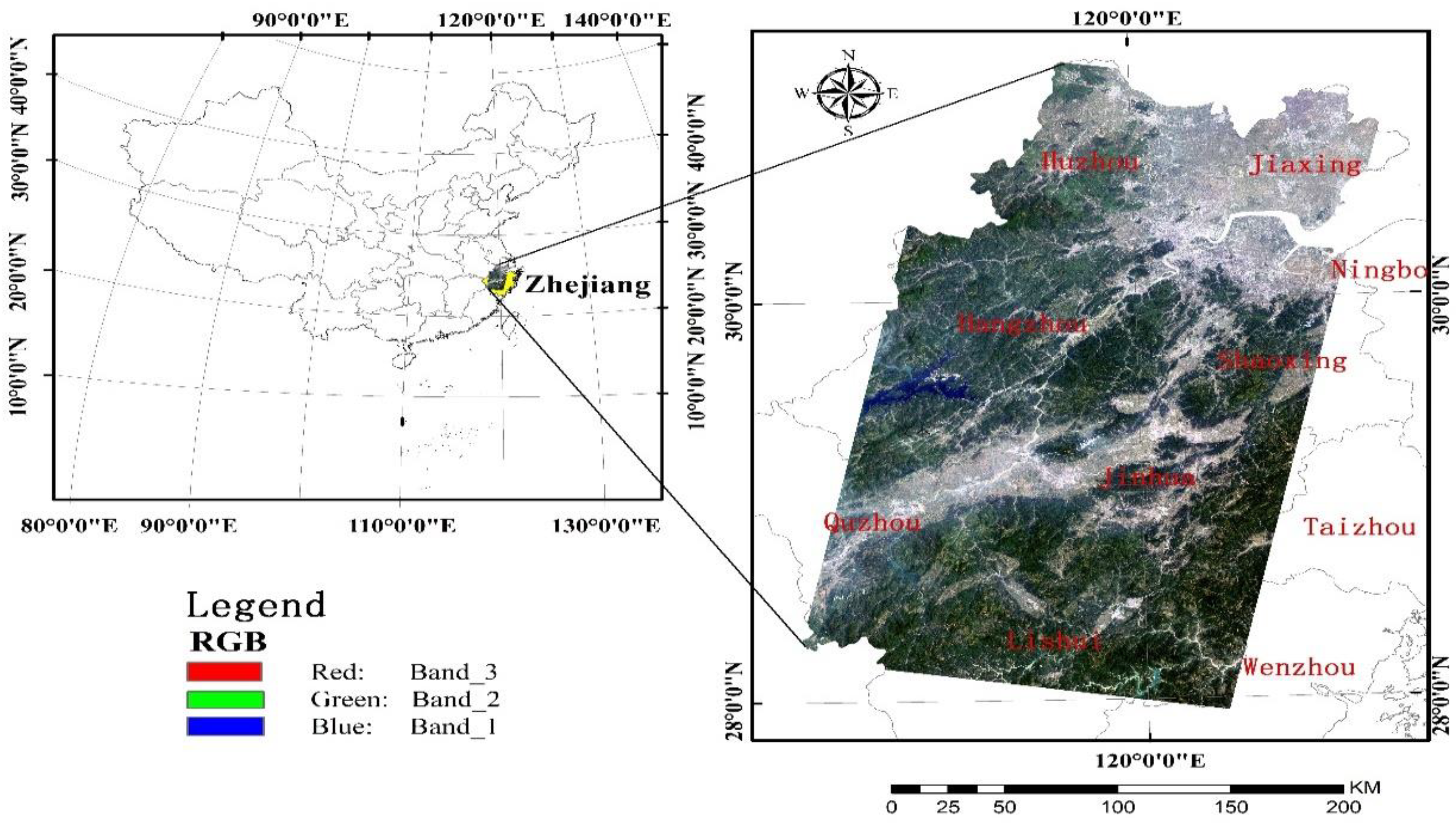
The linear regression models are often used in quantitative remote sensing, but usually there are too many variables, and the correlation between variables is high, which brings difficulties to model development and model application. Among these applications, in addition to model accuracy, the ability of the estimation method in terms of variable selection also needs to be considered. This paper takes the quantitative estimation of biomass on the aboveground biomass as an example, and comprehensively considers the conventional precision indicators, PE, ME, model parameter stability, variable selection stability and variable selection ability, and conducts comparative study on the 10 common parameter estimation/variable selection methods. Research data includes Landsat TM data, its derived texture data, and field plot biomass data measured in the sample field. As an article that specially focuses on variable selection methods, the number of variables selected by each method is an important factor that needs consideration. Since the mean of variables selected is quite different, the analysis of adjustment of the degree of freedom was made in this paper.

(1) About OLS and RR. RR completely lacks variable selection ability, and OLS is not used in variable selecting generally. They are mainly used to compare with other methods that have variable selection ability in this paper. If the six indicators involving R², RMSE, RMSEr, PE, ME and ME/PE were taken into consideration, RR had the best performance among the ten methods and OLS was listed in the third before adjustment of the degree of freedom; and after adjustment, RR was listed 4th place and OLS took the 7th place. According to the significance test of R², $\mathrm{RR}\underset{0.01}{>}(\mathrm{all}\mathrm{the}\mathrm{other})$, $\mathrm{OLS}\underset{0.05/0.01}{>}(\mathrm{AIC},\mathrm{NNG})$. RR has obvious advantages, while OLS lacks obvious advantages before we adjust the degree of freedom. After the adjustment of the degree of freedom, $\mathrm{RR}\underset{0.05/0.01}{>}\left(\mathrm{Cp},\mathrm{AIC},\mathrm{NNG},\mathrm{OLS}\right)$, $\mathrm{OLS}\underset{0.05/0.01}{=}(\mathrm{Cp},\mathrm{NNG})$. So, it can be found that after adjustment, RR’s advantages were weakened obviously, while OLS completely has no advantage, having only the same accuracy as the other two methods. In terms of parameter stability, RR takes the first place and OLS is ranked as No.7. Although RR has higher parameter stability, its precision performance is not outstanding, while OLS has no obvious advantages in any aspect. OLS is easily subject to collinearity effect, so it is not applied in the case of many variables and severe collinearity. Studies on other fields also show that OLS is inferior to the coefficient shrink method in the prediction accuracy, RMSE, etc. [21,22,26]. Although RR has anti-collinearity ability, it completely lacks variable selection ability. Main variables among lots of variables can’t be found by the RR method, meanwhile, a model can’t be simplified, so RR is also not applicable. RR is far inferior to coefficient shrink and subset selection methods in reducing of complexity of the model. These issues have been demonstrated in the previous studies [23,24,25,26].

The following discussion doesn’t cover RR and OLS, and we only consider situations that involve the adjustment of the degree of freedom.

Conclusion on a general analysis of frequently-used evaluation indicators and PE. Through the comprehensive analysis of indicators including R², RMSE, RMSEr, PE, ME, ME/PE, etc., it can be found that BIC> ADALASSO> LASSO> AIC> SCAD>SR>NNG>Cp; BIC is the best, and Cp, NNG and SR are relatively poor.

Significance test of the coefficient of determination difference. Here we see $\left(\mathrm{BIC},\mathrm{ADALASSO},\mathrm{LASSO}\right)\underset{0.05/0.01}{>}\left(\mathrm{SR},\mathrm{AIC},\mathrm{Cp},\mathrm{NNG}\right)$, the three former coefficients are significantly superior to the later four coefficients at the level of 0.01 or 0.05. There are no significant differences among the former three coefficients, and the same among the latter four coefficients. In addition, $\mathrm{SCAD}\underset{0.05/0.01}{>}(\mathrm{AIC},\mathrm{Cp},\mathrm{NNG})$, $\mathrm{SR}\underset{0.05/0.01}{>}\left(\mathrm{Cp},\mathrm{NNG}\right)$.

Stability of model coefficients. Through the analysis of the ratio of variance within parameters to that among parameters based on the same method, a conclusion can be drawn that BIC > LASSO > ADALASSO > SR > SCAD > AIC > NNG > Cp. Stability of coefficients reflects changes of parameters found when models were established based on data having differences through a method. Higher stability means small changes, and lower stability means big changes. A good method should have high parameter stability.

Variable selection stability. Through the analysis of the ratio of variance of indicative data within parameters to that of indicative data among parameters based on the same method, it can be drawn that BIC > SR > LASSO > SCAD > ADALASSO > AIC > Cp > NNG. Variable selection stability reflects changes of explanatory variables selected when models were constructed based on data having differences through a method. Higher stability indicates higher possibility that the same variables are selected when models are constructed based on data having differences. Low stability indicates big changes in variable selecting. A good method should have high variable selection stability.

Variable selection ability. Through the analysis of the number and changes of explanatory variables used to construct models by different methods, and comparison of the mean, median, maximum, minimum, range and standard deviation of number of variables, these eight methods can be ranked as BIC > SR > Cp > ADALASSO > AIC > SCAD > LASSO > NNG. The mean of number of variables is between 2.32 and 10.06; the median is between two and 10; the maximum value is between three and 21; the minimum value is between two and six; the range is from one to 19; the standard deviation is between 0.4712 and 4.9132. All indicators under the BIC method are the best, number of variables is 2–3, and the range is one. The BIC method is the optimization of AIC. In terms of penalty, when n > 8, k ln(n) > 2k, so BIC gives more penalty to model parameters than AIC when there exists a large amount of data. This leads to that BIC tends to choose a simple model with a small number of variables. NNG has the worst performance. The number of variables selected by this method is up to 21, the minimum number is only two, and the range reaches 19. Overall, the variable selection ability of the subset selection method is stronger than the coefficient shrink method.

Comprehensive evaluation of the eight methods having variable selection ability. Sequence numbers of each method in each indicator are shown in

Table 10. General evaluation.

	Subset Selection Methods				Coefficient Shrink Methods
Indicators	BIC	SR	Cp	AIC	ADALASSO	SCAD	LASSO	NNG
Frequently-used Indicators	1	6	8	4	2	5	3	7
Parameter Stability	1	4	8	6	3	5	2	7
Variable selection stability	1	2	7	6	5	4	3	8
Variable selection ability	1	2	3	5	4	6	7	8
Significance test of R2	1	3	4	4	1	2	1	4
Mean	1.0	3.4	6.0	5.0	3.0	4.4	3.2	6.8

. According to the evaluation sequence number, BIC gives the best performance, and it takes the first place in terms of all indicators. Overall, NNG, Cp and AIC perform badly. Performance of other methods evaluated through various indicators is quite different. ADALASSO is good in terms of accuracy, but it is just Ok in the aspects of variable stability and variable selection ability. LASSO is particularly poor in terms of variable selecting, but it is not bad in other aspects. SCAD has a weak overall performance. SR has stronger ability to choose variables, but it has bad performance in terms of common performance. There are no significant differences in prediction accuracy and other indicators according to the study results. From this point of view, variable selection ability is a factor that should be given much more attention, so SR, as a common method, is used frequently due to its strong ability to choose variables. Among the eight methods, only BIC and AIC are both based on the Maximum Likelihood Estimation. AIC performs not as good as BIC does and the reason maybe the different penalty function. The best BIC performance may be related to the maximum likelihood estimate and its penalty function.

In 400 (8 × 5 × 10) experiments of eight methods with variable selection ability in five ten-fold cross validations, explanatory variables B7, B7_W9_CC and B7_W5_ME are mostly used, which are the short-wave infrared band and two texture features of the short-wave infrared band. From this, it can be known that the short-wave infrared band and its special texture features play an important role in the estimation of forest biomass. In the estimation model of biomass, a short-wave infrared band is more important than a visible-light band because the former is more sensitive to humidity and shadow information in the structure of forest, and atmospheric condition has a smaller influence on it, in comparison with other bands (e.g., visible light band and near infrared band).

7. Conclusions

By comparing four methods of subset selection and four methods of compression coefficients with variable selection ability, and OLS and RR without variable selection ability, the following conclusions are obtained:

• RR has high parameter stability and anti-multicollinearity ability, but its accuracy performance is not outstanding, OLS has no obvious advantages in any aspect. Both methods lack the ability to select variables, so they are not applicable when there are many variables.
• By comparing the R², RMSE, RMSEr, PE, ME and ME/PE indicators, the order of performance is as follows: BIC> ADALASSO> LASSO> AIC> SCAD>SR>NNG>Cp.
• By comparing the differences in the significance of coefficients of determination, the result is as follows, $(\mathrm{BIC},\mathrm{ADALASSO},\mathrm{LASSO})\underset{0.05/0.01}{>}(\mathrm{SR},\mathrm{AIC},\mathrm{Cp},\mathrm{NNG})$, $\mathrm{SR}\underset{0.05/0.01}{>}(\mathrm{Cp},\mathrm{NNG})$ and $\mathrm{SCAD}\underset{0.05/0.01}{>}(\mathrm{AIC},\mathrm{Cp},\mathrm{NNG})$.
• Comparing the stability of the coefficients of models, the following result is obtained: BIC > LASSO > ADALASSO > SR > SCAD > AIC > NNG > Cp.
• Comparing the stability of variable selection, the following result is obtained, BIC > SR > LASSO > SCAD > ADALASSO > AIC > Cp > NNG.
• Comparing the capability of variable selection, the following result is obtained: BIC>SR> Cp> ADALASSO> AIC> SCAD> LASSO> NNG.
• Comprehensive evaluation of eight methods with variable selection ability. The BIC method has shown the best performance, while NNG, Cp, and AIC were generally poor. Other methods have a large difference in performance on each indicator. ADALASSO performs well in terms of accuracy, but performs not so bad in terms of variable stability and variable selection capability. LASSO is particularly poor in terms of variable selection, but relatively well in other aspects. SCAD is also weak overall; however, it is poor in common indicators. Variable selection ability is a factor that should be given much more attention, so SR, as a common method, is used frequently due to its strong ability to choose variables.
• The most frequently selected variables are B7, B7_W9_CC and B7_W5_ME, which are the short-wave infrared and two texture features of short-wave infrared, respectively. It can be seen that the short-wave infrared band and its texture features are important in forest biomass estimation.

In this paper, the model construction methods are evaluated by five categories of indicators: Commonly used indicators, prediction error and model error, model parameter stability, variable selection stability and variable selection ability. For the same method, different indicators may have different performance, which brings difficulties to the method selection. Therefore, comprehensive consideration is needed. For one method, its advantage is particularly obvious on a certain indicator, or the disadvantage is particularly obvious. Such an indicator needs to be given more attention. You can give priority to this method or give up the method. On the contrary, there is no obvious advantage or disadvantage in a certain indicator, so one does not need to pay too much attention on such an indicator, that is, such an indicator has little effect on the selection of methods. In addition, we can consider the main indicators based on the needs. For example, when the main purpose is to choose a simpler model, we can pay more attention to variable selection ability, variable selection stability and model parameter stability, etc. The other indicators are only for reference.

References

1. Achard, F.; Eva, H.D.; Mayaux, P.; Stibig, H.J.; Belward, A. Improved estimates of net carbon emissions from land cover change in the tropics for the 1990s. Glob. Biogeochem. Cycles 2004, 18. [Google Scholar] [CrossRef]
2. Frolking, S.; Palace, M.W.; Clark, D.B.; Chambers, J.Q.; Shugart, H.H.; Hurtt, G.C. Forest disturbance and recovery: A general review in the context of spaceborne remote sensing of impacts on aboveground biomass and canopy structure. J. Geophys. Res. Biogeosci. 2015, 114, G00E02. [Google Scholar] [CrossRef]
3. Hansen, M.C.; Potapov, P.V.; Moore, R.; Hancher, M.; Turubanova, S.A.; Tyukavina, A.; Thau, D.; Stehman, S.V.; Goetz, S.J.; Loveland, T.R.; et al. High-Resolution Global Maps of 21st-Century Forest Cover Change. Science 2014, 342, 850–853. [Google Scholar] [CrossRef]
4. Houghton, R.A. Aboveground Forest Biomass and the Global Carbon Balance. Glob. Chang. Biol. 2005, 11, 945–958. [Google Scholar] [CrossRef]
5. Hese, S.; Lucht, W.; Schmullius, C.; Barnsley, M.; Dubayah, R.; Knorr, D.; Neumann, K.; Riedel, T.; Schröter, K. Global biomass mapping for an improved understanding of the CO2 balance—the Earth observation mission Carbon-3D. Remote Sens. Environ. 2005, 94, 94–104. [Google Scholar] [CrossRef]
6. Lieth, H.F.H. Patterns of Primary Production in the Biosphere; Dowden, Hutchinson and Ross: New York, NY, USA, 1978. Available online: http://www.nal.usda.gov/ (accessed on 14 June 2019).
7. Sedjo, R.A. The carbon cycle and global forest ecosystem. Water Air Soil Pollut. 1993, 70, 295–307. [Google Scholar] [CrossRef]
8. Waring, R.H.; Running, S.W. Forest Ecosystems, 3rd ed.; Analysis at Multiple Scales; Elsevier Academic Press: San Diego, CA, USA, 2007. [Google Scholar]
9. Le Toan, T.; Quegan, S.; Davidson, M.W.J.; Balzter, H.; Paillou, P.; Papathanassiou, K.; Plummer, S.; Rocca, F.; Saatchi, S.; Shugart, H.; et al. The BIOMASS mission: Mapping global forest biomass to better understand the terrestrial carbon cycle. Remote Sens. Environ. 2011, 115, 2850–2860. [Google Scholar] [CrossRef] [Green Version]
10. Lu, D.; Chen, Q.; Wang, G.; Liu, L.; Li, G.; Moran, E. A survey of remote sensing-based aboveground biomass estimation methods in forest ecosystems. Int. J. Digit. Earth 2014, 9, 63–105. [Google Scholar] [CrossRef]
11. Segura, M.; Kanninen, M.J.B. Allometric models for tree volume and total aboveground biomass in a tropical humid forest in Costa Rica. J. Biol. Conserv. 2005, 37, 2–8. [Google Scholar]
12. Seidel, D.; Fleck, S.; Leuschner, C.; Hammett, T. Review of ground-based methods to measure the distribution of biomass in forest canopies. Ann. For. Sci. 2011, 68, 225–244. [Google Scholar] [CrossRef] [Green Version]
13. Wang, G.; Zhang, M.; Gertner, G.Z.; Oyana, T.; Mcroberts, R.E.; Ge, H. Uncertainties of mapping aboveground forest carbon due to plot locations using national forest inventory plot and remotely sensed data. Scand. J. For. Res. 2011, 26, 360–373. [Google Scholar] [CrossRef]
14. Roy, P.S.; Ravan, S.A. Biomass estimation using satellite remote sensing data—An investigation on possible approaches for natural forest. J. Biosci. 1996, 21, 535–561. [Google Scholar] [CrossRef]
15. Næsset, E.; Gobakken, T.; Bollandsås, O.M.; Gregoire, T.G.; Nelson, R.; Ståhl, G. Comparison of precision of biomass estimates in regional field sample surveys and airborne LiDAR-assisted surveys in Hedmark County, Norway. Remote Sens. Environ. 2013, 130, 108–120. [Google Scholar] [CrossRef] [Green Version]
16. Zheng, D.; Rademacher, J.; Chen, J.; Crow, T.; Bresee, M.; Le Moine, J.; Ryu, S.-R. Estimating aboveground biomass using Landsat 7 ETM+ data across a managed landscape in northern Wisconsin, USA. Remote Sens. Environ. 2004, 93, 402–411. [Google Scholar] [CrossRef]
17. Sun, G.; Ranson, K.J.; Guo, Z.; Zhang, Z.; Montesano, P.; Kimes, D. Forest biomass mapping from lidar and radar synergies. Remote Sens. Environ. 2011, 115, 2906–2916. [Google Scholar] [CrossRef] [Green Version]
18. Pavan, K.; Sharma, L.K.; Pandey, P.C.; Sinha, S.; Nathawat, M.S. Geospatial Strategy for Tropical Forest-Wildlife Reserve Biomass Estimation. IEEE J. Sel. Top. Appl. Earth Obs. Remote Sens. 2013, 6, 917–923. [Google Scholar]
19. Gao, Y.; Lu, D.; Li, G.; Wang, G.; Chen, Q.; Liu, L.; Li, D. Comparative Analysis of Modeling Algorithms for Forest Aboveground Biomass Estimation in a Subtropical Region. Remote Sens. 2018, 10, 627. [Google Scholar] [CrossRef]
20. Zhao, P.; Lu, D.; Wang, G.; Liu, L.; Li, D.; Zhu, J.; Yu, S. Forest aboveground biomass estimation in Zhejiang Province using the integration of Landsat TM and ALOS PALSAR data. Int. J. Appl. Earth Obs. Geoinf. 2016, 53, 1–15. [Google Scholar] [CrossRef]
21. Yuri, F.; Hiroshi, M.; Chihiro, M.; Ryo, A.J.I.O.; Science, V. Applying “Lasso” Regression to Predict Future Visual Field Progression in Glaucoma Patients. Investig. Ophthalmol. Vis. Sci. 2015, 56, 2334–2339. [Google Scholar]
22. Zhang, Y.; Minchin, R.E., Jr.; Agdas, D. Forecasting completed cost of highway construction projects using LASSO regularized regression. J. Constr. Eng. Manag. 2017, 143, 1–12. [Google Scholar] [CrossRef]
23. Roy, S.S.; Mittal, D.; Basu, A.; Abraham, A. Stock Market Forecasting Using LASSO Linear Regression Model; Afro-European Conference for Industrial Advancement; Springer: Cham, Switzerland, 2015; Volume 334, pp. 371–381. [Google Scholar] [CrossRef]
24. Maharlouei, N.; Raeisi, S.H.; Zohoori, D.; Lankarani, K.B. Factors Affecting Exclusive Breastfeeding, Using Adaptive LASSO Regression. Int. J. Community Based Nurs. Midwifery 2018, 6, 260–271. [Google Scholar]
25. Raeisi, S.H.; Pourahmad, S.; Ayatollahi, S.M. Identifying the Prognosis Factors in Death after Liver Transplantation via Adaptive LASSO in Iran. J. Environ. Public Health 2016, 2016, 7620157. [Google Scholar]
26. Zhang, Y.F.; Liu, J.H.; Li, X.X.; He, X.P.; Xu, L. Selection of Key Process Parameters for Controlling Tobacco Moisture Based on Lasso Family Models. Boletín Técnico 2017, 55, 101–110. [Google Scholar]
27. Yuan, W.; Jiang, B.; Ge, Y.; Zhu, J.; Shen, A. Study on Biomass Model of Key Ecological Forest in Zhejiang Province. J. Zhejiang For. Sci. Technol. 2009, 29, 1–5. [Google Scholar]
28. Chander, G.; Markham, B.L.; Helder, D.L. Summary of current radiometric calibration coefficients for Landsat MSS, TM, ETM+, and EO-1 ALI sensors. Remote Sens. Environ. 2009, 113, 893–903. [Google Scholar] [CrossRef]
29. Reese, H.; Olsson, H. C-correction of optical satellite data over alpine vegetation areas: A comparison of sampling strategies for determining the empirical c-parameter. Remote Sens. Environ. 2011, 115, 1387–1400. [Google Scholar] [CrossRef] [Green Version]
30. Cutler, M.E.J.; Boyd, D.S.; Foody, G.M.; Vetrivel, A. Estimating tropical forest biomass with a combination of SAR image texture and Landsat TM data: An assessment of predictions between regions. Isprs J. Photogramm. Remote Sens. 2012, 70, 66–77. [Google Scholar] [CrossRef] [Green Version]
31. Breiman, L. Better Subset Regression Using the Nonnegative Garrote. Technometrics 1995, 37, 374–384. [Google Scholar] [CrossRef]
32. Zhang, P. Model Selection Via Multifold Cross Validation. Ann. Stat. 1993, 21, 299–313. [Google Scholar] [CrossRef]
33. Molinaro, A.M.; Richard, S.; Pfeiffer, R.M. Prediction error estimation: A comparison of resampling methods. Bioinformatics 2005, 21, 3301–3307. [Google Scholar] [CrossRef]
34. Wang, D.R.; Zhang, Z.Z. Variable Selection for Linear Regression Models: A Survey. J. Appl. Stat. Manag. 2010, 29, 615–627. [Google Scholar] [CrossRef]
35. Akaike, H. Statistical predictor identification. Ann. Inst. Stat. Math. 1970, 22, 203–217. [Google Scholar] [CrossRef]
36. Schwarz, G. Estimating the dimension of a model. Ann. Stat. 1978, 6, 461–464. [Google Scholar] [CrossRef]
37. Mallows, C.L. Some Comments on CP. Technometrics 2000, 42, 87–94. [Google Scholar]
38. Breiman, L. Heuristics of Instability and Stabilization in Model Selection. Ann. Stat. 1996, 24, 2350–2383. [Google Scholar] [CrossRef]
39. Tibshirani, R. Regression Shrinkage and Selection via the Lasso. J. R. Stat. Soc. 1996, 58, 267–288. [Google Scholar] [CrossRef]
40. Hui, Z. The Adaptive Lasso and Its Oracle Properties. J. Am. Stat. Assoc. 2006, 101, 1418–1429. [Google Scholar] [Green Version]
41. Huang, J.; Ma, S.; Zhang, C.H. Adaptive LASSO for sparse high-dimensional regression. Stat. Sin. 2008, 18, 1603–1618. [Google Scholar]
42. Fan, J.; Li, R. Variable selection via nonconvave penalized likelihood and its oracle properties. J. Am. Stat. Assoc. 2001, 96, 1348–1360. [Google Scholar] [CrossRef]
Figure 1. Zhejiang province in Eastern China (left); and the study area shown in a natural color composite image from Landsat TM (right).
Remotesensing 11 01437 g001
Figure 2. Relationship between y ^ and ε .
Remotesensing 11 01437 g002
Figure 3. Normality Test.
Remotesensing 11 01437 g003
Figure 4. Test for a of smoothly clipped absolute deviation (SCAD).
Remotesensing 11 01437 g004