Mineral Classification of Soils Using Hyperspectral Longwave Infrared (LWIR) Ground-Based Data

Abstract

Soil mineralogy is an important factor affecting chemical and physical processes in the soil. Most common minerals in soils—quartz, clay minerals and carbonates—present fundamental spectral features in the longwave infrared (LWIR) region. The current study presents a procedure for determining the soil mineralogy from the surface emissivity spectrum. Ground-based hyperspectral LWIR images of 90 Israeli soil samples were acquired with the Telops Hyper-Cam sensor, and the emissivity spectrum of each sample was calculated. Mineral-related emissivity features were identified and used to create indicants and indices to determine the content of quartz, clay minerals, and carbonates in the soil in a semi-quantitative manner—from more to less abundant minerals. The resultant mineral content was in good agreement with the mineralogy derived from chemical analyses.

1. Introduction

Soil is a complex material that is extremely variable in its physical and chemical composition. It consists of weathered rocks of the Earth’s crust and is continuously evolving and changing. The upper layer is the most important part of the soil body, containing plant litter, water, roots, micro and macro fauna, and minerals that are formed in situ or transferred to the area by runoff, dust storms, or human activity. The soil surface is exposed to all remote-sensing methods. Hyperspectral remote sensing, especially in the visible–short wavelength infrared region, 0.4–2.5 µm, has been shown to be an invaluable tool for determining and mapping soil properties, using laboratory, airborne, and spaceborne sensors (e.g., [1,2,3,4,5,6]). However, recent studies have shown that the thermal infrared region, in both the mid wavelength infrared (3–5 µm) and the long wavelength infrared (LWIR, 8–12 µm) regions can provide quantitative information on soil properties, such as texture, carbon and nitrogen content, and pH, especially when large datasets are processed with statistical models (e.g., [7,8,9,10,11]). Soil mineralogy is an important factor in determining its properties, quality, and growth potential, and is extensively used as a diagnostic criterion in comprehensive soil classification. The most common minerals in soils, quartz, clay minerals, and carbonates, present with fundamental spectral features in the thermal infrared, and mainly in the LWIR region due to the fundamental vibration modes of the silicon–oxygen bond (Si–O) in quartz and clay minerals, and the carbon–oxygen bond (C–O) in carbonates. Recently, we presented a procedure that can be applied to hyperspectral LWIR images to calculate surface emissivity, an important variable for mineral mapping, and to identify the dominant minerals, quartz, feldspars, clay minerals, gypsum, and carbonates in rocks [12,13]. Nevertheless, hyperspectral remote sensing in the LWIR region, although used with significant success for the mapping of the content of minerals on rock surfaces (e.g., [14,15]), has not been fully implemented for the complex and dynamic soil material, and its potential has not yet been fully exploited.

The current study makes use of ground-based hyperspectral LWIR images, acquired with the Telops Hyper-Cam hyperspectral sensor [16], to calculate the emissivity spectra of soil samples, representing the soil’s chemical and physical properties, and then to analyze them to identify quartz, clay minerals, carbonates, and their abundance, in each sample. The resultant mineral content was correlated to the chemical elements’ abundance and the mineral composition as obtained from chemical analyses.

2. Materials and Methods

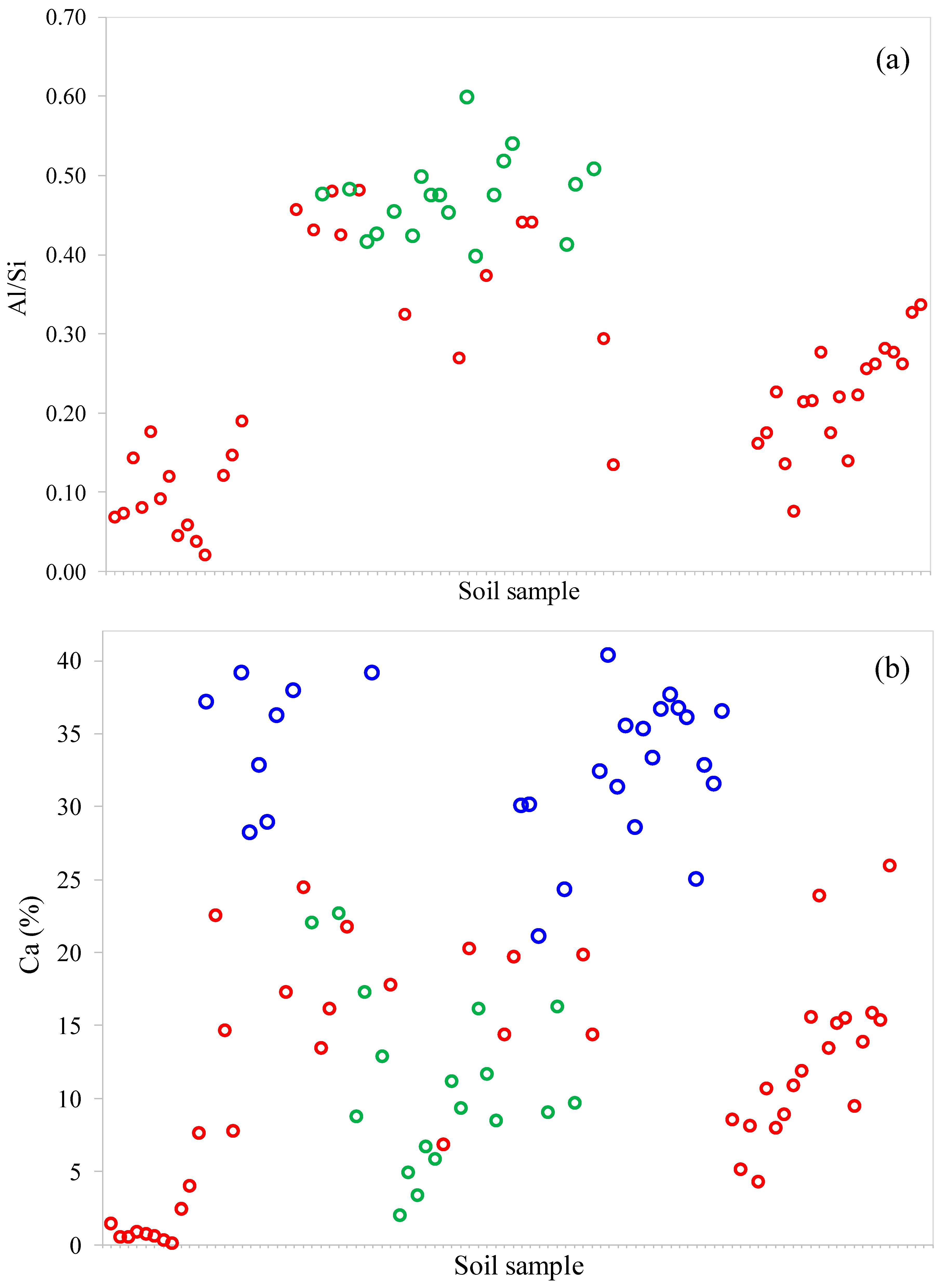
2.1. Soil Samples and Chemical Analyses

Ninety soil samples from the legacy soil spectral library of Israel, representing different formation conditions―climate, origin, and topography―were collected from the surface (0–5 cm depth) at different sites in Israel. The soils were air-dried and gently crushed to a grain size of ≤2 mm. Elemental analysis was carried out using the X-ray fluorescence (XRF) method [17]. X-ray powder diffraction (XRD) patterns of the samples were obtained using a Philips Model 1010 X-ray diffractometer with Fe-filtered CoKa radiation [18], to determine the mineralogy of each soil sample. The abundance of silicon (Si, dominant in quartz and clay minerals), aluminum (Al, dominant in clay minerals) and calcium (Ca, dominant in carbonates), and the mineral content in selected soil samples are given in

Table 1. Element abundance and mineralogy of soil samples.

Soil (Symbol, USDA Name)	Element Abundance (%)			Mineral Abundance (%)
	Si	Al	Ca	Quartz	Clay Minerals a	Carbonates b
E2, Rhodoxeralf	91.6	6.78	0.57	90	5	0
E7, Rhodoxeralf	87.2	10.5	0.30	75	15	1
C4, Haploxeroll	67.2	12.8	7.80	55	30	12
B8, Haploxeroll	42.0	17.8	17.3	30	40	31
A3, Rhodoxeralf	51.5	24.4	3.37	35	58	2
H2, Xerert	41.1	24.6	11.2	4	67	21
K2, Calciorthid	21.1	7.60	35.3	15	0	60
O3, Torriorthent	26.4	8.04	31.3	25	10	59
P3, Torriorthent	25.3	5.76	36.5	25	7	68
H11, Haplargid	29.7	4.44	30.1	36	10	54
H14, Xerert	38.4	18.7	16.3	25	45	28
S19, Torriorthent	35.4	11.9	26.0	47	10	43

^a Clay minerals refer to smectite, illite, and kaolinite. ^b Carbonates refer to calcite (mainly) and dolomite.

.

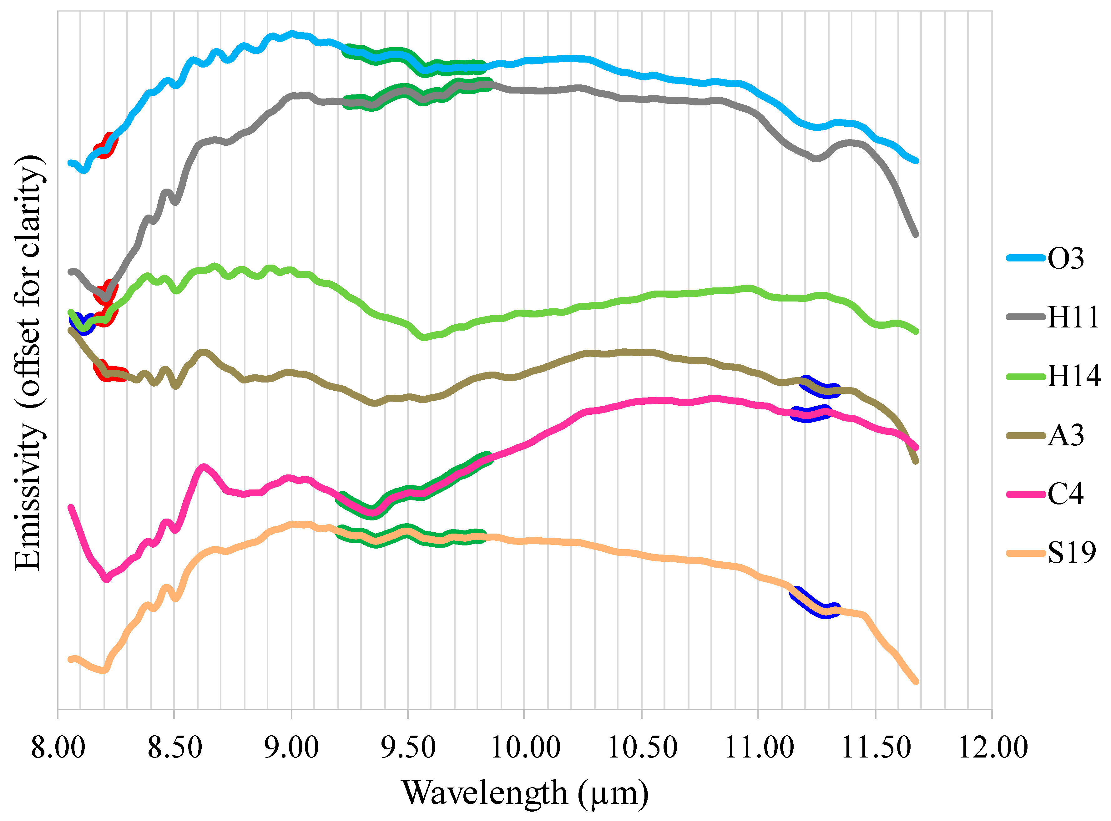
2.2. Spectral Measurements and Data Analysis

Ground-based images of the 90 soil samples were acquired with the Telops Hyper-Cam, covering the LWIR spectral region (8.0–11.7 µm) with 122 bands and a spectral resolution of 4 cm⁻¹. The samples were placed at a distance of about 2 m from the sensor, exposed to the sun (with an outdoor air temperature of ~30 °C) for about an hour, and then the LWIR images (see example in Figure 1a) were taken. The at-sensor radiance at wavelength λ (L_sλ) measured from each soil pixel in the image consisted of two components (as explained in [19]):

L_sλ = ε_λL_bλ(T) + (1 − ε_λ)L_dλ

(1)

where ε_λL_bλ(T) is the surface emission at wavelength λ with ε as the surface emissivity, and L_b(T) as the radiance from a blackbody at surface temperature T; (1-ε_λ)L_dλ is the surface reflection of the radiance incident on the surface from the atmosphere at wavelength λ with L_d as the downwelling radiance. The emissivity spectrum of each pixel was calculated according to Equation (1), with L_b(T) as the fitted tangent blackbody radiation curve, applying the specialized algorithm described in [19], and downwelling radiance (L_d) as the radiance measured from a gold plate [20] (Figure 1b). The emissivity spectrum of each soil sample was analyzed to determine its mineral content.

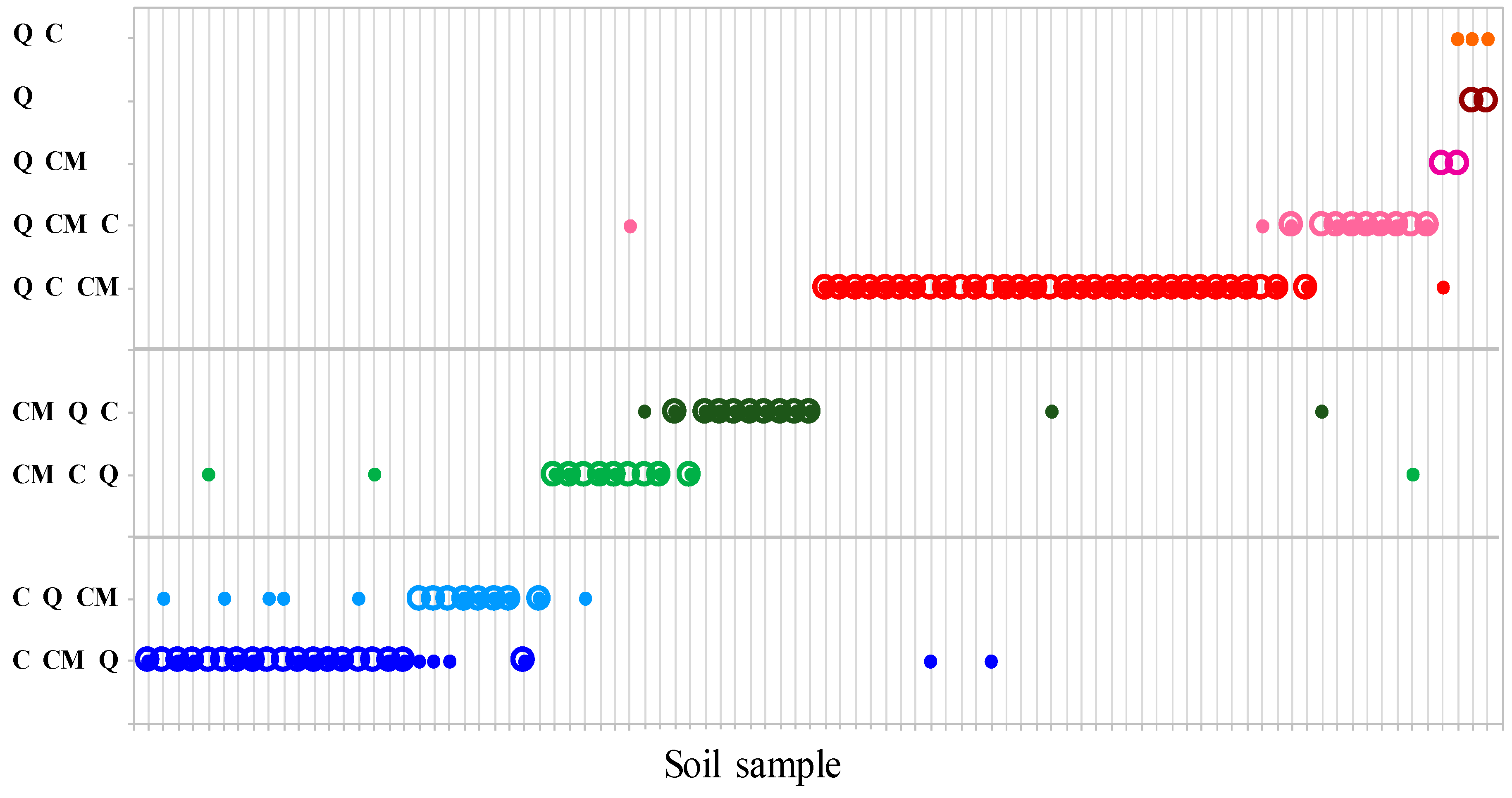
3. Results and Discussion

The content of the minerals quartz, clay minerals and carbonates in each sample was determined based on the absorption features in the emissivity spectrum, as demonstrated in Figure 2 and Figure 3. A triplet-like absorption feature with minima at 8.21 µm, 8.85 µm, and 9.33 µm (Figure 2a) indicates the presence of both quartz and clay minerals (e.g., soil E2). The ratio between the minimum values, and the wavelength of the third minimum, depend on the relative amounts of quartz and clay minerals in the soil. A decrease in the amount of quartz with an increase in the amount of clay minerals reduces the value of the absorption at 8.21 µm and shifts the absorption at 9.33 µm to 9.36–9.56 µm (e.g., soil A3). On the other hand, a minimum in the 8.06–8.12 µm range and/or a noticeable absorption feature between 10.20 µm and 11.40 µm, as demonstrated in Figure 3, indicates the presence of carbonates in the soil. The associated emissivity features of pure minerals are given in Figure 4.

The aforementioned mineral-related emissivity features were used to create spectral indicants, described in

Table 2. Spectral indicants of minerals.

Most Abundant Mineral	Spectral Indicant
Clay minerals	Nελ = 9.56µma < Nελ = 8.21µm and Nελ = 8.21µm > 0.98
Carbonates	ελ = 8.06-8.12µmb < ελ = 8.21µm and/or Nελ = 11.24µm < 0.995 with Nελ = 8.21µm > 0.98
Quartz	Excluding the above

^a Nε is the normalized emissivity value at the indicated wavelength. ^b ε is the emissivity value in the indicated wavelength range.

, to identify the most abundant mineral(s) in each soil sample. These were then used to classify the samples into three soil types: CM (clay minerals as most abundant minerals), C (carbonates as most abundant minerals), and Q (quartz as most abundant mineral).

The spectral-based classification fit the XRD analysis results in most (90%) of the soil samples (Figure 5), as well as the elemental analysis results (Figure 6). The Al/Si values of the CM-type soils were larger than most Al/Si values of the Q-type soils (Figure 6a). In general, a larger Al/Si value in the sample indicates a higher concentration of clay minerals than quartz. The abundance of Ca (indicating the concentration of carbonates) in soils classified as a C-type was larger than in soils classified as a CM or Q-type (Figure 6b).

Once the most abundant minerals were determined, we turned to identifying the less abundant minerals in each soil sample using two indices that were created based on their mineral-related emissivity features:

SQCMI (Soil Quartz Clay Mineral Index) = Nε_{λ = 9.56 µm}/(Nε_{λ = 8.21 µm} x Nε_{λ = 8.85 µm})

(2)

and

SCI (Soil Carbonate Index) = Nε_{λ = 11.24 µm} x Nε_{λ = 10.51 µm}/Nε_{λ = 8.85 µm}

(3)

where Nε is the normalized emissivity value at the indicated wavelength.

In general, a larger SQCMI value indicates a higher Si/Al ratio (Figure 7a), suggesting a lower concentration of clay minerals relative to quartz; a smaller SCI value indicates a higher concentration of carbonates in the soil sample (Figure 7b).

Comparing the index values with the chemical analysis resulted in spectral indicants, described in

Table 3. Spectral indicants of the relative amounts of minerals.

Soil Type	Indicant	Relative Amount of Mineral(s)
Q	SCI < 1.010	C > CM
	1.010 ≤ SCI < 1.020 and SQCMI > 1.020	C > CM
	SCI > 1.020 SCI > 1.050, SQCMI > 1.200	CM > C no C, no CM
CM	Absorption at 8.12 µm and/or SCI < 1.005	C > Q
C	SQCMI > 1.010 with Nελ = 8.21µm < 0.990	Q > CM

, which enabled determining the mineralogy, from more to less abundant, in each soil sample.

Emissivity spectra of selected soil samples, their indices and mineralogy are presented in Figure 8 and

Table 4. Spectral indicants and resultant mineralogy of selected soil samples.

Soil	Type	Indicants	Mineralogy (More to Less Abundant)
			Spectral-Based	XRD Analysis
E2	Q	SQCMI = 1.072, SCI = 1.041	Q CM C	Q CM
E7	Q	SQCMI = 1.033, SCI = 1.033	Q CM C	Q CM C
C4	Q	SQCMI = 1.015, SCI = 1.010	Q CM C	Q CM C
B8	CM	SCI = 1.004	CM C Q	CM C Q
A3	CM	SCI = 1.010	CM Q C	CM Q C
H2	CM	SCI = 1.008, absorption at 8.12 µm	CM C Q	CM C Q
K2	C	SQCMI = 1.004	C CM Q	C Q CM
O3	C	SQCMI = 1.000	C CM Q	C Q CM
P3	C	SQCMI = 1.020	C Q CM	C Q CM
H11	C	SQCMI = 1.017, Nελ = 8.21µm = 0.983	C Q CM	C Q CM
H14	CM	SCI = 1.002, absorption at 8.12 µm	CM C Q	CM C Q
S19	Q	SQCMI = 1.012, SCI = 0.997	Q C CM	Q C CM

, respectively.

The spectral-based full mineralogy of most (75%) soil samples fit the XRD analysis results (Figure 9).

Overall, the indicants enabled the determining of the mineral content in the soil in a semi-quantitative manner, from more to less abundant minerals.

4. Conclusions

The current study presents a procedure for determining the soil mineralogy using ground-based hyperspectral LWIR images. The emissivity spectra of 90 soil samples were calculated and analyzed to identify the most common minerals in soils, quartz, clay minerals, and carbonates, and their relative abundance in each sample. Identifying the mineral-related emissivity features and their relative intensities enabled the creation of indicants to identify the most abundant mineral(s) in each soil sample and to classify it as a Q-, CM-, or C-type soil. The spectral-based soil type classification fit the results of the XRD and elemental analyses in most (90%) of the soil samples. The relative amounts of the less abundant minerals in each soil sample were determined using two created indices―SQCMI and SCI, resulting in a semi-quantitative mineralogy determination. The spectral-based full mineralogy of most (75%) of the soil samples fit the XRD analysis results. The presence of organic matter, fertilizers, crude oil, and other contaminating materials should be studied in terms of whether and how they affect the indicant and index values, and therefore, the determination of the soil mineralogy.

The presented procedure can be used to study the effects of different processes, e.g., Aeolian processes, aquaturbation, and fire events on the soil surface mineralogy. For a known soil surface, an increase in the SQCMI value may indicate an increase in the amount of quartz, relative to clay minerals, and a decrease in the SCI value may indicate an increase in the amount of carbonates.

As hyperspectral technology in the thermal LWIR region is becoming established in the field of terrestrial mapping, it is important to study its potential for soil mapping. The ground-based procedure should be implemented for airborne hyperspectral LWIR data, and the ability to detect quartz, clay minerals, and carbonates, and to map their abundance in the soil surface and monitor mineralogical changes on a regional scale and should be studied further.

References

1. Ben-Dor, E.; Banin, A. Quantitative analysis of convolved Thematic Mapper spectra of soils in the visible near-infrared and shortwave-infrared spectral regions (0.4–2.5 μm). Int. J. Remote Sens. 1995, 16, 3509–3528. [Google Scholar] [CrossRef]
2. Chang, C.-W.; Laird, D.A.; Mausbach, M.J.; Hurburgh, C.R. Near-infrared reflectance spectroscopy–principal components regression analyses of soil properties. Soil Sci. Soc. Am. J. 2001, 65, 480–490. [Google Scholar] [CrossRef]
3. Ben-Dor, E. Quantitative remote sensing of soil properties. Adv. Agron. 2002, 75, 173–243. [Google Scholar]
4. Ben-Dor, E.; Chabrillat, S.; Demattê, J.A.M.; Taylor, G.R.; Hill, J.; Whiting, M.L.; Sommer, S. Using Imaging spectroscopy to study soil properties. Remote Sens. Environ. 2009, 113, S38–S55. [Google Scholar] [CrossRef]
5. Viscarra Rossel, R.A.; Cattle, S.R.; Ortega, A.; Fouad, Y. In situ measurements of soil colour, mineral composition and clay content by VIS–NIR spectroscopy. Geoderma 2009, 150, 253–266. [Google Scholar] [CrossRef]
6. Weng, Y.L.; Gong, P.; Zhu, Z.L. A spectral index for estimating soil salinity in the Yellow River Delta region of China using EO-1 Hyperion data. Pedosphere 2010, 20, 378–388. [Google Scholar] [CrossRef]
7. Soriano-Disla, J.M.; Janik, L.J.; Viscarra Rossel, R.A.; Macdonald, L.M.; McLaughlin, M.J. The performance of visible, near-, and mid-infrared reflectance spectroscopy for prediction of soil physical, chemical, and biological properties. Appl. Spectrosc. Rev. 2014, 49, 139–186. [Google Scholar] [CrossRef]
8. Eisele, A.; Lau, I.; Hewson, R.; Carter, D.; Wheaton, B.; Ong, C.; Cudahy, T.J.; Chabrillat, S.; Kaufmann, H. Applicability of the thermal infrared spectral region for the prediction of soil properties across semi-arid agricultural landscapes. Remote Sens. 2012, 4, 3265–3286. [Google Scholar] [CrossRef]
9. Eisele, A.; Chabrillat, S.; Hecker, C.; Hewson, R.; Lau, I.C.; Rogass, C.; Segl, K.; Cudahy, T.J.; Udelhoven, T.; Hostert, P.; et al. Advantages using the thermal infrared (TIR) to detect and quantify semi-arid soil properties. Remote Sens. Environ. 2015, 163, 296–311. [Google Scholar] [CrossRef]
10. Kopačková, V.; Ben-Dor, E.; Carmon, N.; Notesco, G. Modelling diverse soil attributes with visible to longwave infrared spectroscopy using PLSR employed by an automatic modelling engine. Remote Sens. 2017, 9, 134. [Google Scholar] [CrossRef]
11. Hutengs, C.; Ludwig, B.; Jung, A.; Eisele, A.; Vohland, M. Comparison of portable and bench-top spectrometers for mid-infrared diffuse reflectance measurements of soils. Sensors 2018, 18, 993. [Google Scholar] [CrossRef] [PubMed]
12. Notesco, G.; Ogen, Y.; Ben-Dor, E. Mineral classification of Makhtesh Ramon in Israel using hyperspectral longwave infrared (LWIR) remote-sensing data. Remote Sens. 2015, 7, 12282–12296. [Google Scholar] [CrossRef]
13. Weksler, S.; Notesco, G.; Ben-Dor, E. An automated procedure for reducing atmospheric features and emphasizing surface emissivity in hyperspectral longwave infrared (LWIR) images. Int. J. Remote Sens. 2017, 38, 4481–4493. [Google Scholar] [CrossRef]
14. McDowell, M.L.; Kruse, F.A. Integrated visible to near infrared, short wave infrared, and long wave infrared spectral analysis for surface composition mapping near Mountain Pass, California. In Algorithms and Technologies for Multispectral, Hyperspectral, and Ultraspectral Imagery XX; Proceedings of SPIE; Velez-Reyes, M., Kruse, F.A., Eds.; SPIE Press: Bellingham, DC, USA, 2015; Volume 9472. [Google Scholar] [CrossRef]
15. Hecker, C.; van Ruitenbeek, F.J.A.; Bakker, W.H.; Fagbohun, B.J.; Riley, D.; van der Werff, H.M.A.; van der Meer, F.D. Mapping the wavelength position of mineral features in hyperspectral thermal infrared data. Int. J. Appl. Earth Obs. Geoinf. 2019, 79, 133–140. [Google Scholar] [CrossRef]
16. TELOPS Hyperspectral IR Cameras. Available online: Telops.com/products/hyperspectral-cameras (accessed on 16 April 2019).
17. Ben-Dor, E.; Banin, A. Visible and near-infrared (0.4–1.1 µm) analysis of arid and semiarid soils. Remote Sens. Environ. 1994, 48, 261–274. [Google Scholar] [CrossRef]
18. Singer, A.; Berkgaut, V. Cation exchange properties of hydrothermally treated coal fly ash. Environ. Sci. Technol. 1995, 29, 1748–1753. [Google Scholar] [CrossRef] [PubMed]
19. Notesco, G.; Kopačková, V.; Rojík, P.; Schwartz, G.; Livne, I.; Ben-Dor, E. Mineral classification of land surface using multispectral LWIR and hyperspectral SWIR remote-sensing data: A case study over the Sokolov Lignite Open-Pit Mines, the Czech Republic. Remote Sens. 2014, 6, 7005–7025. [Google Scholar] [CrossRef]
20. Labsphare Infragold Targets. Available online: https://www.labsphere.com/labsphere-products-solutions (accessed on 16 April 2019).
21. The Arizona State University Spectral Library. Available online: http://speclib.asu.edu (accessed on 1 June 2019).
Figure 1. (a) Longwave infrared (LWIR) image (band 10.62 μm) of soil samples (each placed in a 17 × 22 cm box); soil C4 (pink square), and gold plate (yellow square). (b) At-sensor radiance (solid pink curve) and fitted tangent blackbody radiation (dashed pink curve) of soil C4, at-sensor radiance of gold plate (yellow curve) representing the downwelling radiance (left y-axis), calculated emissivity of soil C4 (right y-axis) with the respective ± standard deviation curves (gray). Each spectrum is the average of tens of pixels in the image.
Remotesensing 11 01429 g001
Figure 2. (a) Emissivity spectra of selected soil samples. Each spectrum is the average of tens of pixels in the calculated emissivity image. (b) Normalized emissivity spectra emphasizing indicative absorption features of quartz and clay minerals. Gray dashed lines emphasize the wavelengths mentioned in the text.
Remotesensing 11 01429 g002
Figure 3. (a) Emissivity spectra of selected soil samples; gray dashed boxes emphasize indicative absorption features of carbonates. Each spectrum is the average of tens of pixels in the calculated emissivity image. (b) Normalized emissivity spectra; gray dashed lines emphasize the wavelengths mentioned in the text.
Remotesensing 11 01429 g003
Figure 4. Emissivity spectra of pure minerals: quartz, kaolinite, kaolinite with quartz substrate (left y-axis) and calcite (right y-axis), based on [21] and resampled to the Telops Hyper-Cam spectral configuration.
Remotesensing 11 01429 g004
Figure 5. Type of each soil sample according to the most abundant mineral(s)―carbonates (blue), clay minerals (green), and quartz (red); each pair of circles (empty and filled) represent a soil sample; the spectral-based classification (empty circle) fits the XRD analysis results (filled circle) where the circle color is identical.
Remotesensing 11 01429 g005
Figure 6. The Al/Si value (a) and % Ca (b) of each soil sample; red circles represent spectral-based Q-type soils, green circles represent spectral-based CM-type soils, and blue circles represent spectral-based C-type soils.
Remotesensing 11 01429 g006
Figure 7. (a) Correlation between the % Si/% Al ratio and the calculated SQCMI value of all soil samples, excluding one brown–red sandy soil sample (brown circle). (b) Correlation between the % Ca values and the calculated SCI values of soil samples, excluding brown–red sandy soils (orange circles), characterized by relatively small amounts of carbonates.
Remotesensing 11 01429 g007
Figure 8. Emissivity spectra of selected C-type (O3, H11), CM-type (H14, A3) and Q-type (C4, S19) soil samples; bold curves represent mineral-related features of the less abundant minerals (blue for carbonates, red for quartz and green for clay minerals) in each sample.
Remotesensing 11 01429 g008
Figure 9. Mineralogy (from more to less abundant, y-axis) of each soil sample; spectral-based classification (empty circles) and XRD analysis results (filled circles).
Remotesensing 11 01429 g009