A Novel Relational-Based Transductive Transfer Learning Method for PolSAR Images via Time-Series Clustering

Abstract

The combination of transfer learning and remote sensing image processing technology can effectively improve the automation level of image information extraction from a remote sensing time series. However, in the processing of polarimetric synthetic aperture radar (PolSAR) time-series images, the existing transfer learning methods often cannot make full use of the time-series information of the images, relying too much on the labeled samples in the target domain. Furthermore, the speckle noise inherent in synthetic aperture radar (SAR) imagery aggravates the difficulty of the manual selection of labeled samples, so these methods have difficulty in meeting the processing requirements of large data volumes and high efficiency. In lieu of these problems and the spatio-temporal relational knowledge of objects in time-series images, this paper introduces the theory of time-series clustering and proposes a new three-phase time-series clustering algorithm. Due to the full use of the inherent characteristics of the PolSAR images, this algorithm can accurately transfer the labels of the source domain samples to those samples that have not changed in the whole time series without relying on the target domain labeled samples, so as to realize transductive sample label transfer for PolSAR time-series images. Experiments were carried out using three different sets of PolSAR time-series images and the proposed method was compared with two of the existing methods. The experimental results showed that the transfer precision of the proposed method reaches a high level with different data and different objects and it performs significantly better than the existing methods. With strong reliability and practicability, the proposed method can provide a new solution for the rapid information extraction of remote sensing image time series.

1. Introduction

Earth observation technology that is remote sensing-based on time-series images can obtain the dynamic change information of the Earth’s surface. Further, it has broad application prospects in the fields of resource surveying, emergency response, and surface monitoring. However, at present, the processing and analysis of time-series images, especially the collection of training samples, often requires a lot of manual intervention, and it is difficult to meet the need for the rapid processing of time-series images. Furthermore, the processed historical remote sensing data contain a lot of information and how to effectively use the historical information to assist with the processing and analysis of time-series images, and then improve the automation level of time-series remote sensing Earth observation technology, is an important problem that needs to be urgently solved.

Transfer learning technology can provide a reliable solution to the above problems. Given a source domain, a source task, a target domain, and a target task, transfer learning aims to improve the performance of the target task in the target domain using the knowledge in the source domain and source task [1].

Firstly, with regard to “what to transfer”, transfer learning can be categorized into four approaches: instance-based transfer, feature-representation-based transfer, parameter-based transfer, and relational knowledge transfer. Taking remote sensing image classification as an example, instance-based transfer methods, such as the methods proposed in [2,3,4,5,6,7,8], use partial training samples in the source domain to improve the performance of the model of the target domain in the model training. The feature-representation-based transfer methods, such as the methods proposed in [9,10,11,12], learn a more effective feature expression from the source domain, so that the target domain classifier built in the new feature space has a better performance. Parameter-based transfer methods, such as the methods proposed in [13,14,15,16], consider that the source domain classifier and target domain classifier have some of the same optimal parameters, which can be found from the source domain classifier and then used for the target domain classifier. The basic assumption behind relational knowledge transfer is that some of the relationships among the data in the source and target domains are similar, and thus knowledge of the relationships can be transferred from the source domain to the target domain. Examples of such methods include the methods proposed in [17,18,19,20].

Secondly, according to whether labeled data are available, transfer learning can be categorized into three sub-settings [1]: inductive transfer learning, when labeled data in the target domain are available; transductive transfer learning, when only labeled data in the source domain are available; and unsupervised transfer learning, when labeled data do not exist in either the source or target domain. Among the different categories of methods, there has been much research into inductive transfer learning and a number of studies of transductive transfer learning, with a few related applications. However, unsupervised transfer learning is a future research direction with only a few relevant studies conducted to date.

When applied to the information extraction of time-series images, inductive transfer learning needs to select appropriate labeled samples from the target domain. However, when the number of time-series images is large and the classes of ground objects are complex, the workload involved with selecting labeled samples from each temporal image is huge. Moreover, the inherent speckle noise of synthetic aperture radar (SAR) images further increases the difficulty of the manual selection of the labeled samples. Therefore, the dependence on the labeled target domain samples often means a reduction of the effectiveness and automation of the information extraction. Although the existing transductive transfer learning methods do not need target domain samples, they generally need to set more parameters and have weak robustness and the selection of optimal parameters often depends on expert experience. Therefore, the existing methods mentioned above have difficulty in meeting the requirements in practical applications such as emergency response, regional automatic monitoring, and so on. Considering the information contained in polarimetric synthetic aperture radar (PolSAR) time-series images, such as the spatio-temporal relational knowledge and physical scattering information, in order to use this information to avoid the dependence on labeled target domain samples, time-series clustering theory is introduced in this paper.

Time-series clustering can be defined as follows [21]: given a dataset of n time-series images $D=\left\{F_1,F_2,\cdots ,F_n\right\}$, the process of unsupervised partitioning of $D$ into $C=\left\{C_1,C_2,\cdots ,C_K\right\}$ is conducted in such a way that the homogeneous time-series images are grouped together based on a certain similarity measure. Time-series clustering is widely used in the field of data mining, in applications such as seasonal retail pattern analysis [22], seismic wave, and mining explosion analysis [23], gene expression pattern extraction [24,25], climate analysis [26], and stock market trend analysis [27]. To date, the research into time-series clustering has mainly focused on the following four aspects [1]: (1) The representation method for the time-series data [28,29,30,31,32], because an effective representation method is crucial to the subsequent clustering process. (2) The similarity or distance measure for the time-series curve, because the calculation of the distance measure needs to be balanced between computational efficiency and accuracy. Furthermore, how to match the distance measure with the representation of the time-series data is also a difficult problem. Related approaches include finding similar time points [33,34], judging the similarity of shape [32,35,36], or finding the sequence with the most similar change [37,38]. (3) Clustering algorithms, based on the representation method and the distance measure of the time-series data, use an appropriate clustering algorithm to cluster the data. Generally speaking, there are six main kinds of clustering methods: hierarchical clustering, partitioning clustering, model-based clustering, density-based clustering, grid-based clustering, and multi-step clustering. (4) The definition of cluster prototypes also has an important impact on the clustering effect [27,39,40]. There are three commonly used prototypes: a medoid as a prototype, an averaging prototype, and a local search prototype. However, most of the above studies of time-series clustering have been aimed at the application in the field of data mining, and their data representation methods, curve similarity measures, and so on, are difficult to match with the unique structural and physical significance of PolSAR data, so these methods cannot be directly applied to the field of PolSAR image processing.

In this paper, aiming at the above problems, and based on the spatio-temporal correlation of time-series samples and the characteristics of the multi-view polarization covariance matrix subject to a complex Wishart distribution, we propose a new three-phase time-series clustering algorithm, which can realize transductive label transfer from source domain to target domain, without relying on supervised target domain information. In this method, the samples from different images are first composed into time-series samples. Secondly, the time-series samples are clustered into different clusters by the time-series clustering algorithm. The time-series samples which do not change in the whole time series are then extracted from the clusters. Finally, the labels from the source domain samples are transferred to these unchanged target domain samples. For convenience of description, the proposed method is referred to as time-series clustering for transductive label transfer (TCTLT).

The rest of this paper is organized as follows. In Section 2, how to construct the TCTLT method based on the characteristics of PolSAR time-series images is introduced in detail. Then, in Section 3, the methods of accuracy evaluation are introduced, and the experimental results obtained with different time-series images are analyzed. In Section 4, the performances of TCTLT and the existing methods are discussed. Finally, our conclusions are drawn in Section 5.

2. Materials and Methods

2.1. The Introduction of Time-Series Clustering Theory into the Field of PolSAR Images

For the sample label transfer task of PolSAR time-series images considered in this paper, some important concepts are defined as follows:

(1)

Source domain: an image with plenty of labeled samples.

(2)

Source domain samples: labeled samples in the source domain image.

(3)

Target domain: other images in the time-series images, except for the source domain image.

(4)

Target domain samples: samples in the target domain images with the sample geographical location as the source domain samples, but without an object label.

(5)

Time-series samples: sample sequences consisting of samples from the same geographic location of all the sequential images, including source domain samples and target domain samples.

(6)

Time-series samples of a certain class of objects: taking the water time-series sample as an example, it is defined as a time-series sample, for which the label in the source domain image is “water”.

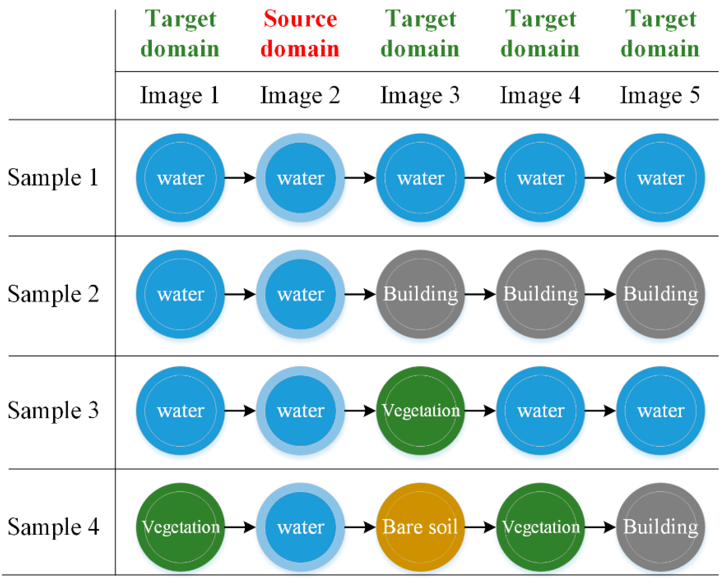
The aim of this paper is to assign class labels to the target domain samples. Although the geographic locations of target domain samples and source domain samples are exactly the same, their corresponding types of ground objects may change with time. Therefore, the class labels of source domain samples cannot be directly assigned to target domain samples, as shown in Figure 1.:

In order to avoid any confusion, “type” and “class” in this paper have different specific meanings: “type” describes the temporal variation of the time-series samples and “class” represents the label of the time-series samples in the source domain. For example, there are four types of water time-series samples in Figure 1. Their labels in the source images are all water, and the labels in the target images are not identical. Among them, the class of the object of Sample 1 does not change in the whole time series, while the class of the objects of Samples 2–4 do change in some images. Therefore, only for those time-series samples such as Sample 1 can the class labels of the source domain samples be directly assigned to the target domain samples.

In order to extract time-series samples such as Sample 1, for which the class does not change in the whole time series, we assume that each time-series sample has a value $V_i$ reflecting the corresponding object class in each image, and then a time-series sample $S=\left\{S_1,S_2,\cdots ,S_n\right\}$ can form a time-series curve $V=\left\{V_1,V_2,\cdots ,V_n\right\}$. We assume that the similarity between the same types of time-series curves is greater than that between different types of time-series curves, as shown in the following formula:

$$Similarity\left(V^i,V^i\right)>Similarity\left(V^i,V^j\right),i\ne j$$

(1)

where $V^i$ and $V^j$ are the time-series curves of time-series samples of type i and j, respectively.

Based on the similarity, the same types of time-series samples can be clustered into one group by clustering, and we can then extract the required time-series samples from the clusters. Therefore, we introduce the theory of time-series clustering, which, according to the shape, characteristics, or model of the time-series curve, clusters the curves with high similarity into one group under certain criteria.

2.2. A Three-Phase Time-Series Clustering Algorithm for PolSAR Images

To introduce the theory of time-series clustering into the clustering of PolSAR time-series samples, the following key problems need to be solved: (1) How to represent a time-series curve (that is, how to define the value of $V$). The current time-series clustering algorithms mostly use a real value to represent $V_i$, and then $V$ will be a two-dimensional curve. However, if the complex data of PolSAR images containing four polarization channels are compressed into a real value, much of the polarization information will be lost. Therefore, it is difficult for such two-dimensional curves to describe the characteristics of PolSAR time-series samples effectively, so the best way is to retain all the polarization information. (2) How to measure the similarity between the two time-series curves (that is, how to define the $Similarity$ in Equation (1)). If all of the polarization information is used to describe the time-series curve, for example, then the data points on each phase will be represented by a polarimetric covariance matrix (the dimension is $3\times 3)$. The time-series curve will then be a curve in complex space and the existing distance measures cannot be applied to such a complex curve.

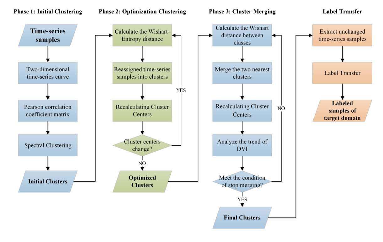
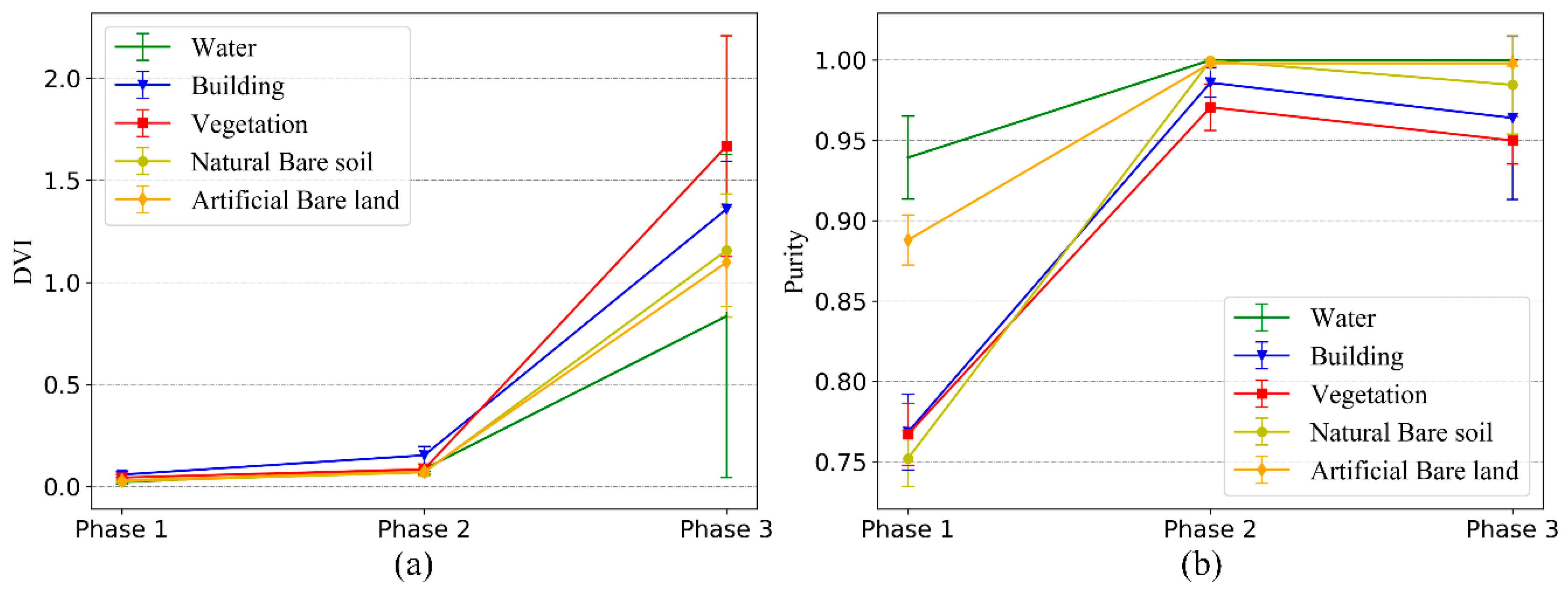
To solve the above problems, a three-phase time-series clustering algorithm is proposed in this paper. Firstly, initial clustering is carried out according to the polarimetric decomposition characteristics to provide the initial cluster centers for the next step. Secondly, optimization clustering is carried out based on the polarimetric covariance matrix and the initial cluster centers to obtain high-precision clustering results. Finally, the previous clustering results are merged so that the same types of time-series samples are further merged. The main flow chart of the algorithm is shown in Figure 2 and each phase is described in detail below.

2.2.1. Initial Clustering

The purpose of the initial clustering is to quickly obtain a set of cluster centers that are as reliable as possible as the initial value of the next phase of optimization clustering. Firstly, to achieve this goal, a two-dimensional curve is adopted for the representation of the time-series curve, i.e., for each time-series sample, the abscissa is the time series and the ordinate is a real value of the sample in that time. The real values can be expressed in the form of amplitude, intensity, or polarimetric decomposition components. However, no matter which form is adopted, a lot of polarization information will be lost, so the precision of the clustering in this phase may not be very high. Thus, in this paper, the mean value of the commonly used Pauli decomposition is used as the real value. Secondly, the common distance measures, such as dynamic time warping (DTW), the Euclidean distance, hidden Markov models, the Kullback-Leibler (KL) distance, and the Pearson correlation coefficient, can measure the similarity of two-dimensional time-series curves. The shape-based similarity measures are very effective [41], so the Pearson correlation coefficient is used as the similarity measure in this phase. For vector $X$ and vector $Y$, the formula for their Pearson correlation coefficient is as follows:

$${\rho }_{X,Y}=\frac{cov\left(X,Y\right)}{{\delta }_X{\delta }_Y}$$

(2)

where ${\rho }_{X,Y}$ is the correlation coefficient; $cov\left(X,Y\right)$ is the covariance; and ${\delta }_X$ and ${\delta }_Y$ are the standard deviation of $X$ and $Y$, respectively.

Finally, among the existing clustering methods, the two most commonly used types of methods are the hierarchical clustering methods and the partitioning clustering methods. Hierarchical clustering methods do not need the initial cluster centers, but the amount of computation is high. Partitioning clustering methods, such as the k-means algorithm, have a fast computation speed, but they require a set of initial cluster centers, and the quality of the initial cluster centers often has a significant impact on the final clustering results. In this phase, because the priority of each sample is the same, in order to obtain reliable global clustering results, the spectral clustering algorithm is used. Spectral clustering connects every two points with one edge, with each edge given a weight that represents the correlation of the two endpoints, and thus a full connection graph is constructed. The graph cut strategy is used to cut the full connection graph into many sub-graphs (clusters), with the purpose of making the weight of the edges between different sub-graphs as low as possible, and the weight of the edges in the sub-graph as high as possible [42]. This approach has the advantages of clustering in a sample space of any shape and converging to the global optimal solution, which helps to obtain a clustering result that is as reliable as possible.

The specific process of the initial clustering is shown in Phase 1 of Figure 2. Firstly, two-dimensional time-series curves of each time-series sample are constructed, where each time-series curve corresponds to a point in the full connection graph. The Pearson correlation coefficients between the two time-series curves are then calculated as the weights of their edges. Finally, similar curves are clustered globally by spectral clustering.

2.2.2. Optimization Clustering

The purpose of optimization clustering is to make full use of the information of the ground objects contained in the polarimetric covariance matrix, to optimize the initial clustering results, and thus obtain high-precision time-series clustering results.

Firstly, to preserve all the information related to the class of the objects, the whole polarimetric covariance matrix is used to represent a pixel in this phase. Thus, for a time-series sample $S_A$ and a time-series cluster center ${\omega }_m$, there are:

$$\{\begin{array}{c}{S}_A=\left\{C_{\mathrm{A}}^1,C_{\mathrm{A}}^2,\cdots ,C_A^n\right\}\\ {\omega }_m=\left\{C_m^1,C_m^2,\cdots ,C_m^n\right\}\end{array}$$

(3)

where n is the number of time-series images.

Secondly, the time-series curve represented by the above method is a curve in complex space and the conventional distance measures cannot measure the similarity between such curves. Therefore, it is necessary to design a corresponding similarity measure according to the characteristics of PolSAR time-series data.

Considering the characteristics of PolSAR data, a revised Wishart (R-Wishart) distance [43] is used to measure the distance between sample $C_A^{\mathrm{t}}$ and cluster center $C_m^{\mathrm{t}}$ at time t. It describes the similarity between the two classes of objects corresponding to the two C3 matrices. The formulas are as follows:

$$d\left(C_A^{\mathrm{t}},C_m^{\mathrm{t}}\right)=\ln \frac{\left|C_m^{\mathrm{t}}\right|}{\left|C_A^{\mathrm{t}}\right|}+Tr\left(C_m^{\mathrm{t}-1}{C}_A^{\mathrm{t}}\right)-p$$

(4)

where p is the dimension of the polarimetric covariance matrix. The smaller $d\left(C_A^{\mathrm{t}},C_m^{\mathrm{t}}\right)$ is, the more similar the object classes of $C_A^{\mathrm{t}}$ and $C_m^{\mathrm{t}}$ are.

The time-series sample $S_A$ and the time-series cluster center ${\omega }_m$ can then form an R-Wishart distance sequence $d\left(S_A,{\omega }_m\right)$ in the whole time series:

$$d\left(S_A,{\omega }_m\right)=\left\{d\left(C_A^1,C_m^1\right),d\left(C_A^2,C_m^2\right),\cdots ,d\left(C_A^n,C_m^n\right)\right\}$$

(5)

Thirdly, based on the above information, three characteristics of PolSAR time-series images are given (taking the time-series samples $S_i$, $S_j$ and the time-series cluster center ${\omega }_m$ of the same object class as examples) as follows:

(1)

The R-Wishart distance between similar objects in the same image is smaller than that between different objects.

(2)

Due to the influence of different imaging conditions, the R-Wishart distances between the same class of objects in different temporal images are different. For example, for the time-series samples $S_i$ and $S_j$, their R-Wishart distances to the cluster center ${\omega }_m$ in the first and second temporal images are as follows:

$$\begin{array}{c}d \left(C_i^1,C_m^1\right)\ne d \left(C_i^2,C_m^2\right)\\ d \left(C_j^1,C_m^1\right)\ne d \left(C_j^2,C_m^2\right)\end{array}$$

(6)

where $d\left(C_i^1,C_m^1\right)$ and $d\left(C_i^2,C_m^2\right)$ are the distance between $S_i$ and ${\omega }_m$ in the first and the second images, respectively.

(3)

Since the influence of imaging conditions on the same class of objects is similar in a single image, the change degree of the R-Wishart distance between the same class of objects in different images will be close, as shown below:

$$\left[ d\left(C_i^1,C_m^1\right)-d\left(C_i^2,C_m^2\right) \right]\cong \left[ d\left(C_j^1,C_m^1\right)-d\left(C_j^2,C_m^2\right) \right]$$

(7)

Among the three characteristics, the first characteristic shows that the distance of the same type of time-series curve is close, and the second and the third characteristics show that the shape of the same type of time-series curve is similar. Therefore, it is necessary to establish a similarity measure based on $d\left(S_A,{\omega }_m\right)$ and the above three characteristics to evaluate the shape similarity and distance of time-series curves.

First of all, we need to evaluate the shape similarity. According to the second and the third characteristics, when all the values in the distance sequence $d\left(S_A,{\omega }_m\right)$ are equal (as shown in Equation (7)), the shapes of the time-series curves of $S_A$ and ${\omega }_m$ will be exactly the same. When the value difference in $d\left(S_A,{\omega }_m\right)$ is great, their shapes will be dissimilar.

$$d\left(C_i^1,C_m^1\right)=d\left(C_i^2,C_m^2\right)=\cdots = d\left(C_i^n,C_m^{\mathrm{n}}\right)$$

(8)

Therefore, Shannon information entropy is introduced to evaluate the similarity of the time-series curves. Its formula is as follows:

$$H\left(X\right)=-{\displaystyle \sum }_{i=1}^{n}P\left(X_i\right)\log P\left(X_i\right)$$

(9)

Shannon information entropy can measure the information quantity of a random event. When $P\left(X_1\right)=P\left(X_2\right)=\cdots =P\left(X_n\right)$, the random event contains the most abundant information. By substituting $d\left(S_A,{\omega }_m\right)$ into the above formula, we can obtain the following formula:

$$H\left(d\right)=-{\displaystyle \sum }_{i=1}^{n}P\left(i\right)\log P\left(i\right),\mathrm{where}p\left(i\right)=\frac{d \left(C_A^i, C_m^i\right)}{\sum d\left(S_A,{\omega }_m\right)}$$

(10)

Equation (9) can then be used to measure the shape similarity of the two time-series curves. If $H\left(d\right)$ is larger, the shape similarity is higher.

However, according to the first characteristic, the distance of the same type of curve should be close, but Equation (9) can only measure the similarity of the shapes: when the values of each point in $d\left(S_A,{\omega }_m\right)$ are large and equal, the shapes of $S_A$ and ${\omega }_m$ will be exactly the same, but their distances will be very large, indicating that the corresponding object classes of each point are very different, which means that the time-series curves of $S_A$ and ${\omega }_m$ are not of the same type.

In order to simultaneously measure the shape and distance of the time-series curves, a penalty factor m is added to Equation (9) to restrict the absolute distance, and the following formula is obtained:

$$H_m=-{{\displaystyle \sum }}_{i=1}^{n}P\left(i\right)\log P\left(i\right)m_i,\mathrm{where}p\left(i\right)=\frac{d_i}{\sum d_i}, m_i=\frac{1}{\ln \left(1+d_i\right)}$$

(11)

The above similarity measure $H_m$ is referred to as the Wishart-entropy formula. It can measure the shape similarity and absolute distance between a time-series sample and a time-series cluster center simultaneously. The larger the value of $H_m$, the more similar the shape and distance between the time-series sample and the time-series cluster center, indicating that the time-series samples are more likely to belong to the time-series cluster center.

As shown in Phase 2 of Figure 2, the concrete steps of optimization clustering are as follows. Firstly, the similarity between each time-series sample and each time-series cluster center is calculated. The sample is then assigned to the most similar cluster center. The time-series cluster center is then recalculated after all the samples are reassigned. The above procedure is repeated until the time-series cluster centers no longer change.

2.2.3. Cluster Merging

The optimization clustering results have a high precision, but the number of clusters is still significantly larger than the number of types of time-series samples; that is, not all the time-series samples of the same type are merged into the same cluster. The first reason for this is that the number of types of time-series samples is unknown, so a large number of cluster centers is set up in the initial clustering. The second reason is the influence of the SAR imaging mode and the distribution of the ground objects, in that there will also be some differences between the same class of objects. For example, water samples may come from a calm water surface or a rough water surface and building samples may come from buildings with different dominant scattering mechanisms, leading to these time-series samples of the same type with certain differences being assigned into different cluster centers. Therefore, it is necessary to merge the time-series clusters of the same type into the same cluster, so that all the time-series samples of the same type are in the same cluster.

Cluster merging is aimed at the merging of two time-series cluster centers and it is effective enough to use a symmetric Wishart distance between classes [44] as the measure of merging. The difficulty lies in the setting of the rule for the stopping of the merging. For example, when there are four types of water time-series samples, as shown in Figure 1., the ideal result is to output four time-series cluster centers, each of which corresponds to one type of time-series sample. However, in reality, the number of types of time-series samples is unknown. If the number of cluster centers is too small, it will lead to the merging of different types of time-series cluster centers. If the number of cluster centers is too large, it may lead to the total number of unchanged samples in the final output cluster being too small. In addition, the total number of types of time-series samples in different data and different ground objects is unique, so it is impossible to obtain reliable results by setting an empirical number of clusters.

At the same time, it should be noted that the strategy of setting the number of clusters to two (i.e., dividing them into unchanged clusters and changed clusters) is not feasible, because the similarity between the changed time-series samples and the unchanged time-series samples (e.g., Sample 1 and Sample 3 in Figure 1) may be greater than that between the different types of changed time-series samples (e.g., Sample 3 and Sample 4 in Figure 1). Thus, when the number of clusters set is less than the real number of types of time-series samples, it will lead to merging between the cluster composed of changed samples and the cluster composed of unchanged samples.

In view of the above problems, we use the Dunn validity index (DVI) to assist in the automatic setting of the rule for the stopping of the merging. The DVI is defined as the shortest distance of any two clusters divided by the largest distance in any cluster. Its formula is as follows:

$$\mathrm{DVI}=\frac{\underset{i\ne j}{\min }D\left({\omega }_i,{\omega }_j\right)}{\underset{\forall k,m}{\max }d\left(S_k,{\omega }_m\right)}$$

(12)

where $D\left({\omega }_i,{\omega }_j\right)$ is the Wishart distance between two time-series clusters and $d\left(S_k,{\omega }_m\right)$ is the distance (reciprocal of $H_m$) between the time-series sample and the cluster center in a time-series cluster.

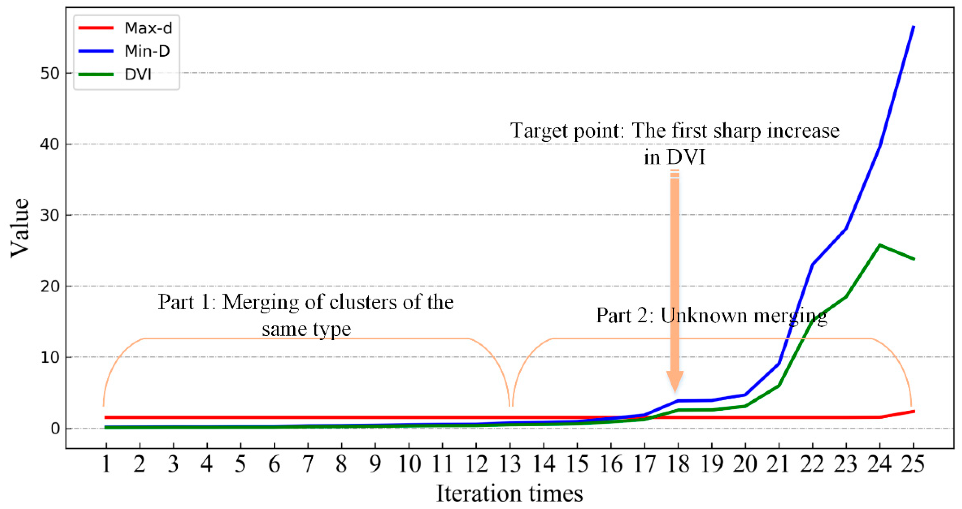
Since $\underset{\forall k,m}{\max }d\left(S_k,{\omega }_m\right)$ is the maximum distance between the sample and the cluster center in any cluster, it depends on the internal situation of a cluster. Therefore, only when incorrect cluster merges occur will the value change significantly, so it can be considered that it is almost unchanged in the process of cluster merging. However, the cluster merging involves merging the two nearest clusters at a time, so $\underset{i\ne j}{\min }D\left({\omega }_i,{\omega }_j\right)$ will increase progressively, and the DVI will also increase progressively. After each time of cluster merging, if there are two or more clusters of the same type, the change range of $\underset{i\ne j}{\min }D\left({\omega }_i,{\omega }_j\right)$ will be very small, because the distance between the same type cluster is far less than the distance between different types of clusters. If the number of the same type of cluster is less than two after a merging, the value of $\underset{i\ne j}{\min }D\left({\omega }_i,{\omega }_j\right)$ will become the distance between the two different types of clusters, which will then increase dramatically, resulting in a sharp increase in DVI value.

Therefore, the first sharp increase in DVI means that all the same types of time-series clusters are merged. Since the size of the change is a relative value, a simple but effective strategy to automatically determine when the DVI has a sharp change is described in detail below in Figure 3:

Figure 3 is the curve of DVI change with merging times when the number of clusters is merged to two. The DVI of the 18^th merging in the graph increases obviously, which indicates that all the same types of clusters have been merged at this time, so the 18^th merging is the best merging termination position.

In order to automatically locate the above position, the number of initial cluster centers is $N_1$ and the totality of the types of time-series samples is $N_2$, where $N_1$ is set artificially, and the specific value of $N_2$ is unknown, but it is related to the condition of the change of samples in each phase image, so it is generally small. If $N_1$ is set to a large value so that $N_1$ > $N_2$ * 2, then the former $N_1$/2 times of cluster merging will be the merging of the same type of cluster, and then their DVI changes can be used as a benchmark to judge the degree of DVI change in the subsequent merging.

In Figure 3, Part 1 is the reference area, Part 2 is the search area, and a threshold is set based on the change of DVI value of Part 1 (the difference between the maximum and minimum values is used as the threshold in this paper). When the change of DVI in Part 2 is greater than the threshold, the merging will stop. Based on the above strategy, the merging can be stopped automatically and effectively, without knowing the optimal number of cluster centers.

The specific process of cluster merging is shown in Phase 3 of Figure 2. Firstly, the distances between all the cluster centers are calculated using the Wishart distance between classes. The two nearest cluster centers are then merged and the cluster centers are recalculated. After each merge, the changes of the DVI curves are recorded and the above process is repeated iteratively. When the DVI increases significantly relative to the reference area after a merging, the merging does not continue and the clustering results are finally output.

2.3. Transductive Label Transfer-Based on Time-Series Clustering

The proposed three-phase time-series clustering algorithm can cluster the time-series samples into different clusters. In order to transfer the label of the source domain samples, we first need to extract the cluster we are interested in from the clustering results. In this paper, we are interested in the cluster which is composed of time-series samples that have not changed in the whole time series. Taking Figure 1 as an example, the number of samples in each type of time series (i.e., the number of samples in their corresponding time-series clusters) is $\left\{N_1,N_2,N_3,N_4\right\}$, respectively. The first type is the time-series samples that have not changed in the whole time series. In order to extract this cluster, a condition is set as follows:

$$N_1>\max \left(N_2,N_3,N_4\right)$$

(13)

The above condition can be summarized as “the number of unchanged time-series samples is dominant”. Actually, this condition is easy to meet. Firstly, for a large area in a remote sensing image, its change in the time-series images will always be gradual. Secondly, even if the ground objects change significantly, the degree of change in each image will be different. In addition, we use a uniform sampling strategy when selecting samples from the images. Thus, the number of unchanged time-series samples is often dominant, which was proved by the experiments with different data and different types of objects. Based on the above condition, the time-series cluster with the largest number of time-series samples is the one we are interested in.

After extracting the time-series samples from the clusters of interest, because the class of the objects of these time-series samples does not change in the whole time series, their class labels in the source domain images can be directly assigned to the target domain images. Thus, we can obtain a group of target domain labeled samples, i.e., the label transfers, without relying on the supervised information of the target domain images.

In this paper, the three-phase time-series clustering algorithm is applied to the transfer of sample labels. In this process, there is no need to use labeled samples in the target domain, so it is a transductive transfer method. In the process of time-series clustering, the similarity measure is constructed based on the relational knowledge between objects in the sequential images, so it is also a relational knowledge transfer method.

3. Experiments

3.1. Evaluation Methods and Experimental Setting

3.1.1. Evaluation Methods

This paper proposes a three-phase time-series clustering algorithm for transductive label transfer. Therefore, the evaluation of this method should include two aspects. The first is to evaluate the effectiveness of the proposed three-phase time-series clustering algorithm from the perspective of the time-series clustering algorithm; the second is to evaluate the label transfer precision and robustness of this method from the perspective of transfer learning.

• Evaluation of the three-phase time-series clustering algorithm

Firstly, for the evaluation of the proposed three-phase time-series clustering algorithm, it is difficult to use a unified standard to evaluate the different time-series clustering algorithms, because of the different fields, purposes and definitions of clusters. Therefore, clustering evaluation indicators are needed. According to whether there are true labels as references, the commonly used clustering evaluation indicators can be divided into internal indices and external indices [21]. External indices such as purity, the Rand index, the F-measure, and entropy evaluate the algorithm by comparing the difference between the clustering results and the true labels. Internal indices evaluate the clustering results using only the information inside the data, such as the sum of square of the errors, the DVI, the root-mean-square standard deviation, and the R-squared index. For specific tasks, the specific definitions of the above indices are not the same. In this paper, the external index of purity and the internal index of DVI are selected as the clustering evaluation indicators.

The purity of a certain class of ground objects is defined as the proportion of the samples correctly clustered to the total samples. The formula is as follows:

$$\mathrm{Purity}=\frac{N_c}{N_A}$$

(14)

where $N_C$ is the number of samples clustered correctly, $N_A$ is the total number of samples, so there are:$0<\mathrm{purity}\le 1.0$. The higher the purity, the fewer different types of time-series samples are merged into the same cluster; that is, the higher the clustering precision.

The definition of the DVI is the same as that in Section 2.2. It equals the shortest distance of any two clusters divided by the largest distance in any cluster. Because there are no real labels as reference, the DVI cannot evaluate the correctness of the clustering, and it can only measure the aggregation degree of the clustering. In this paper, with the process of merging, a larger DVI indicates that more clusters of the same type are merged together, and a smaller DVI indicates that more time-series samples of the same type are assigned into different clusters.

Therefore, the ideal clustering result is that the purity is high enough and the DVI is as large as possible. In the experiments, we compared the purity and DVI of each phase in the three-phase time-series clustering to illustrate the validity and necessity of the clustering process.

• Evaluation of label transfer precision

Because the method described in this paper is to transfer the sample labels of each class of object separately, the label transfer precision of a certain class is defined as the proportion of the samples correctly labeled to the total samples labeled as this class. The formula is as follows:

$$\mathrm{Precision}=\frac{S_c}{S_A}$$

(15)

where $S_c$ represents the samples correctly labeled, and $S_A$ represents all the samples labeled as this class.

In order to evaluate the effectiveness of the proposed method, two other transfer learning algorithms were introduced to carry out comparative experiments: transfer bagging (TrBagg) [2] and bagging-based ensemble transfer learning (BETL) [8].

TrBagg believes that the source domain data are composed of data that can represent the characteristics in the target domain and data that are not related to the characteristics in the target domain, so there is a complementary relationship between the data from the two domains. It is mainly composed of learning and filtering stages. In the learning stage, training subsets are generated by sampling from all the data and target domain labeled samples are added to train together to generate weak classifier sets. In the filtering stage, classifiers that are not helpful to the target domain tasks are filtered out from the weak classifier sets by their effectiveness in classifying the target domain labeled samples.

BETL combines source domain and target domain data to train classifiers to form a set of judgments to label the unlabeled samples in the target domain. It consists of two stages: initialization and updating. In the initialization stage, the source domain labeled sample subsets are generated and the fusion subsets are obtained by adding together all the target domain samples, and then several classifiers are trained using these subsets. In the updating stage, the unlabeled samples in the target domain are predicted using the classifiers in the previous stage and the samples with consistent prediction results are added into the target domain sample set, and then a new weak classifier is trained. In the following process, the unlabeled samples are labeled in the target domain using all the weak classifiers and the above process is repeated until a new set of weak classifiers is obtained. Finally, the above weak classifier set trained by the target domain samples is used to predict the unlabeled samples to obtain the class labels.

During a single label transfer process, the target domain of TrBagg and BETL is only one image. In the label transfer of PolSAR time-series images, when the number of images is n, the number of images in the target domain equals (n − 1), so the two methods need to transfer n − 1 times. Their input data for each time of label transfer are: a large number of labeled samples in the source domain, a small number of labeled samples in the target domain, a large number of unlabeled samples in the target domain, and a weak classifier model. The output is: a large number of labeled samples in the target domain. However, for the method proposed in this paper, all the images form the target domain, which means only one time of label transfer is needed.

Therefore, when evaluating the precision of the label transfer, TrBagg and BETL output a precision value for each class of object in each image and the method proposed in this paper only outputs a precision value for each class of object in the whole time series. Although the numbers of precision values output by the two methods are different, their meanings are the same, so they are still of comparative significance.

3.1.2. Experimental Setting

Three different groups of time-series PolSAR images were used in the experiments. The first group of images was made up of four Gaofen-3 (GF-3) images, including ascending and descending orbit images, and the use of this group of images was aimed at evaluating the transfer precision of the algorithm in time-series images with different imaging angles. The second group was made up of four RADARSAT-2 and GF-3 images, so the use of these data was aimed at measuring the applicability of the algorithm for different satellite images. The third group was made up of five RADARSAT-2 images, which was aimed at evaluating the reliability of the algorithm in time-series images with long time intervals and complex classes of objects. In order to evaluate the accuracy of each method more objectively, each method was tested 10 times on each set of data, and in each experiment, a set of experimental samples were generated randomly from the ground truth to simulate the sample selection process in a real application. The sample usage in each experiment is shown in

Table 1. Sample usage in each experiment. TCTLT: transductive label transfer; TrBagg: transfer bagging; BETL: bagging-based ensemble transfer learning.

Algorithm	Source Domain Labeled Samples	Target Domain Labeled Samples	Target Domain Unlabeled Samples
TCTLT	300/class	0/class	300/class
TrBagg	300/class	5/class	300/class
BETL	300/class	5/class	300/class

below:

Although TrBagg and BETL only need at least one labeled sample in the target domain, the stability of these two methods is poor when the target domain labeled samples are too few, so we expanded them to five in this experiment. For the selection of the weak classifier, although both TrBagg and BETL use a naive Bayes (NB) classifier as the weak classifier in the corresponding references [2,8], in order to achieve a higher precision for these two methods, after comparing various weak classifiers, we used a support vector machine (SVM) classifier as the weak classifier for TrBagg and BETL.

The experiments were conducted in 64-bit Windows 10. The programing software we used was PyCharm, and the programing language was Python. TrBagg and BETL were also implemented by the authors according to the corresponding references, and the weak classifiers used in the experiment were come from the open source framework: scikit-learn.

3.2. Experiment One

3.2.1. Experimental Data

As shown in Figure 4 and

Table 2. Description of the first group of time-series images.

Number	Date	Sensor	Direction	Band (Frequency)	Polarization	Incidence Angle (Degrees)
1	20170824	GF-3	ASC	C (5.4 GHz)	Full	35.3~37.0
2	20170529	GF-3	ASC	C (5.4 GHz)	Full	35.3–37.0
3	20170430	GF-3	ASC	C (5.4 GHz)	Full	35.3~37.1
4	20170212	GF-3	DEC	C (5.4 GHz)	Full	35.4~37.1

, the first group of data is made up of four GF-3 Full-Polarized images of the Yangchunhu area of the city of Wuhan in China. The first three images are ascending orbit images, and the fourth image is a descending orbit image. The image size is 800 × 600 pixels and the main classes of ground objects in the study area are water, building, vegetation, and bare soil. With the 0824 image as the source image, the changed of objects in the other temporal images are water body and buildings, while vegetation and bare soil remain unchanged in the whole time series. From the Pauli RGB images, it can be seen that for the 0824, 0529, and 0430 images with similar imaging angles and directions, the features of the same objects in the different images are very similar. Because of the different imaging directions, the features of the objects in the 0212 image are clearly different from those in the other images. Therefore, this set of data can be used to verify the accuracy and stability of the transfer learning method when the source domain and the target domain are quite different.

3.2.2. Results

Figure 5 shows the mean and standard deviation curves of each phase of the three-phase time-series clustering algorithm. For the DVI, as the clustering process proceeds, the larger the DVI, the more similar time-series clusters are merged. From Figure 5a, we can see that the DVI changes little from Phase 1 to Phase 2, but the value of the DVI increases sharply from Phase 2 to Phase 3. This is because the second phase of optimization clustering is aimed at improving the clustering accuracy, based on the initial cluster centers, and the number of cluster centers does not change significantly, while Phase 3 merges the same type of time-series clusters, which makes the DVI increase rapidly. The result in Figure 5a show that the three-phase clustering process can effectively obtain clustering results with a high aggregation degree.

For purity, as shown in Figure 5b since the labels of the vegetation samples and bare soil samples do not change, the purity is always equal to 1, so these classes are not discussed here. For the water samples and building samples, their purity is improved significantly from Phase 1 to Phase 2, which shows that the optimization clustering achieves the purpose of improving the clustering accuracy. In Phase 3, the purity of the water samples does not change, indicating that the cluster merging process does not merge the different types of water time-series clusters, while the purity of the building samples decreases slightly, indicating that a small number of different types of clusters are incorrectly merged. However, this slight decrease in purity does not necessarily lead to a decline in the precision of the final label transfer, because the final output cluster may not contain these incorrectly merged clusters.

The curves of the DVI and purity of each phase show that the initial clustering can provide reliable initial cluster centers, and the optimization clustering can effectively improve the clustering accuracy. The cluster merging also significantly improves the aggregation degree of the same type of time-series sample, while maintaining a high clustering accuracy, which fully proves the validity of the time-series clustering algorithm.

Figure 6 shows the mean and standard deviation of the label transfer precision of the experiment, which was run 10 times. In the proposed method, all the time-series images are regarded as the target domain, so there is only one precision value for each class of object. TrBagg and BETL have multiple target domains, so there are multiple precision values.

On the whole, the transfer precisions of the four objects with the proposed method are very high and the standard deviations are very low, while TrBagg and BETL obtain a high precision in water and building, and a low precision in vegetation and bare soil. This is because water and building are easier to classify and the transfer precisions of these two methods depend on the classifier performance, so they can achieve a higher accuracy on the objects, which are easy to distinguish.

For the different images, because image 0212 is quite different from the other images, i.e., the target domain and source domain have great differences, the transfer precision of TrBagg and BETL for image 0212 is clearly lower than that for the other images. Unlike the other two methods, the proposed method regards all the time-series images as the target domain, relying on the relational knowledge between images for the transfer, so it can maintain a high precision in the above case.

The experimental results show that, compared with the traditional transfer learning methods, because of the use of time-series information, the proposed method can effectively overcome the influence of the distinguishability of objects and the difference between the source and target domains, achieving a higher transfer precision with strong stability. It is thus more suitable for the sample label transfer of PolSAR time-series images.

3.3. Experiment Two

3.3.1. Experimental Data

As shown in Figure 7 and

Table 3. Description of the second group of time-series images.

Number	Date	Sensor	Direction	Band (Frequency)	Polarization	Incidence Angle (Degrees)
1	2011	RADARSAT-2	ASC	C (5.4 GHz)	Full	40.2~41.6
2	2015	RADARSAT-2	ASC	C (5.4 GHz)	Full	40.2~41.6
3	2016	RADARSAT-2	ASC	C (5.4 GHz)	Full	45.2~46.5
4	2017	GF-3	ASC	C (5.4 GHz)	Full	35.3~37.0

, there are four images of the Donghu Lake area of the city of Wuhan in China. The first three images are RADARSAT-2 images and the last one is a GF-3 image. The image size is 1000 x 1200 pixels and the main classes of ground objects in this area are water, building, vegetation, and bare soil. In the experiment, with the image of 2011 as the source domain, the water body and bare soil are the objects which have obvious changes in the time series and more than 97% of the bare soil disappears. Although the buildings and vegetation have changed, the degree of change is small. This group of images combines images from different sensors, so that it can be used to explore the transfer ability of the transfer learning methods between different PolSAR satellite images.

3.3.2. Results

Figure 8 is the mean and standard deviation of each phase of the three-phase time-series clustering algorithm. The trends of the DVI and purity are similar to those in the previous experiment. As shown in Figure 8a,b, from Phase 2 to Phase 3, the DVI increases significantly, while the purity remains unchanged. This shows that the three-phase time-series clustering algorithm can effectively avoid the incorrect merging of different types of clusters, while merging the same types of clusters.

For the water samples, the standard deviation of the purity in the initial clustering is high, which indicates that the initial clustering results are quite different, while the standard deviation of the purity in the optimization clustering is very low. This shows that no matter what the initial clustering results are, the optimization clustering can obtain reliable clustering results. It therefore proves that the representation of the time-series curve and the similarity measure in the optimization clustering are both very effective.

Unlike the water samples, the purity of the building, vegetation, and bare soil remain at a high level and do not change. For building and vegetation, because only a small number of samples (1–2%) change, even if incorrect clustering occurs, the proportion will be very small, so the accuracy of the clustering can be maintained at a high level. For bare soil, because the vast majority (97%) of the samples change, the proportion of unchanged samples is small, and thus the purity hardly changes.

The evaluation results of the internal and external indicators show that the three-phase time-series clustering algorithm proposed in this paper has strong reliability and stability in processing PolSAR time-series images containing images from multiple sensors.

Figure 9 shows the mean and standard deviation of the label transfer precision of the different objects in the experiment, which was run 10 times. It can be seen that, for water, building, and vegetation, the transfer precision of the proposed method is significantly higher than that of TrBagg and BETL, while the precision of TrBagg and BETL is affected by the distinguishability of the ground objects, in that the precision for water and building is higher than for vegetation. The precision for the bare soil with all three methods is very low, which is because the change rate of the bare soil samples exceeds 97%. For the proposed method, the bare soil samples do not meet the condition mentioned in Section 2.3, which leads to failure of the label transfer. For TrBagg and BETL, because the number of unchanged bare soil samples is very small ($300\times 3\%=9$), in the process of classification, a small amount of misclassification of other objects leads to a sharp decline in the precision of bare soil, leading to failure of the label transfer.

In terms of time, the precision for the water and vegetation with TrBagg and BETL is lowest in the image of 2015. This is because, from 2011 to 2015, due to the construction of the lake tunnel, the most obvious changes of objects in the area are water and vegetation, and after 2015, with the completion of the tunnel construction, water and vegetation recover to the same level as 2011. That is to say, compared with the image of 2011 (the source domain), the changes of water body and vegetation are the greatest in the image of 2015, so their transfer precision for the image of 2015 is the lowest.

The above experimental results show that, in the case of meeting the set condition, the proposed method can achieve a high transfer precision on all classes of ground objects, regardless of whether the objects change greatly or not. However, even if the objects do not change too much, the transfer precision of TrBagg and BETL is affected by the classification accuracy. When the object does not meet the set condition, the label transfer of the proposed method will fail; at the same time, TrBagg and BETL may also fail due to the huge difference between the source domain and the target domain. This problem may be solved by finding the correlation between the subsequence and the source domain samples, which will be carried out in follow-up study.

3.4. Experiment Three

3.4.1. Experimental Data

As shown in Figure 10 and

Table 4. Description of the third group of time-series images.

Number	Date	Sensor	Direction	Band (Frequency)	Polarization	Incidence Angle (Degrees)
1	2008	RADARSAT-2	ASC	C (5.4 GHz)	Full	38.4~39.8
2	2009	RADARSAT-2	ASC	C (5.4 GHz)	Full	38.4~39.8
3	2010	RADARSAT-2	ASC	C (5.4 GHz)	Full	38.4~39.8
4	2013	RADARSAT-2	ASC	C (5.4 GHz)	Full	38.4~39.8
5	2014	RADARSAT-2	ASC	C (5.4 GHz)	Full	38.4~39.8

, the experimental data are made up of five RADARSAT-2 full polarization images of the city of Suzhou in China. The image size is 2300 x 2500 pixels. Because of the large area and the complex classes of objects, the objects were divided into five classes in the experiment: water, building, vegetation, natural bare soil, and artificial bare land. The image of 2008 was taken as the source domain image, and all the classes of objects changed significantly in the other images. The experiment on this group of time-series images could test the transfer ability of the proposed method on time-series images with a large time span and complex object classes.

3.4.2. Results

Figure 11 shows the mean and standard deviation of each phase of the three-phase time-series clustering algorithm. In Figure 11a, compared with the first two experiments, the main difference is that the standard deviations of the DVI of all classes of objects are relatively high, especially in the water samples. The reason for this phenomenon is that the image range of this data is large, and the backscattering characteristics of the same class of objects also have some differences. In addition, the samples sampled by random sampling in each run of the experiment were not exactly the same. Thus, the clustering results of each run of the experiment have some differences. However, on the whole, from Phase 2 to Phase 3, the DVI still significantly increases, which proves the validity of the cluster merging.

In Figure 11b, from Phase 1 to Phase 2, the increase of the purity of all classes of objects is obvious, which indicates the need for the optimization clustering. Although the purity of some objects declines slightly in Phase 3 (i.e., there are a few incorrect merges), it still maintains a relatively high level, on the whole, and it does not have a significant impact on the subsequent label transfer precision.

Figure 12 shows the mean and standard deviation of the label transfer precision of the different objects in the experiment, which was run 10 times. Firstly, except for the precision of BETL-2009 for building and vegetation, the transfer precision of the proposed method is clearly higher than that of TrBagg and BETL in the other results. Secondly, from the standard deviation of the transfer precision, except for building, the standard deviations of the proposed method for the other objects are smaller than those of TrBagg and BETL, which shows that the proposed method is more robust. Thirdly, because the degree of change of the objects in the different images is quite different, the precision bar graphs of TrBagg and BETL are very different, while the proposed method considers the change degree of objects in the whole time series, so that its transfer precision is more stable.

For the transfer precision of water, because there are many kinds of water body in this region (such as natural rivers, artificial rivers, ponds, lakes, etc.), some water samples can be easily misclassified with other objects, which reduces the classification accuracy, so the transfer precision of BETL and TrBagg for water in this experiment is lower than that in the first two experiments. In contrast, the label transfer of the different classes of objects in the proposed method is independent, which can effectively overcome the influence of the above factors and maintain a high transfer precision. As to the transfer precision for vegetation, natural bare soil, and artificial bare land, the precision of TrBagg and BETL is significantly better than in the first two experiments for vegetation and bare soil. The main reason for this is that bare soil is divided into two classes in this experiment, which can help to improve the classification results. In fact, the finer division of objects also helps to improve the precision of the proposed method, because it means that the similarity between the same type of time-series samples is higher, so that they are easier to cluster. The experimental results show that the proposed method can still transfer labels steadily and effectively in time-series images with a large time span and complex object classes.

4. Discussion

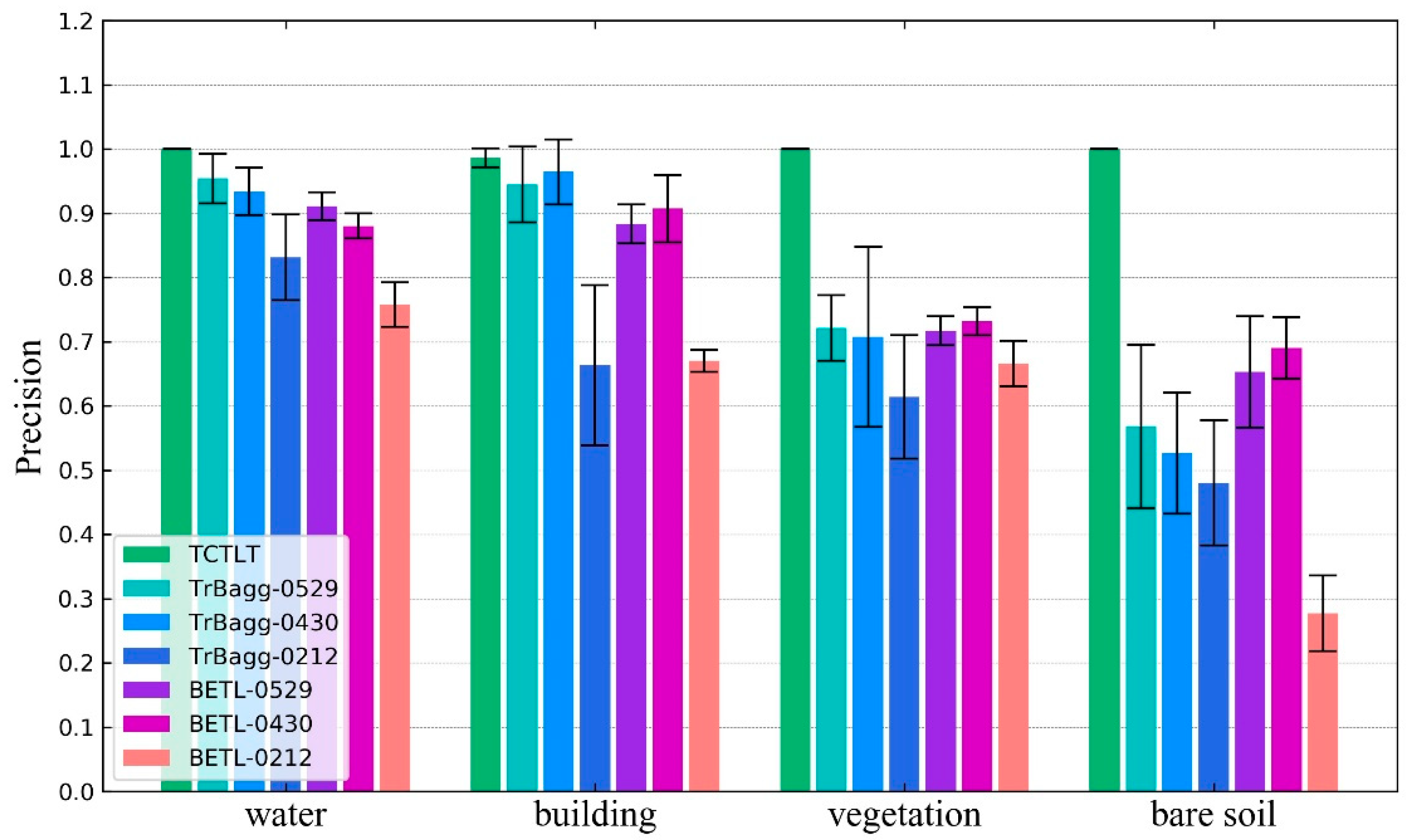
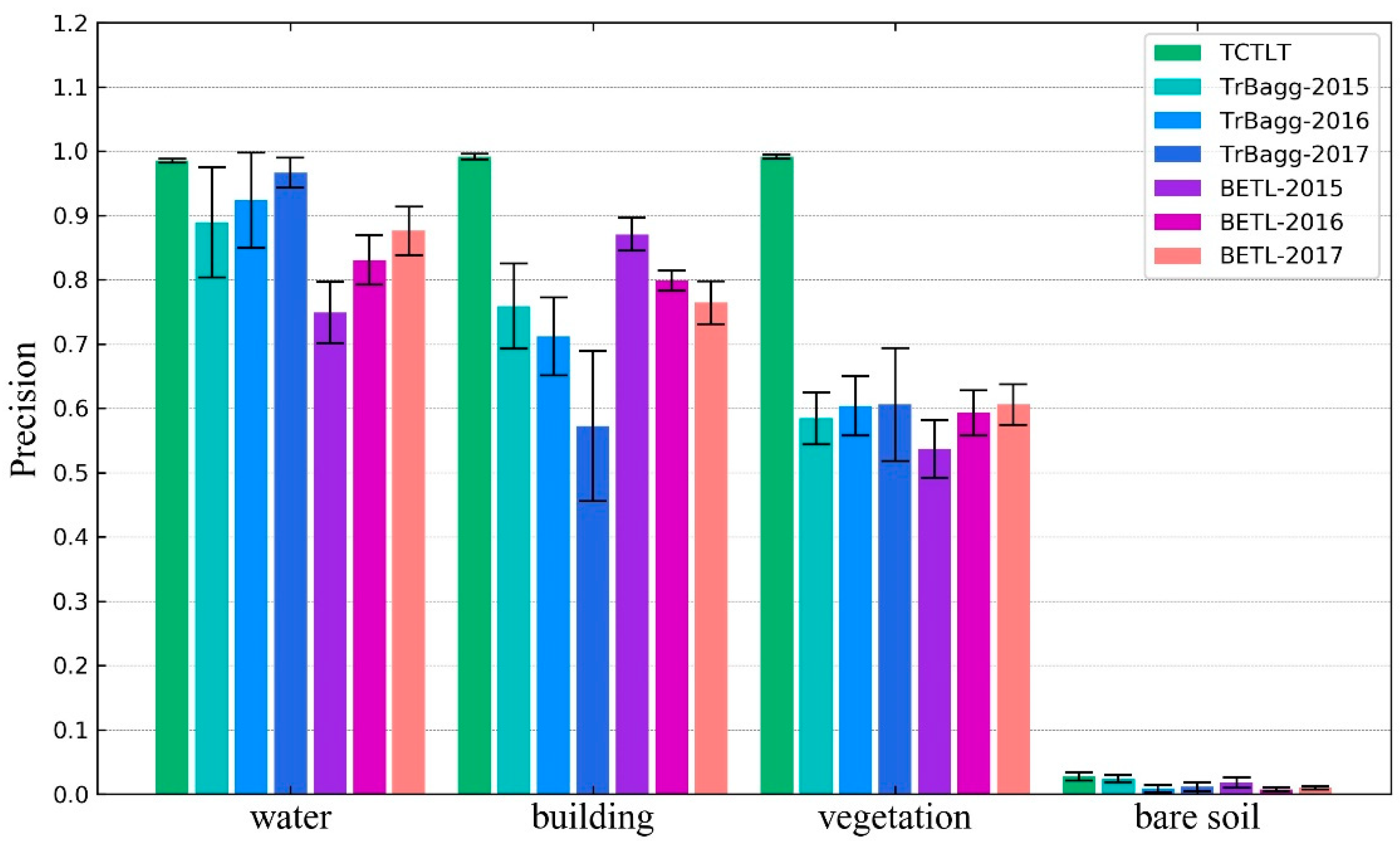
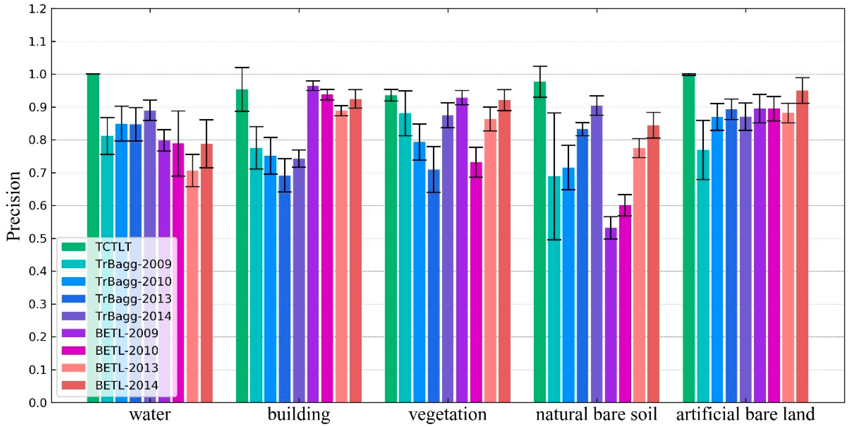
The difference between the target domain and the source domain is an important factor affecting the precision of the transfer learning methods. In this paper, when the difference between the target domain image and the source domain image is large (such as the 0212 image in experiment one), the transfer precision of TrBagg and BETL decreases significantly. Furthermore, for algorithms such as TrBagg and BETL, which rely on integrated weak classifiers for the transfer, the other main factors affecting the precision are the separability of the different classes of ground objects, the performance of the weak classifiers, the selection of features, and the quality of the target domain samples. (1) The transfer precision is high for objects which are easy to classify, but when the object is difficult to distinguish, its transfer precision will be very unreliable. (2) The weak classifier used in the corresponding literature [2,8] was the NB classifier, but in this study, the effect of this classifier was found to be not ideal. After comparing decision tree, NB, and SVM classifiers, it was found that using SVM as the weak classifier could allow TrBagg and BETL to reach a higher precision. (3) Feature selection is an important research topic in image classification and the quality of the feature selection directly affects the classification. In this paper, we do not discuss this issue further, so we chose as many features as possible for TrBagg and BETL. 4) The result of the label transfer is closely related to the quality of the labeled samples in the target domain. Because the labeled samples in the target domain were different in each run of the experiments, the experimental results showed that the transfer precision of TrBagg and BETL varies over a large range (the standard deviation is high).

For the above factors, first of all, the proposed method (TCTLT) is a transfer learning method based on relational knowledge: in a single image, the similarity between the objects of the same class is considered, and in different images, the overall difference is considered. Thus, the proposed method can effectively overcome the problem of a large difference between the target domain and source domain. Secondly, the label transfer process in the proposed method is carried out in a single class of object and is thus not easily affected by the separability of ground objects. Thirdly, this method does not undertake classification, but uses the polarimetric covariance matrix to describe the time-series curve, and designs an effective similarity measure, so that it can obtain reliable time-series clustering results.

TCTLT is also a transductive transfer learning method, which does not need labeled target domain samples in the process of label transfer. Therefore, this method has a high application value. For example, when faced with the classification task for a long time series of images, in the case of existing source domain sample labels, inductive transfer learning methods (such as TrBagg and BETL) need to select a certain number of labeled samples from each target domain image, and the more samples that are selected, the more accurate the transfer will be, so a lot of manual participation is needed. In contrast, the proposed method uses temporal and spatial correlation information between the time-series images to replace the supervised information of the target domain for the label transfer, without additional workload. Therefore, in the case of a long time series and a large amount of data, the advantages of TCTLT are more obvious. Thus, we believe that TCTLT will be able to provide technical support for surface dynamics monitoring, emergency response, remote sensing processing of large data volumes, and so on.

We have also observed the computational efficiency of TCTLT. In this method, optimization clustering and cluster merging are more time-consuming. The processing time of optimization clustering is related to the number of cluster centers (represented by m) and the number of time-series samples (represented by n), i.e., its time complexity is $\mathrm{O}\left(m\ast n\right)$, and the time complexity of cluster merging is $\mathrm{O}\left(m\ast m\right)$, which is related to the number of cluster centers. Taking experiment one as an example, the processing time of TCTLT is 518.9s, while the processing time of Trbagg and BETL are 73.5s and 16.7s, respectively. Although the TCTLT have a lower computational efficiency, it is still meaningful in practical applications for its relying not on the target domain labeled samples.

In summary, many of the existing transfer learning methods have strong universality and wide application scenarios, but in the label transfer of PolSAR time-series images, they either cannot achieve a high accuracy or require additional conditions, and thus have difficulty in meeting the requirements. In contrast, TCTLT is designed for PolSAR time-series images, and has strong pertinence, so it is more effective in the label transfer of PolSAR time-series images. The main disadvantage of TCTLT is that it needs to meet the condition that the number of unchanged time-series samples is dominant, but this condition is easily met in most application scenarios.

5. Conclusions

In order to solve the problems of the insufficient utilization of the information in time-series images and the dependence on manual sample selection existing in many of the current transfer learning methods when applied to information extraction from long time series of remote sensing images, a new three-phase time-series clustering algorithm for PolSAR time-series images is proposed for transductive label transfer. This method can transfer the labels of the source domain samples to the target domain samples, without using the labeled samples of the target domain. Three different groups of PolSAR time-series images were used in our experiments, and two existing transfer learning algorithms were used for a comparison. Thus, the label transfer ability of the proposed method in PolSAR time-series images with different imaging directions, from different sensors, and with complex object classes was well verified. The experimental results showed that TCTLT has strong robustness and effectiveness. It provides a new idea for automatic information extraction from PolSAR time-series images and has a certain practical application value. In our future study, we will attempt to expand the application scenarios of TCTLT and further improve its applicability.

References

1. Pan, S.J.; Yang, Q. A Survey on Transfer Learning. IEEE Trans. Knowl. Data Eng. 2010, 22, 1345–1359. [Google Scholar] [CrossRef]
2. Kamishima, T.; Hamasaki, M.; Akaho, S. TrBagg: A Simple Transfer Learning Method and its Application to Personalization in Collaborative Tagging. In Proceedings of the Ninth IEEE International Conference on Data Mining, Miami, FL, USA, 6–9 December 2009. [Google Scholar]
3. Chattopadhyay, R.; Ye, J.; Panchanathan, S.; Fan, W.; Davidson, I. Multisource Domain Adaptation and Its Application to Early Detection of Fatigue. ACM Trans. Knowl. Discov. Data 2011, 6, 717–725. [Google Scholar] [CrossRef]
4. Duh, K.; Fujino, A. Flexible sample selection strategies for transfer learning in ranking. Inf. Process. Manag. 2012, 48, 502–512. [Google Scholar] [CrossRef]
5. Li, X.; Mao, W.; Jiang, W. Extreme learning machine based transfer learning for data classification. Neurocomputing 2016, 174, 203–210. [Google Scholar] [CrossRef]
6. Lin, D.; An, X.; Zhang, J. Double-bootstrapping source data selection for instance-based transfer learning. Pattern Recognit. Lett. 2013, 34, 1279–1285. [Google Scholar] [CrossRef]
7. Dai, W.; Yang, Q.; Xue, G.-R.; Yu, Y. Boosting for Transfer Learning. In Proceedings of the ACM International Conference Proceeding Series, Corvalis, OR, USA, 20–24 June 2007; pp. 193–200. [Google Scholar]
8. Liu, X.; Wang, G.; Cai, Z.; Zhang, H. Bagging based ensemble transfer learning. J. Ambient Intell. Humaniz. Comput. 2016, 7, 29–36. [Google Scholar] [CrossRef]
9. Wang, Y.; Zhai, J.; Li, Y.; Chen, K.; Xue, H. Transfer learning with partial related “instance-feature” knowledge. Neurocomputing 2018, 310, 115–124. [Google Scholar] [CrossRef]
10. Ben-David, S.; Blitzer, J.; Crammer, K.; Kulesza, A.; Pereira, F.; Vaughan, J.W. A theory of learning from different domains. Mach. Learn. 2010, 79, 151–175. [Google Scholar] [CrossRef]
11. Hu, X.; Pan, J.; Li, P.; Li, H.; He, W.; Zhang, Y. Multi-bridge transfer learning. Knowl.-Based Syst. 2016, 97, 60–74. [Google Scholar] [CrossRef]
12. Oquab, M.; Bottou, L.; Laptev, I.; Sivic, J. Learning and Transferring Mid-Level Image Representations using Convolutional Neural Networks. In Proceedings of the IEEE Computer Society Conference on Computer Vision and Pattern Recognition, Columbus, OH, USA, 23–28 June 2014. [Google Scholar]
13. Dredze, M.; Kulesza, A.; Crammer, K. Multi-domain learning by confidence-weighted parameter combination. Mach. Learn. 2010, 79, 123–149. [Google Scholar] [CrossRef]
14. Tao, J.; Chung, F.; Wang, S. A kernel learning framework for domain adaptation learning. Sci. China Inf. Sci. 2012, 55, 1983–2007. [Google Scholar] [CrossRef]
15. Theckelp-Joy, T.; Rana, S.; Gupta, S.; Venkatesh, S. A flexible transfer learning framework for Bayesian optimization with convergence guarantee. Expert Syst. Appl. 2019, 115, 656–672. [Google Scholar] [CrossRef]
16. Duan, L.; Xu, D.; Tsang, I.W. Domain Adaptation From Multiple Sources: A Domain-Dependent Regularization Approach. IEEE Trans. Neural Netw. Learn. Syst. 2012, 23, 504–518. [Google Scholar] [CrossRef]
17. Wang, D.; Li, Y.; Lin, Y.; Zhuang, Y. Relational knowledge transfer for zero-shot learning. In Proceedings of the Thirtieth AAAI Conference on Artificial Intelligence, Phoenix, AZ, USA, 12–17 February 2016; pp. 2145–2151. [Google Scholar]
18. Zhao, P.; Hoi, S.C.H.; Wang, J.; Li, B. Online Transfer Learning. Artif. Intell. 2014, 216, 76–102. [Google Scholar] [CrossRef]
19. Mihalkova, L.; Huynh, T.; Mooney, R.J. Mapping and revising Markov logic networks for transfer learning. In Proceedings of the 22nd National Conference on Artificial Intelligence—Volume 1, Vancouver, BC, Canada, 22–26 July 2007; pp. 608–614. [Google Scholar]
20. Xiang, E.W.; Cao, B.; Hu, D.H.; Yang, Q. Bridging Domains Using World Wide Knowledge for Transfer Learning. IEEE Trans. Knowl. Data Eng. 2010, 22, 770–783. [Google Scholar] [CrossRef]
21. Aghabozorgi, S.; Shirkhorshidi, A.S.; Wah, T.Y. Time-series clustering—A decade review. Inf. Syst. 2015, 53, 16–38. [Google Scholar] [CrossRef]
22. Kumar, M.; Patel, N.R.; Woo, J. Clustering seasonality patterns in the presence of errors. In Proceedings of the Eighth ACM SIGKDD International Conference on Knowledge Discovery and Data Mining, Edmonton, AB, Canada, 23–25 July 2002; pp. 557–563. [Google Scholar]
23. Liu, S.; Maharaj, E.A.; Inder, B. Polarization of forecast densities: A new approach to time series classification. Comput. Stat. Data Anal. 2014, 70, 345–361. [Google Scholar] [CrossRef] [Green Version]
24. Ngom, A.; Burden, C.J.; Rueda, L.; Subhani, N. Multiple gene expression profile alignment for microarray time-series data clustering. Bioinformatics 2010, 26, 2281–2288. [Google Scholar] [CrossRef] [Green Version]
25. Pyatnitskiy, M.; Mazo, I.; Shkrob, M.; Schwartz, E.; Kotelnikova, E. Clustering Gene Expression Regulators: New Approach to Disease Subtyping. PLoS ONE 2014, 9, e84955. [Google Scholar] [CrossRef]
26. Elangasinghe, M.A.; Singhal, N.; Dirks, K.N.; Salmond, J.A.; Samarasinghe, S. Complex time series analysis of PM10 and PM2.5 for a coastal site using artificial neural network modelling and k-means clustering. Atmos. Environ. 2014, 94, 106–116. [Google Scholar] [CrossRef]
27. Aghabozorgi, S.; Teh, Y.W. Stock market co-movement assessment using a three-phase clustering method. Expert Syst. Appl. 2014, 41, 1301–1314. [Google Scholar] [CrossRef]
28. Corduas, M.; Piccolo, D. Time series clustering and classification by the autoregressive metric. Comput. Stat. Data Anal. 2008, 52, 1860–1872. [Google Scholar] [CrossRef]
29. Chen, Q.; Chen, L.; Lian, X.; Liu, Y.; Yu, J.X. Indexable PLA for efficient similarity search. In Proceedings of the 33rd International Conference on Very Large Data Bases, Vienna, Austria, 23–28 September 2007; pp. 435–446. [Google Scholar]
30. Wang, X.; Mueen, A.; Ding, H.; Trajcevski, G.; Scheuermann, P.; Keogh, E. Experimental comparison of representation methods and distance measures for time series data. Data Min. Knowl. Discov. 2013, 26, 275–309. [Google Scholar] [CrossRef]
31. Wang, X.; Wang, P.; Pei, J.; Wang, W.; Huang, H. A data-adaptive and dynamic segmentation index for whole matching on time series. Proc. VLDB Endow. 2013, 6, 793–804. [Google Scholar] [CrossRef]
32. Bagnall, A.; Ratanamahatana, C.A.; Keogh, E.; Lonardi, S.; Janacek, G. A Bit Level Representation for Time Series Data Mining with Shape Based Similarity. Data Min. Knowl. Discov. 2006, 13, 11–40. [Google Scholar] [CrossRef]
33. Keogh, E.; Knowledge, C.A.R.J.; Systems, I. Exact indexing of dynamic time warping. Knowl. Inf. Syst. 2005, 7, 358–386. [Google Scholar] [CrossRef]
34. Bagnall, A.; Janacek, G. Clustering Time Series with Clipped Data. Mach. Learn. 2005, 58, 151–178. [Google Scholar] [CrossRef] [Green Version]
35. Lauwers, O.; Moor, B.D. A Time Series Distance Measure for Efficient Clustering of Input/Output Signals by Their Underlying Dynamics. IEEE Control Syst. Lett. 2017, 1, 286–291. [Google Scholar] [CrossRef]
36. Sharabiani, A.; Darabi, H.; Harford, S.; Douzali, E.; Karim, F.; Johnson, H.; Chen, S. Asymptotic Dynamic Time Warping calculation with utilizing value repetition. Knowl. Inf. Syst. 2018, 57, 359–388. [Google Scholar] [CrossRef]
37. Panuccio, A.; Bicego, M.; Murino, V. A Hidden Markov Model-Based Approach to Sequential Data Clustering. In Proceedings of the Joint Iapr International Workshops on Statistical Techniques in Pattern Recognition, Windsor, ON, Canada, 6–9 August 2002. [Google Scholar]
38. Keogh, E.; Lonardi, S.; Ratanamahatana, C.A.; Wei, L.; Lee, S.-H.; Handley, J. Compression-based data mining of sequential data. Data Min. Knowl. Discov. 2007, 14, 99–129. [Google Scholar] [CrossRef]
39. Ratanamahatana, C.A.; Keogh, E. Multimedia Retrieval Using Time Series Representation and Relevance Feedback. In Proceedings of the Digital Libraries: Implementing Strategies and Sharing Experiences; Springer: Berlin/Heidelberg, Germany, 2005; pp. 400–405. [Google Scholar]
40. Corradini, A. Dynamic time warping for off-line recognition of a small gesture vocabulary. In Proceedings of the IEEE ICCV Workshop on Recognition, Analysis, and Tracking of Faces and Gestures in Real-Time Systems, Vancouver, BC, Canada, 13 July 2001; pp. 82–89. [Google Scholar]
41. Ratanamahatana, C.; Keogh, E.J. Three Myths about Dynamic Time Warping Data Mining. In Proceedings of the SIAM International Conference on Data Mining, Philadelphia, PA, USA, 20–23 August 2005; pp. 506–510. [Google Scholar]
42. von Luxburg, U. A tutorial on spectral clustering. Stat. Comput. 2007, 17, 395–416. [Google Scholar] [CrossRef]
43. Kersten, P.R.; Jong-Sen, L.; Ainsworth, T.L. Unsupervised classification of polarimetric synthetic aperture Radar images using fuzzy clustering and EM clustering. IEEE Trans. Geosci. Remote Sens. 2005, 43, 519–527. [Google Scholar] [CrossRef]
44. Anfinsen, S.; Jenssen, R.; Eltoft, T. Spectral Clustering of Polarimetric SAR Data with Wishart-Derived Distance Measures. Proc. POLinSAR 2007, 7, 1–9. [Google Scholar]
Figure 1. Examples of different types of water time-series samples. Image 2 is the source domain, while the other images are target domains.
Remotesensing 11 01358 g001
Figure 2. Flow chart of the three-phase time-series clustering algorithm. DVI: Dunn validity index.
Remotesensing 11 01358 g002
Figure 3. The curve of DVI change with merging times. The green line is the DVI, the blue line is the min distance between classes, and the red line is the max intra-class distance.
Remotesensing 11 01358 g003
Figure 4. Pauli RGB images of the first group of time-series images, with red | S H H S V V | 2 , green 4 | S H V | 2 , and blue | S H H + S V V | 2 . The image of 20170824 is the source domain and the other images are the target domain.
Remotesensing 11 01358 g004
Figure 5. The mean and standard deviation curves of each phase. (a) The DVI of each phase. (b) The purity of each phase.
Remotesensing 11 01358 g005
Figure 6. The mean and standard deviation of the label transfer precision of different objects.
Remotesensing 11 01358 g006
Figure 7. Pauli RGB images of the second group of time-series images, with red | S H H S V V | 2 , green 4 | S H V | 2 , and blue | S H H + S V V | 2 . The image of 2011 is the source domain and the other images are the target domain.
Remotesensing 11 01358 g007
Figure 8. The mean and standard deviation curves of each phase. (a) The DVI of each phase. (b) The purity of each phase.
Remotesensing 11 01358 g008
Figure 9. The mean and standard deviation of the label transfer precision of different objects.
Remotesensing 11 01358 g009
Figure 10. Pauli RGB images of the third group of time-series images, with red | S H H S V V | 2 , green 4 | S H V | 2 , and blue | S H H + S V V | 2 . The image of 2008 is the source domain and the other images are the target domain.
Remotesensing 11 01358 g010
Figure 11. The mean and standard deviation curves of each phase. (a) The DVI of each phase. (b) The purity of each phase.
Remotesensing 11 01358 g011
Figure 12. The mean and standard deviation of the label transfer precision of the different objects.
Remotesensing 11 01358 g012