Article

Analysis of the Development of an Erosion Gully in an Open-Pit Coal Mine Dump During a Winter Freeze-Thaw Cycle by Using Low-Cost UAVs

1
Engineering Research Center of Ministry of Education for Mine Ecological Restoration, China University of Mining and Technology, Xuzhou 221116, China
2
Shenhua Baorixile Energy Ind Co. Ltd., Hulun Buir 021000, China
*
Author to whom correspondence should be addressed.
Remote Sens. 2019, 11(11), 1356; https://doi.org/10.3390/rs11111356
Submission received: 7 May 2019 / Revised: 1 June 2019 / Accepted: 3 June 2019 / Published: 5 June 2019
(This article belongs to the Special Issue Monitoring Soil Degradation by Remote Sensing)

Abstract

:
Open-pit coal mine dumps in semi-arid areas in northern China are affected by serious soil erosion problems. The conventional field investigation method cannot ensure a fine spatial analysis of gully erosion. With recent technological and algorithmic developments in high-resolution terrain measurement, Unmanned Aerial Vehicles (UAVs) and Structure from Motion (SfM) technology have become powerful tools to capture high-resolution terrain data. In this study, two UAV Photogrammetry surveys and modeling were performed at one opencast coal mine dump gully before and after a freeze-thaw cycle. Finally, a three-dimensional digital model of the slope of the drainage field was established, and a centimeter-level-resolution Digital Orthophoto Map (DOM) and a Digital Elevation Model (DEM) were created. Moreover, the development process of the erosion zone of the open-pit mine dump during a freeze-thaw cycle was studied by UAVs. The results show that there are clear soil erosion phenomena in the erosion gully of the dump during a freeze-thaw cycle. The erosion degree was different across regions, with the highest erosion occurring in high-slope areas at the upper edge of the bank. Moreover, the phenomenon of flake erosion and “crumble” was recorded. At the same time, the NE-E-SE slope and the high-sunshine radiation zone were seriously eroded. Finally, the relationship between the development process of the erosion gully and micro-topography factors was analyzed, providing managers with a sound scientific basis to implement land restoration.

Graphical Abstract

1. Introduction

The snow-thaw runoff of diurnal and seasonal permafrost is the main geomorphic agent in cold, high-latitude and high-altitude regions [1,2,3,4]. Seasonal fluctuations in circulation and temperature lead to daily fluctuations in soil, resulting in the thawing of permafrost and ice, which can significantly alter soil erosion [5]. Meltwater is more conducive to soil erosion than rainfall in both mid- and high-latitude upland watersheds [6] and threatens soil and slope stability [7,8].
Previous research has focused on the development of gully erosion on natural landforms [9,10], while man-made landforms (e.g., open-pit mining dumps) have been neglected. In northern China, hundreds of labile, gully filled open-pit coal mine dump fields are surrounded by natural steppe. Here, open-pit mining has caused severe disturbances to the mine field; moreover, the dumping sites, containing a large amount of peeling material, are barren and characterized by high slopes (usually up to 100 m), loose slopes and soil compaction platforms, complex material composition, and uneven subsidence [11]. This leads to the destruction of vast amounts of vegetation communities [12] and to an extremely serious risk of soil erosion [13]. Gullies caused by freeze-thaw erosion and meltwater erosion have severely eroded the soil in the dump, inducing slope stability of the dump and sedimentation (one of the most harmful [14,15]) of surrounding grassland [9,16,17,18]. To understand the dynamics of gully erosion, it is necessary to perform an accurate measurement of soil erosion during a freeze-thaw cycle; in this way, it is possible to provide a basis for both land management, and soil and water conservation management.
Land managers should be able to choose effective erosion control measures. For this purpose, gully erosion should be analyzed quantitatively. The method of gully extraction relies on the collection of geographic data. The most traditionally used methods are simulation experiment [19], field surveys [20,21], 137Cs approach [22], and numerical simulations [23], which is extremely complicated, time- and resource-consuming work. Existing erosion modeling studies include applications and adaptations of simple empirical models, such as the Universal Soil Loss Equation (USLE) [24] and its revised version, the RUSLE model [25]. The ‘vertical column’ representation, used in the geomorphological continuity equation, is generally applicable to the vertical variation of the surface height, but not to the horizontal movement of steep surfaces such as steep slopes and riverbanks [26]. Over the past decade, the advances in remote sensing technologies have greatly facilitated the mapping and quantification of soil erosion processes [10,27,28,29,30].
With the development of unmanned aerial vehicles (UAVs) and sensors, the technology of low-altitude (<1000 m) photogrammetry based on UAV platforms has shown its unique superiority. UAV Photogrammetry has the feature of automation; moreover, it has the advantages of a flexible system, convenient take-offs and landings, low cost, and high imaging quality. In addition, it can rapidly cover small areas, while at the same time cover difficult flight areas and provide high-resolution images of complex terrain areas. As such, it has rapidly become a complement of both field surveys and satellite and aircraft remote sensing [31].
At present, the UAV Photogrammetry technology has been widely used in topographic surveys [32], environmental monitoring [33,34], vegetation information extraction, coastal zone extraction [35], precision agriculture [36], glacier dynamics [37], landslides [38], cultural relics protection [39], and building risk assessment [40]. In addition, thanks to the use of multiple flights and of single tilt-shift lenses to improve data accuracy, the spatial information density and accuracy of UAV Photogrammetry can be compared with that of airborne LiDAR and TLS [41,42]. Several authors have adopted centimeter-level precision, high-resolution Digital Surface Model (DSMs) volume estimation, erosion rate measurement, morphological analysis, and trench monitoring from UAV image calculations [31,43,44]. In this study, we employed a low-cost quadrotor to perform both a multi-temporal DoD calculation and a micro-topography change detection at a hillslope in an open-pit mine dump. Furthermore, we estimated the erosion of the study area during a winter freeze-thaw cycle and the relationship between the degree of erosion and the micro-topography of the area.
The majority of existing gully erosion studies have focused on runoff erosion during the rainy season [45], while neglecting meltwater erosion. Therefore, the purpose of this paper is to investigate the effects of meltwater erosion on gullies during the winter season. We acquired data by using oblique photography and developed a comprehensive 3D model of the gully to quantify the amount of erosion produced in the gullies. The study was performed in the Baorixile open-pit coal mine dump site in Hulunbeier, China.

2. Materials and Methods
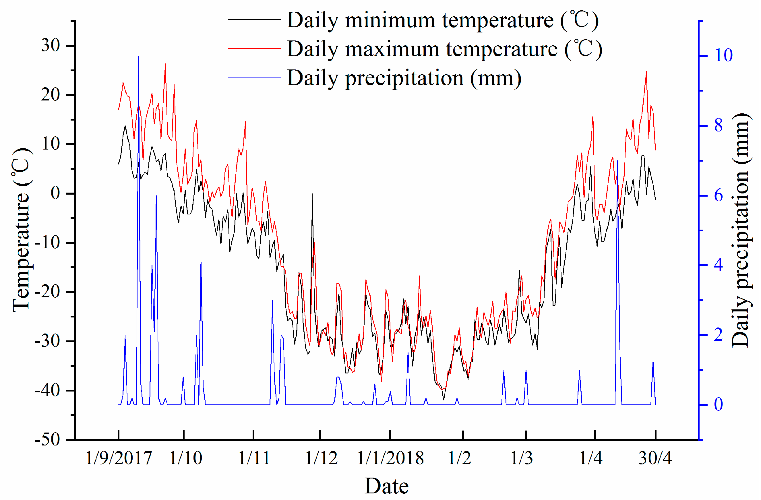
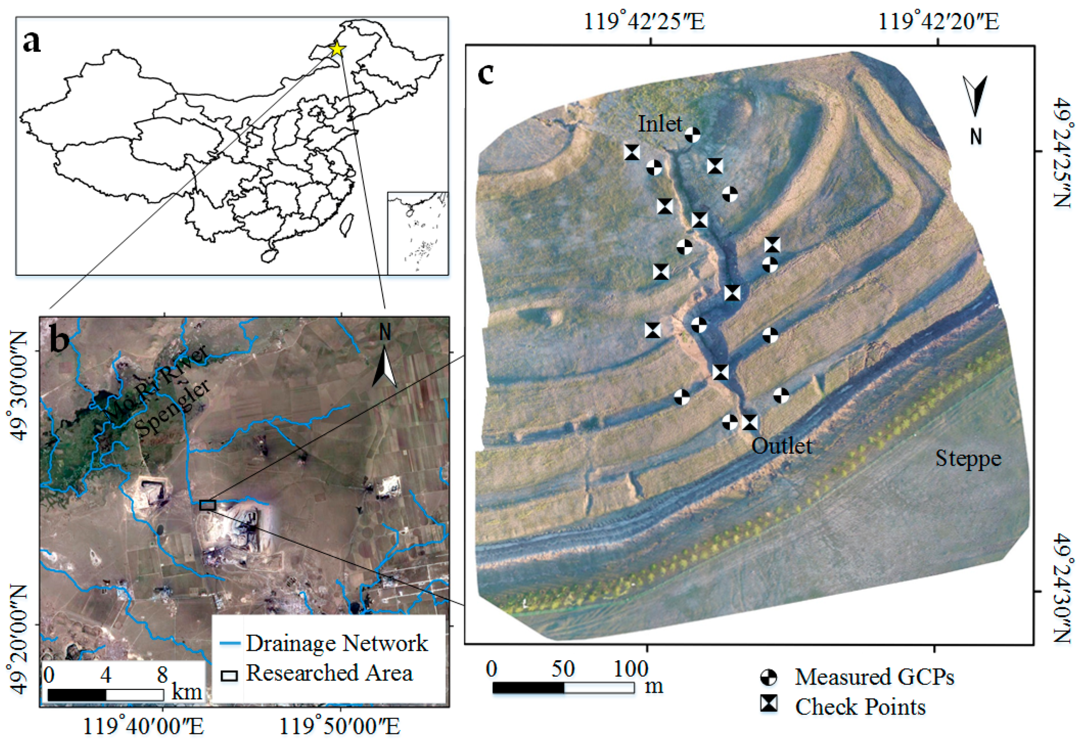
2.1. The Study Area

The study site (119°41ʹ25ʺ E, 49°24ʹ29ʺ N) is located in the northeastern part of Inner Mongolia, in China (see Figure 1). This region has a temperate continental monsoon climate. The average annual temperature is between −2.4 °C and 2.2 °C, while the highest and lowest temperatures recorded are 17 °C and −48.5 °C, respectively. The frost-free period is usually 100 to 120 days long; in the period 2009–2018, the average annual precipitation was 371.5 mm (with 70% of the rainfall recorded in August), while evaporation was 1247 mm [46]. During the study period (from October 2017 until May 2018), the cumulative precipitation was about 70.9 mm in the form of snow, with an average temperature of −8.3 °C.
Because of soil properties, precipitation behavior, and land use characteristics, the dump is especially prone to high erosion rates, and gullies are a frequent phenomenon. Additionally, the high erosion of dumps can be attributed to their geochemical properties (e.g., high concentrations of montmorillonite), resulting in the dispersion and expansion of soil after rainfall. Table 1 presents the properties of the soil in the 0–20 cm layer of the experimental hillslope. In addition, soil with a high infiltration rate is more susceptible to erosion and formation of gullies under the action of freezing and thawing [6,7,47].
The study site is part of a series of gullies, among which there is a huge gully (see Figure 1c) located at the northern slope of the dump, adjacent to natural pastures. In addition, the length of the headcut is about 120 m, and it is characterized by a maximum width of 3.5 m and a maximum depth of 7.2 m, with both U-shaped and V-shaped sections.
To improve the characterization of the climate of the study site, we obtained the 2017–2018 winter climate diagram (see Figure 2) using data derived from a portable climate station located at a distance of 0.8 km from the study site. Figure 2 displays the daily highest and lowest temperatures and precipitation over a winter freeze-thaw cycle. Two surveys phased at the same soil surface temperature of about 15 °C, to ensure that the soil had the same thermal expansion & contraction.

2.2. Data Acquisition and Processing

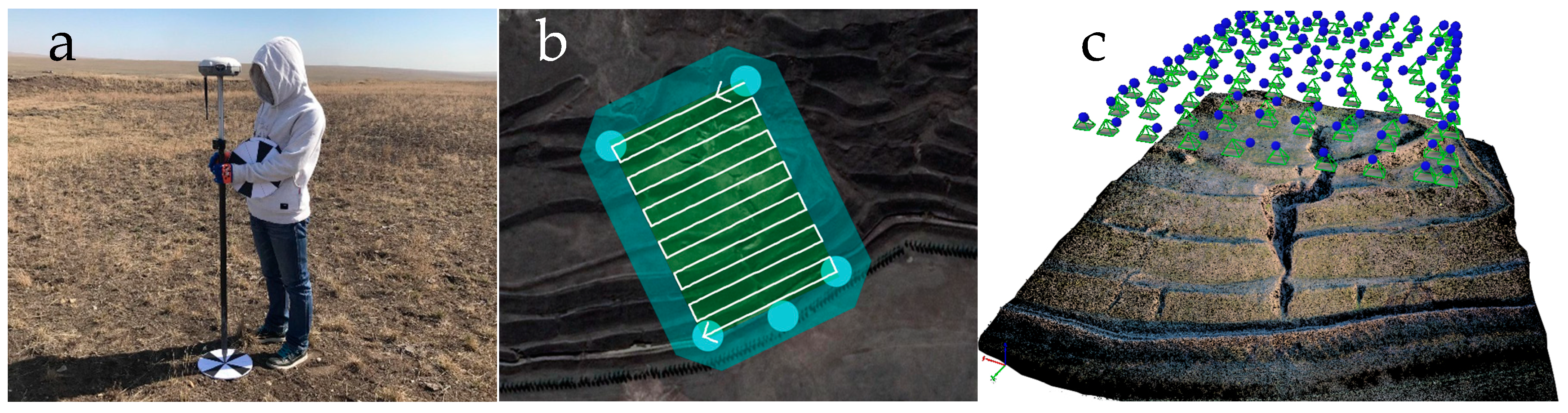
2.2.1. The Reference System

The two seasons (Autumn 2017 and Spring 2018) of the plot were measured using UAV Photogrammetry to derive point cloud representations of the soil surface. Thereby, a reliable and stable reference system is an important prerequisite.
Ground Control Points (GCPs) (black-and-white plastic sheets with a diameter of 20 cm) were positioned both around the gully and inside the gully. The GCPs were assumed to be stable during both survey phases (about 2 hours for each) (see Figure 1c). The GCPs and some random validation points, used to evaluate the accuracy of the MultiView-Stereo (MVS) topographic models, were measured using a CHC X91 Real Time Kinematic GPS (RTK GPS) receiver (see Figure 3a). A total of 10 GCPs were used as ground reference during the SfM processing, and 10 average distribution locations were used as check points (see Figure 1c) to ensure that the overall accuracy can meet the requirements. As already mentioned with respect to the reference system above, the number of GCPs was sufficient during both campaigns.

2.2.2. UAV Imaging Surveys

The land surface was captured via aerial images acquired with a UAV-based camera. We used the micro-drone “DJI Phantom 3 Pro (4k)” (see Table 2), manufactured by Da-Jiang Innovations Science and Technology Co., Ltd. (trading as DJI), with a unit cost of production of approximately US $937. The quadrotor was equipped with an active stabilizing camera cradle head, which ensures sharp images and predefined surface coverage, to compensate for the UAV vibrations and the wind-induced tilt.
The flight plans were programmed along exactly the same route using the Altizure software (v3.2.2 in the first survey phase and v4.2.4 in the second survey phase, see Figure 3b), to ensure a reasonable degree of overlap and flight altitude (see Table 2). A total of five flights were performed to acquire data from various angles (pitch angle 0°; tilt angle 45°) to avoid the doming effect [48]. Each flight had an effective duration of about 20 min (excluding takeoff and landing), and an average speed of 3.5 m/s. The takeoff altitude of UAV is 30 m above ground level. Due to the undulation of terrain, the ground height of the UAV is not constant during the surveys. The camera focal length was set to infinity in all flights to ensure the greatest possible sharpness and depth of focus (see Table 2).
Therefore, we used UAVs to conduct field surveys of the gully of the dump site in the open-pit coal mine. The aerial survey campaign was conducted between 1 October 2017 and 1 May 2018. All flights (5 * 2 missions) were performed within a 6-h window around the solar zenith to guarantee relatively constant lighting conditions.

2.2.3. Photogrammetric Post-Processing

The headcut was recorded by 957 images in the field campaign of October 2017, and 1132 images in the field campaign of May 2018 (see Table 3). The number of images in May 2018 was higher due to the higher coverage of the second survey. The images were processed with the Pix4Dmapper Pro 3.2 (Pix4D, Lausanne, Switzerland) software to obtain 3D information (i.e., digital elevation models (DEMs)) from 2D images. This software integrates computer vision techniques with photogrammetry algorithms (i.e., an adapted structure-from-motion (SfM) and multi-view stereo matching (MVS) workflow) to obtain high accuracy in aerial imagery processing [49,50]. We applied this method following three main processing steps. First, we computed the key points on the image and used them to find the matching relationship between the images. Then, we estimated the position and the direction of the camera, and computed the 3D coordinates of the matching image point with an iterative bundle block adjustment (BBA), using the previous image matching information. Finally, we generated a dense point cloud (see Figure 3c) and obtained a highly detailed digital surface model [10,51].
UAV Photogrammetry is unable to directly distinguish vegetation from the earth’s surface, and this can be mitigated by using slope detection algorithms and statistical outlier removal (SOR) filters [52]. The majority of the gullies of the dump site were in arid and semiarid regions with sparse vegetation. Moreover, the two sets of data were collected in late autumn and early spring, when the gully masses were bare. Therefore, extra effort was not required to filter vegetation when the photogrammetric processing of UAV data was performed.

2.2.4. Computation of Soil Erosion and Deposition

We investigated erosion and sedimentation patterns using two periods of small-catchment DEMs, and assessed the 8-month net topographic change during the surveys. To calculate the topographic changes between the two survey phases, a DEM of Difference (DoD) was created by subtracting the old DEM from the new DEM, where negative values indicate a decrease in terrain (i.e., erosion), while positive values represent sedimentation. To consider DoD uncertainties, a minimum threshold of detection was applied to distinguish real topographic change from artifacts arising from errors and uncertainties.
The error and terrain uncertainty of each DEM are important indicators to control landform changes. In this study, the minimum detection threshold was used to distinguish between actual terrain changes and errors and uncertainties in the two DEMs. According to the method developed by Taylor [53] and implemented by further studies [54,55] assuming a non-normal distribution, the accidental errors in digital terrain model (DTMs) were propagated into the DoD according to the following equation:
U crit = t ( δ z n e w ) 2 + ( δ z o l d ) 2
where Ucrit is the critical threshold error in the DoD, or Level of Detection (LoD) of significant elevation change; t is the critical t value for a given confidence interval; and δznew and δzold are the standard deviation of the error in the new (May 2018) and the old (October 2017) DTMs, respectively.
Based on quantitative repeatability errors, the 90% confidence interval was used as a statistical threshold to differentiate between DTM model errors and actual surface variations. The critical threshold error of each DoD raster cell was calculated with Equation (1) to derive a LoD, which was eventually subtracted from all DoD cells to derive elevation change maps and calculate the volumes of erosion and deposition.

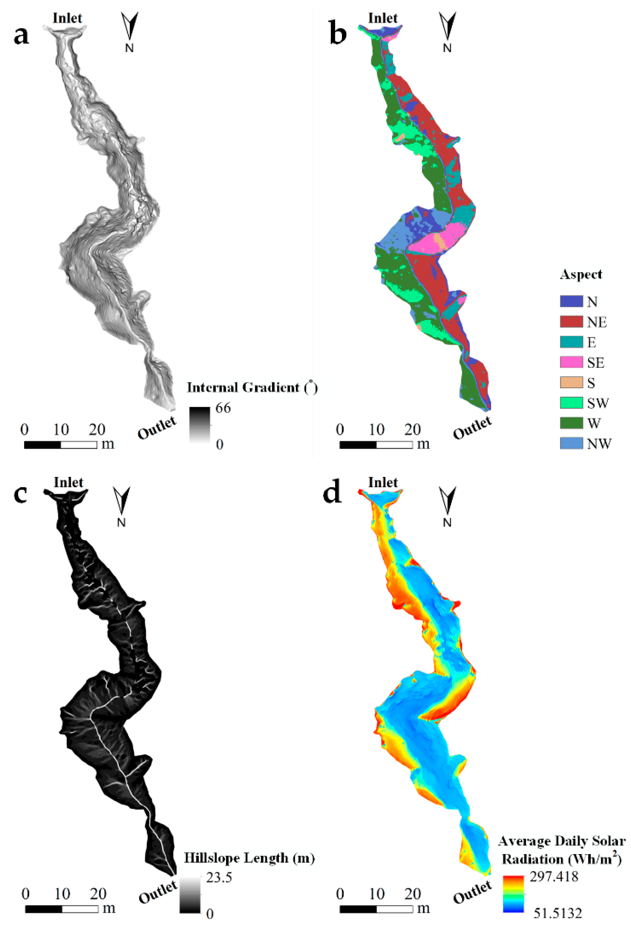
2.2.5. Geomorphometry

We included surface landforms in the geomorphometric analysis performed, and then compared them to the estimated changes of DoD. To further analyze the factors affecting gully erosion and deposition during a winter freeze-thaw cycle, we calculated the relationship between internal gradient, slope orientations, LS factor (L = slope length factor, S = slope steepness factor) [56], average daily solar radiation [57,58], and erosion/deposition of each pixel in the study area. Furthermore, we performed the statistical analysis of the relationship between erosion/deposition on the one side, and other factors on the other side (slope aspect and average daily solar radiation), which was then combined with the erosion and deposition pattern derived from the DoD analysis (see Figure 4a).

3. Results

3.1. Accuracy of the Techniques

The photogrammetric processing produced by the grid DSM provides a ground sampling distance of 1.8 cm. After the processing of the photographic measurements, an accuracy assessment of the data was performed. The accuracy of the three-dimensional coordinates of the DEMs was assessed by comparing the image coordinates with both GCPs and independent check points. We considered all directional vectors to calculate the root mean square error (RMSE). To evaluate the accuracy of the final position in the geometric model, the checkpoint coordinates were located in the orthophoto images and in the DEM using ArcGIS 10.2. Since the ground data mainly show the elevation of the steep groove wall, when measuring checkpoint coordinates in a three-dimensional point cloud, all checkpoint deviations were calculated based on direction (Easting/Northing/Elevation). The GCPs RMSE of easting, northing, and elevation was 0.8 cm, 0.9 cm, and 1.1 cm in October 2017, and 0.5 cm, 0.7 cm, and 1.7 cm in May 2018, respectively. The check points RMSE of easting, northing, and elevation was 1.1 cm, 1.5 cm, and 1.6 cm in October 2017, and 1.3 cm, 1.6 cm, and 1.5 cm in May 2018, respectively (see Table 3).

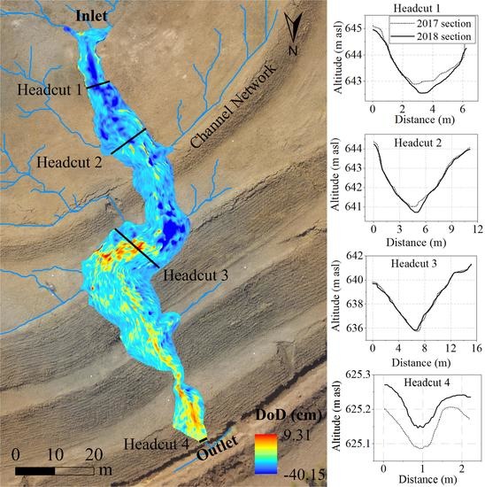
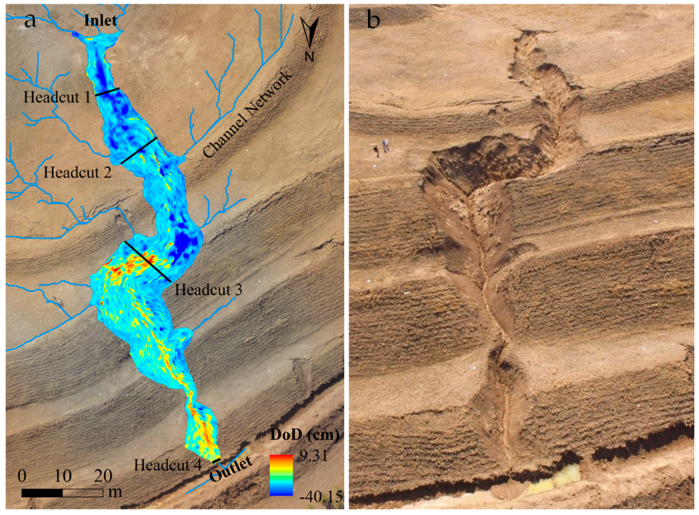
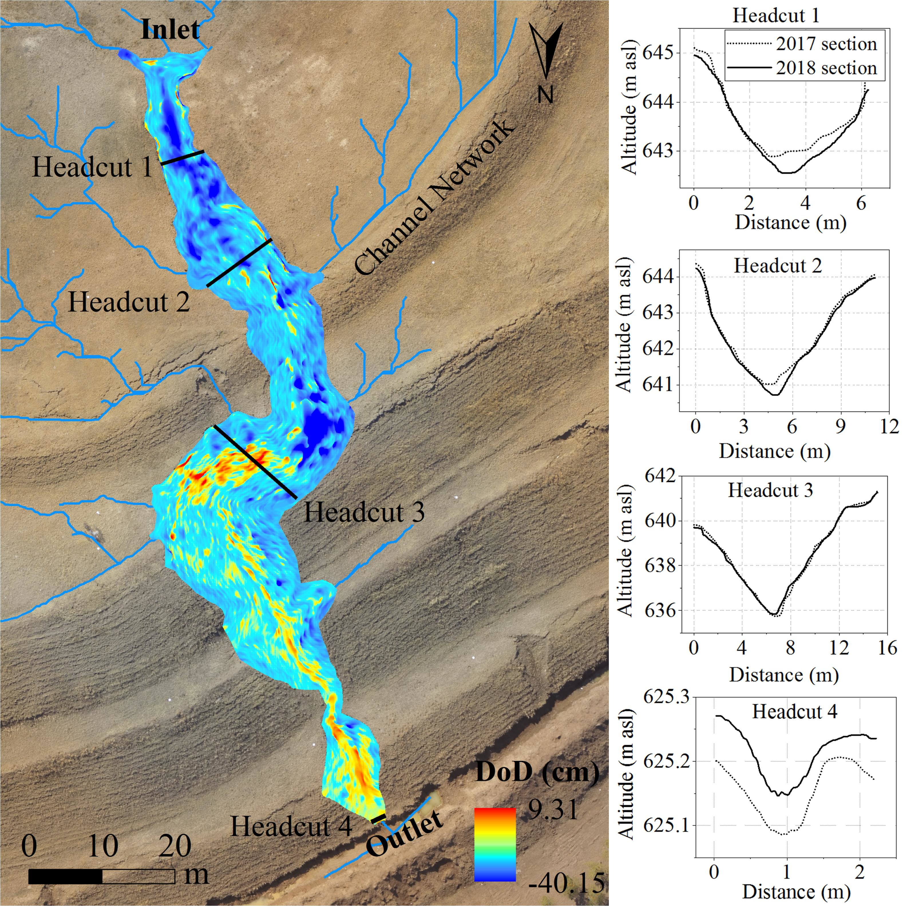
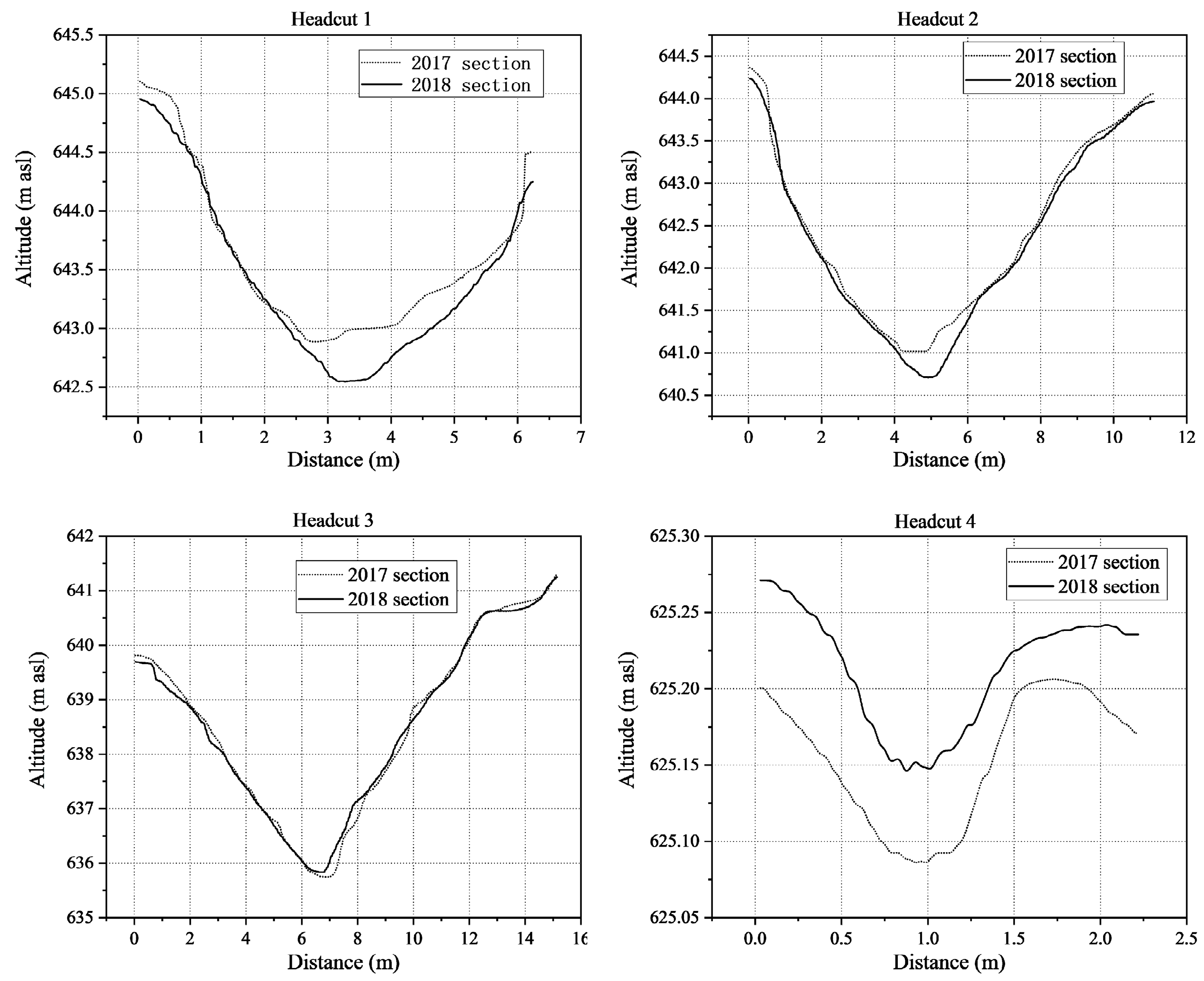
3.2. Characteristic Parameter Extraction

Based on the two survey phases, a high-resolution change detection was performed. ArcGIS 10.2 and ENVI 5.1 were used to extract and statistically analyze gully erosion parameters both before and after winter (see Figure 5, Figure 6, Figure 7 and Figure 8). Clear differences between October and May were recorded in representatively selected headcut profiles (see Figure 5).
For both campaigns, it was not possible to clearly assign the headcuts to a V-shaped morphology, with a homogeneous and almost constant inclination of the walls as well as a narrow gully bed (see Figure 5).
The main slope aspect of the study area was W-WSW and NE-ENE (see Figure 6b and Figure 7b), since the V-shaped gully is located on the northern slope of the dump. As shown in Figure 7a, the average internal gradient of the study area showed a normal distribution from 0° to 66°, a hillslope length in the range between 0–23.5 m (see Figure 7c), and an average daily solar radiation per unit area between 91.51 and 297.42 Wh/m2 (see Figure 7d). In the gully erosion, the altitude difference between the inlet and the outlet was 20.33 m (see additional information in Table 4).

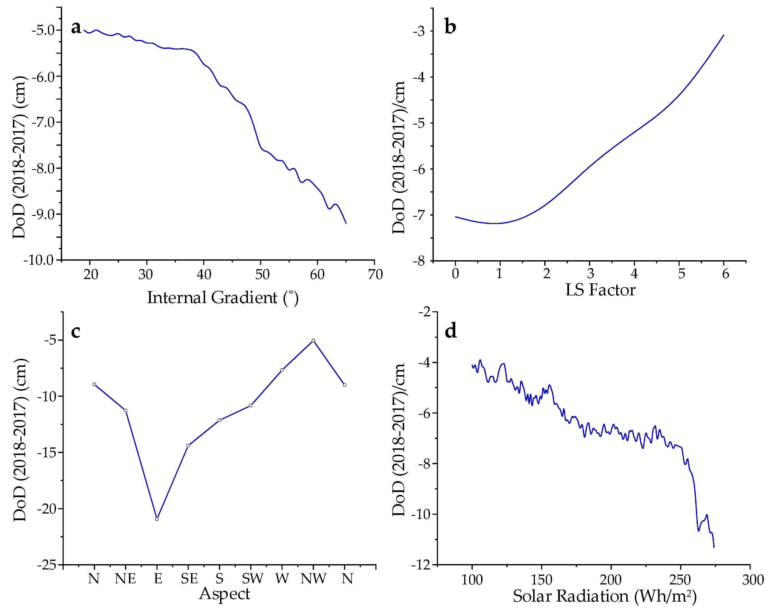
3.3. Relation between Geomorphometry and Geomorphic Changes

The DoD map illustrated in Figure 4 show different spatial patterns of geomorphic change in the study area.
In gullies’ sediment source areas, the elevation differences recorded range from −58.33 cm in 2018 to 7.31 cm in 2017. Positive values represent deposition (i.e., the erosion capacity decreases along the flow line), while negative values indicate erosion (i.e., the erosion capacity increases along the flow line). The gully upstream and midstream are characterized by widespread erosion, while the gully downstream is characterized by deposition (see Figure 4a). Analyzed from the bank perspective (on or near the bottom of the gully), the erodibility of the gully decreases with the distance from an alluvial fan formed at the outlet of the gully (see Figure 4b). Overall, erosion and deposition areas cover 81.0% and 15.7% of the analyzed surface, respectively, while a small area of landform was left unchanged. Besides the spatial pattern, the volumetric change distribution clearly displayed a peak in correspondence with low-magnitude erosion values (see Figure 6a). It can be observed that the elevation change value is close to 0 with a relatively high amplitude of lost information, which is due to the application of the DoD threshold (2 cm) to evaluating uncertainty, as described in Section 2.
We used the DoD analysis to estimate also the sediment yield in the gully during the two surveys. To determine the amount of sediment produced, the total erosion volume obtained from the DoD was subtracted from the volume of the sediment in the gully. The output of the sediment in the gully was calculated, and was then divided by the gully area and by the number of years between the two UAV surveys. We calculated a total sediment yield of about 111.24 m3 and an average sediment yield of 0.117 m3 m−2 at the study site
The relationships between geomorphic changes on the one side, and internal gradient, orientations, hillslope length, and average daily solar radiation per unit area on the other side, were analyzed to obtain the volumetric quantification of sediment transfer (see Figure 8). It is evident that the pattern of erosion-deposition, as detected by the DoD analysis, differs across topographic settings, reflecting their different spatial relationship features. The relationship between erosion/deposition and geomorphological features was statistically differentiated by distinguishing the study area from other sedimentation areas (see Figure 8).
As the internal gradient rises, the degree of soil erosion rises (see Figure 8a). In the area with relatively low slopes (0–40°), the degree of erosion increased slowly. At the same time, in relatively high slope areas (more than 40°), as the slope rises, the degree of erosion increases consistently. With the increase of the LS factor (see Figure 8b), the DoD shows first a feeble decline (corresponding to a LS factor value between 0 and 1) and then a continuous ascent trend (with a LS factor value higher than 1).
There were significant differences in the erosion degree between different slope profiles (see Figure 8c). The NE-E-SE direction was the most eroded (13.93 cm, on average), while the degree of soil erosion gradually decreased from the East direction to the Northwest direction. The NW direction had the lowest degree of erosion (with an average value of 5.05 cm). The northwest slope faced the lowest degree of soil erosion (with an average value of 5.05 cm). Soil erosion was also correlated with the average daily solar radiation per unit area (see Figure 8d).

3.4. Correlations between Explanatory Factors

To correctly analyze the factors that affect the intensity of erosion/deposition processes, it is necessary to understand the interrelationships between explanatory factors; the correlation matrix is shown in Table 5.
The relations between variables was measured with the Pearson-correlation coefficient r. The significance of these coefficients was tested at different probability levels (p) by F-tests. To avoid multicollinearity in multiple regressions, correlation matrices were established between the independent variables. Moreover, the Principal Component Analysis (PCA) was used to reduce the dimensionality of a highly dimensioned data set and simplified the analysis process. Analysis was performed using Statistical Package for Social Sciences (SPSS) version 25.0. Stepwise multiple linear regression was applied for soil erosion, including the most significant explanatory variables, typically have the following format:
DoD = 0.041 x 1 0.016 x 2 1.69     R 2   =   0.96
where DoD is topography change by DEM2018 minus DEM2017; and x1 and x2 are the internal gradient and the daily solar radiation of the study area. The DoD is usually negative, and the greater its absolute value, the greater the erosion.

4. Discussion

4.1. The Quality of UAV-Based Topographic Surveys

UAV surveys combined with GCPs can provide a robust and consistent, high-precision database for the study of gully morphology. The combination of orthophoto and oblique photography for data acquisition is used to the greater range of perspectives and to reduce the doming effects arising by inaccurate camera models. Data accuracy is comparable with that of the TLS-derived DEM [59] for the following reasons: (i) the UAV Photogrammetry can usually collect valid data more efficiently than TLS; (ii) the sub-grid roughness of the SfM-MVS dataset is generally lower; and (iii) the SfM-MVS provides an improved data perspective (i.e., smaller shadows). Because high-resolution terrain data can be obtained at plot scale, and the details of individual debris are clearly visible, the SfM-MVS is perfectly capable of detecting terrain changes and sediment budgets, and even to track the motion of single debris. This computer vision application has shown promising results in studies by other scholars such as Smith et al. [60], who successfully reconstructed 3D high-resolution gully monitoring, and Kaiser et al. [61], who structured complex gullies, both of whom used motion (SfM) techniques. Moreover, in this context the combination of UAVs, LiDAR, 3D laser scanners, and InSAR has recently become a new trend [59,62].
The morphological measurement of sediment budgets requires also a distinction between erosion/deposition and surface shrinking/swelling (e.g., expansive soil, see Table 1), which in turn requires additional datasets such as deep anchor ground control points, or more frequent data collection. In addition, morphometric surveys of sediment budgets require also a differentiation between the topographic changes caused by soil erosion/deposition and by soil shrinking/swelling, which in turn requires additional data sets (i.e., a more frequent data collection combined with deep-anchored ground control points). Moreover, a critical threshold was applied in this study to filter out small changes in the DoD that could not be affirmed as true values (i.e., different from errors). This filtering process can discard a large number of tiny terrain changes [63]. As a result, the DoD analysis may underestimate erosion and deposition. However, this change was minimal by definition, and therefore this effect did not lead to significant deviations in the estimated sediment yield.

4.2. Relationships between Topographic Changes and Geomorphometric Parameters

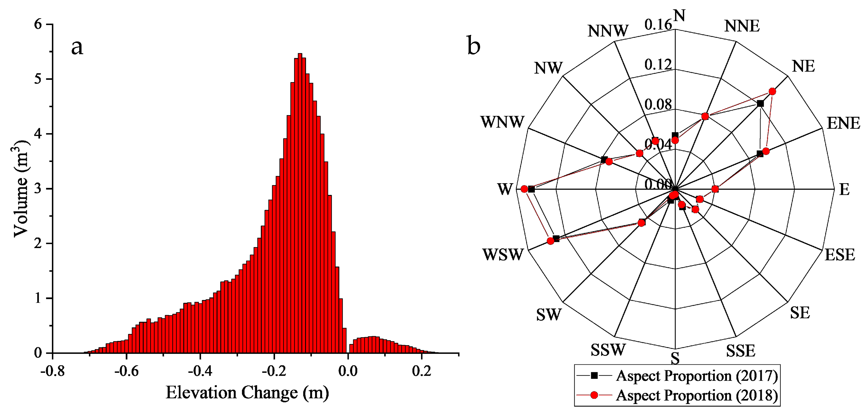
4.2.1. Distribution of Erosion/Deposition

The slope of the gully erosion of the dump site is a type of water erosion (or meltwater erosion) landform occurring in the snowmelt season. Local catchment, infiltration, and freezing-thawing have effects on the development of the gully erosion. In the study area, erosion occurred mainly in the upper and middle parts of the gully bank and in the upper reaches of the gully bottom, while sedimentation began to appear downstream in the bottom of the gully (see Figure 4 and Figure 5).
The occurrence of a geomorphological unit’s erosion/deposition is affected by the slope degree and slope type, which determine runoff velocity to a great extent. Moreover, sediment collection in runoff is a dynamic process [64,65]. Artificially stacked open-pit mine dump fields are loosely earthy and can be easily transported under snowmelt erosion; this allows the sediment concentration along the gully to reach saturation within a short runoff length. A slight drop in flow rate (e.g., due to terrain slope drops or to the increasing roughness of the local terrain) results in a smaller capacity to carry sediment concentration, and in deposition instead of erosion [66].
The worst erosion occurred on the hottest afternoon recorded. Meltwater flows erode riverbeds and carry the maximum sediment concentration under given hydrological conditions. As the temperature rises, both the melt depth of the permafrost and meltwater increase. A higher meltwater flow transports a higher quantity of eroded sediments, leading to more severe erosion on steeper slopes. However, thawed topsoil may freeze and the flow of melted water may stop [67]. During the freeze-thaw season, the meltwater runoff stopped and started again the next morning, erosion temporarily stopped at night.
In addition to the local effects of other variables, the dominance of sheet erosion on the NE-E-SE slope aspect can be directly related to the greater precipitation (or snowfall pattern) that these slopes receive, due to dominant wind directions.
In comparison, there is a high correlation between the average daily solar radiation per unit area and soil erosion. The average daily solar radiation per unit area considers the effects of atmospheric agents, the latitude and the elevation of the site, the steepness (or slope) and the compass direction (or azimuth), the daily and seasonal variations of the solar angle, and the shadows projected by the surrounding terrain. In low radiation areas (90–135 Wh/m2), the rate of soil thawing increases with the increase of radiation volume. The water flowing on permafrost with thawing soil has a high speed and a much lower friction resistance than soil, with the result being that higher flow rates carry a higher quantity of sediments. High radiation areas (136–296 Wh/m2) are mainly concentrated in the south slope, where erosion rate is low due to the main wind direction.

4.2.2. Construction of the Erosion Rate Model for Different Slopes

The comparison between the factors influencing the gully suggests that soil erosion is strongly correlated with the internal gradient, and occurs mostly on the slopes exposed to the east. It is also often associated with the hillslope length and the average daily solar radiation per unit area.
The area with relatively low slopes is mainly located in the bottom part of the gully bank; here, soil erosion is greatly affected by slope length. In parallel, the long hillslope area is less eroded or subject to deposition. Because the phenomenon of slope confluence will increase with the increase of slope length, resulting in the increase of runoff thickness, the increase of the sand carrying capacity will reduce the denudation quantity. Consequently, the growth of the slope length will not increase significantly the erosion capacity in the downstream of the gully. With the further increase of the slope length, when the sediment carrying sand energy reaches a certain upper limit, the erosion intensity of runoff reaches the upper limit, after which the erosion capacity decreases with the increase of the slope length, and the sedimentary phenomenon occurs [68,69].
High (>60°) slope areas with a small size, corresponding to 2% of the total, and strong erosion, are mainly located in the upper edge of the gully bank. This area is near the snowmelt line. Under daytime heat, the snow melts and seeps into the soil; when the temperature drops at night, the snow water freezes and expands, causing the soil to disintegrate and break. It is easy to form tensile fissures at the top of the gully bank and prone to "crumble" and flake during the freeze-thaw cycle. Erosion of the gully bank will develop outward, so that the erosion gully becomes integrally wider, while during the rainy season only the linear erosion of the runoff rill will occur.

5. Conclusions

A spatial analysis (including the geomorphometry analysis and the hydrological analysis) of the erosion gully of the dump was performed using the centimeter-resolution DEMs obtained by the UAV. The measurement of the amount of erosion in the gully by using conventional measurement methods may be an extremely complicated, time- and resource-consuming work. The use of UAVs and SfM technologies may significantly improve productivity and measurement accuracy. Using 3D and GIS spatial analysis technologies, it may be easy to obtain the characteristic parameters of the typical erosion gullies of open-pit mine dumps. By performing a statistical analysis of the slope, slope length, LS factor, aspect, and average daily solar radiation of the erosion gully, as well as a regression analysis with the erosion degree, a high causality was found in this study between the erosion degree on the one side, and slope and average daily solar radiation on the other side, during a freeze-thaw cycle.
This study showed that significant improvement to measurement efficiency and accuracy can be achieved by augmenting traditional soil loss and runoff measurement with 3D surface change information. High-resolution DEM can show the fragile areas of erosion and development of the drainage field during a freeze-thaw cycle. Both UAV and SfM technologies provide a solid basis for the establishment of a freeze-thaw erosion model of soil gully erosion, which is of great significance to monitor the development of surface erosion.

Author Contributions

Conceptualization, C.G.; methodology, C.G. and S.L.; validation, S.L.; formal analysis, C.G.; investigation, C.G., Y.L., W.C. and Z.Z.; writing—original draft preparation, C.G.; writing—review and editing, Z.B. and S.L.; supervision, Z.B. and S.L.; project administration, S.L.; funding acquisition, S.L.

Funding

This research was funded by National Key Research and Development Program of China, grant number 2016YFC0501107.

Acknowledgments

We thank the editor, Traey Wu and three anonymous reviewers for their constructive suggestions. Thanks are due also to the Shenhua Baorixile Energy Ind Co. Ltd. for the provision of the basic data.

Conflicts of Interest

The authors declare no conflict of interest.

References

  1. Johnsson, H.; Lundin, L.-C. Surface runoff and soil water percolation as affected by snow and soil frost. J. Hydrol. 1991, 122, 141–159. [Google Scholar] [CrossRef]
  2. Wang, G.; Hu, H.; Li, T. The influence of freeze–thaw cycles of active soil layer on surface runoff in a permafrost watershed. J. Hydrol. 2009, 375, 438–449. [Google Scholar] [CrossRef]
  3. Valenzuela, A.M.; Polo, M.J.; Moñino, A.; Herrero, J.; Losada, M.Á. Bedload dynamics and associated snowmelt influence in mountainous and semiarid alluvial rivers. Geomorphology 2014, 206, 330–342. [Google Scholar]
  4. Ban, Y.; Lei, T.; Chen, C.; Yin, Z.; Qian, D. Meltwater erosion process of frozen soil as affected by thawed depth under concentrated flow in high altitude and cold regions. Earth Surf. Proc. Landf. 2017, 42, 2139–2146. [Google Scholar] [CrossRef]
  5. Kurylyk, B.L.; MacQuarrie, K.T.; McKenzie, J.M. Climate change impacts on groundwater and soil temperatures in cold and temperate regions: Implications, mathematical theory, and emerging simulation tools. Earth Sci. Rev. 2014, 138, 313–334. [Google Scholar] [CrossRef]
  6. Wu, Y.; Ouyang, W.; Hao, Z.; Yang, B.; Wang, L. Snowmelt water drives higher soil erosion than rainfall water in a mid-high latitude upland watershed. J. Hydrol. 2018, 556, 438–448. [Google Scholar] [CrossRef]
  7. Kværnø, S.H.; Øygarden, L. The influence of freeze–thaw cycles and soil moisture on aggregate stability of three soils in Norway. Catena 2006, 67, 175–182. [Google Scholar] [CrossRef]
  8. Xu, J.; Wang, Z.-Q.; Ren, J.-W.; Wang, S.-H.; Jin, L. Mechanism of slope failure in loess terrains during spring thawing. J. Mt. Sci. 2018, 15, 845–858. [Google Scholar] [CrossRef]
  9. Zegeye, A.D.; Langendoen, E.J.; Guzman, C.D.; Dagnew, D.C.; Amare, S.D.; Tilahun, S.A.; Steenhuis, T.S. Gullies, a critical link in landscape soil loss: A case study in the subhumid highlands of Ethiopia. Land Degrad. Dev. 2018, 29, 1222–1232. [Google Scholar] [CrossRef]
  10. Eltner, A.; Maas, H.-G.; Faust, D. Soil micro-topography change detection at hillslopes in fragile Mediterranean landscapes. Geoderma 2018, 313, 217–232. [Google Scholar] [CrossRef]
  11. Shi, X.S.; Herle, I.; Wood, D.M. A consolidation model for lumpy composite soils in open-pit mining. Géotechnique 2018, 68, 189–204. [Google Scholar] [CrossRef]
  12. Liu, X.; Cao, Y.; Bai, Z.; Wang, J.; Zhou, W. Evaluating relationships between soil chemical properties and vegetation cover at different slope aspects in a reclaimed dump. Environ. Earth Sci. 2017, 76, 805. [Google Scholar] [CrossRef]
  13. Sanchez, C.E.; Wood, M.K. Infiltration rates and erosion associated with reclaimed coal mine spoils in west central New Mexico. Landsc. Urban Plan. 1989, 17, 151–168. [Google Scholar] [CrossRef]
  14. Martín-Moreno, C.; Martín Duque, J.F.; Nicolau Ibarra, J.M.; Hernando Rodríguez, N.; Sanz Santos, M.Á.; Sánchez Castillo, L. Effects of Topography and Surface Soil Cover on Erosion for Mining Reclamation: The Experimental Spoil Heap at El Machorro Mine (Central Spain). Land Degrad. Dev. 2016, 27, 145–159. [Google Scholar] [CrossRef]
  15. Zapico, I.; Laronne, J.B.; Martín-Moreno, C.; Martín-Duque, J.F.; Ortega, A.; Sánchez-Castillo, L. Baseline to Evaluate Off-Site Suspended Sediment-Related Mining Effects in the Alto Tajo Natural Park, Spain. Land Degrad. Dev. 2017, 28, 232–242. [Google Scholar] [CrossRef]
  16. Haregeweyn, N.; Poesen, J.; Nyssen, J.; De Wit, J.; Haile, M.; Govers, G.; Deckers, S. Reservoirs in Tigray (Northern Ethiopia): Characteristics and sediment deposition problems. Land Degrad. Dev. 2006, 17, 211–230. [Google Scholar] [CrossRef]
  17. Poesen, J.; Nachtergaele, J.; Verstraeten, G.; Valentin, C. Gully erosion and environmental change: Importance and research needs. Catena 2003, 50, 91–133. [Google Scholar] [CrossRef]
  18. Tamene, L.; Park, S.; Dikau, R.; Vlek, P. Analysis of factors determining sediment yield variability in the highlands of northern Ethiopia. Geomorphology 2006, 76, 76–91. [Google Scholar] [CrossRef]
  19. Tian, P.; Xu, X.; Pan, C.; Hsu, K.; Yang, T. Impacts of rainfall and inflow on rill formation and erosion processes on steep hillslopes. J. Hydrol. 2017, 548, 24–39. [Google Scholar] [CrossRef]
  20. Rowntree, K. Morphological characteristics of gully networks and their relationship to host materials, Baringo District, Kenya. GeoJournal 1991, 23, 19–27. [Google Scholar] [CrossRef]
  21. Nadal-Romero, E.; Petrlic, K.; Verachtert, E.; Bochet, E.; Poesen, J.; Nadal-Romero, E. Effects of slope angle and aspect on plant cover and species richness in a humid Mediterranean badland. Earth Surf. Process. Landf. 2014, 39, 1705–1716. [Google Scholar] [CrossRef]
  22. Evans, R.; Collins, A.; Zhang, Y.; Foster, I.; Boardman, J.; Sint, H.; Lee, M.; Griffith, B. A comparison of conventional and 137 Cs-based estimates of soil erosion rates on arable and grassland across lowland England and Wales. Earth Sci. Rev. 2017, 173, 49–64. [Google Scholar] [CrossRef]
  23. Diwediga, B.; Le, Q.B.; Agodzo, S.K.; Tamene, L.D.; Wala, K. Modelling soil erosion response to sustainable landscape management scenarios in the Mo River Basin (Togo, West Africa). Sci. Total. Environ. 2018, 625, 1309–1320. [Google Scholar] [CrossRef] [PubMed]
  24. Wischmeier, W.H.; Smith, D.D. Predicting Rainfall Erosion Losses—A Guide to Conservation Planning; Agricultural Handbook No. 537; US Department of Agriculture: Washington, DC, USA, 1978.
  25. Renard, K.G.; Foster, G.R.; Weesies, G.A.; Mccool, D.K.; Yoder, D.C. Predicting Soil Erosion by Water: A Guide to Conservation Planning with the Revised Universal Soil Loss Equation (RUSLE); Agricultural Handbook No. 703; US Department of Agriculture: Washington, DC, USA, 1997.
  26. Tucker, G.E.; Hancock, G.R. Modelling landscape evolution. Earth Surf. Proc. Landf. 2010, 35, 28–50. [Google Scholar] [CrossRef]
  27. Glendell, M.; McShane, G.; Farrow, L.; James, M.R.; Quinton, J.; Anderson, K.; Evans, M.; Benaud, P.; Rawlins, B.; Morgan, D.; et al. Testing the utility of structure-from-motion photogrammetry reconstructions using small unmanned aerial vehicles and ground photography to estimate the extent of upland soil erosion. Earth Surf. Proc. Landf. 2017, 42, 1860–1871. [Google Scholar] [CrossRef]
  28. Di Stefano, C.; Ferro, V.; Palmeri, V.; Pampalone, V. Measuring rill erosion using structure from motion: A plot experiment. Catena 2017, 156, 383–392. [Google Scholar] [CrossRef]
  29. Gonzales-Inca, C.; Valkama, P.; Lill, J.-O.; Slotte, J.; Hietaharju, E.; Uusitalo, R. Spatial modeling of sediment transfer and identification of sediment sources during snowmelt in an agricultural watershed in boreal climate. Sci. Total. Environ. 2018, 612, 303–312. [Google Scholar] [CrossRef]
  30. Ragettli, S.; Pellicciotti, F.; Immerzeel, W.W.; Miles, E.S.; Petersen, L.; Heynen, M.; Shea, J.M.; Stumm, D.; Joshi, S.; Shrestha, A. Unraveling the hydrology of a Himalayan catchment through integration of high resolution in situ data and remote sensing with an advanced simulation model. Adv. Water Resour. 2015, 78, 94–111. [Google Scholar] [CrossRef]
  31. D’Oleire-Oltmanns, S.; Marzolff, I.; Peter, K.D.; Ries, J.B. Unmanned Aerial Vehicle (UAV) for Monitoring Soil Erosion in Morocco. Remote Sens. 2012, 4, 3390–3416. [Google Scholar] [CrossRef] [Green Version]
  32. Tonkin, T.; Midgley, N.; Graham, D.; Labadz, J.; Midgley, N.; Graham, D. The potential of small unmanned aircraft systems and structure-from-motion for topographic surveys: A test of emerging integrated approaches at Cwm Idwal, North Wales. Geomorphology 2014, 226, 35–43. [Google Scholar] [CrossRef] [Green Version]
  33. Doi, H.; Akamatsu, Y.; Watanabe, Y.; Goto, M.; Inui, R.; Katano, I.; Nagano, M.; Takahara, T.; Minamoto, T. Water sampling for environmental DNA surveys by using an unmanned aerial vehicle. Limnol. Oceanogr. Methods 2017, 15, 939–944. [Google Scholar] [CrossRef]
  34. Shang, S.; Lee, Z.; Lin, G.; Hu, C.; Shi, L. Sensing an intense phytoplankton bloom in the western Taiwan Strait from radiometric measurements on a UAV. Remote Sens. Environ. 2017, 198, 85–94. [Google Scholar] [CrossRef]
  35. Gonçalves, J.; Henriques, R. UAV photogrammetry for topographic monitoring of coastal areas. ISPRS J. Photogramm. Remote Sens. 2015, 104, 101–111. [Google Scholar] [CrossRef]
  36. Romboli, Y.; Di Gennaro, S.F.; Mangani, S.; Buscioni, G.; Matese, A.; Genesio, L.; Vincenzini, M. Vine vigour modulates bunch microclimate and affects the composition of grape and wine flavonoids: An unmanned aerial vehicle approach in a Sangiovese vineyard in Tuscany. Aust. J. Grape Wine Res. 2017, 23, 368–377. [Google Scholar] [CrossRef]
  37. Immerzeel, W.; Kraaijenbrink, P.; Shea, J.; Shrestha, A.; Pellicciotti, F.; Bierkens, M.; De Jong, S.; Immerzeel, W.; De Jong, S. High-resolution monitoring of Himalayan glacier dynamics using unmanned aerial vehicles. Remote Sens. Environ. 2014, 150, 93–103. [Google Scholar] [CrossRef]
  38. Hu, S.; Qiu, H.; Wang, X.; Gao, Y.; Wang, N.; Wu, J.; Yang, D.; Cao, M. Acquiring high-resolution topography and performing spatial analysis of loess landslides by using low-cost UAVs. Landslides 2018, 15, 593–612. [Google Scholar] [CrossRef]
  39. Martínez-Martínez, J.; Corbí, H.; Martin-Rojas, I.; Baeza-Carratalá, J.; Giannetti, A. Stratigraphy, petrophysical characterization and 3D geological modelling of the historical quarry of Nueva Tabarca island (western Mediterranean): Implications on heritage conservation. Eng. Geol. 2017, 231, 88–99. [Google Scholar] [CrossRef] [Green Version]
  40. Hackl, J.; Adey, B.T.; Woźniak, M.; Schümperlin, O. Use of Unmanned Aerial Vehicle Photogrammetry to Obtain Topographical Information to Improve Bridge Risk Assessment. J. Infrastruct. Syst. 2018, 24, 4017041. [Google Scholar] [CrossRef]
  41. Niethammer, U.; James, M.; Rothmund, S.; Travelletti, J.; Joswig, M. UAV-based remote sensing of the Super-Sauze landslide: Evaluation and results. Eng. Geol. 2012, 128, 2–11. [Google Scholar] [CrossRef]
  42. Hugenholtz, C.H.; Whitehead, K.; Brown, O.W.; Barchyn, T.E.; Moorman, B.J.; LeClair, A.; Riddell, K.; Hamilton, T. Geomorphological mapping with a small unmanned aircraft system (sUAS): Feature detection and accuracy assessment of a photogrammetrically-derived digital terrain model. Geomorphology 2013, 194, 16–24. [Google Scholar] [CrossRef] [Green Version]
  43. Giménez, R.; Marzolff, I.; Campo, M.A.; Seeger, M.; Ries, J.B.; Casalí, J.; Álvarez-Mozos, J. Accuracy of high-resolution photogrammetric measurements of gullies with contrasting morphology. Earth Surf. Proc. Landf. 2009, 34, 1915–1926. [Google Scholar] [CrossRef]
  44. Peter, K.D.; D’Oleire-Oltmanns, S.; Ries, J.B.; Marzolff, I.; Hssaine, A.A. Soil erosion in gully catchments affected by land-levelling measures in the Souss Basin, Morocco, analysed by rainfall simulation and UAV remote sensing data. Catena 2014, 113, 24–40. [Google Scholar] [CrossRef]
  45. Wang, R.; Zhang, S.; Pu, L.; Yang, J.; Yang, C.; Chen, J.; Guan, C.; Wang, Q.; Chen, D.; Fu, B.; et al. Gully Erosion Mapping and Monitoring at Multiple Scales Based on Multi-Source Remote Sensing Data of the Sancha River Catchment, Northeast China. ISPRS Int. J. Geo-Inf. 2016, 5, 200. [Google Scholar] [CrossRef]
  46. Li, J.; Zheng, Z.; Xie, H.; Zhao, N.; Gao, Y. Increased soil nutrition and decreased light intensity drive species loss after eight years grassland enclosures. Sci. Rep. 2017, 7, 44525. [Google Scholar] [CrossRef] [PubMed] [Green Version]
  47. Ban, Y.; Lei, T.; Liu, Z.; Chen, C. Comparative study of erosion processes of thawed and non-frozen soil by concentrated meltwater flow. Catena 2017, 148, 153–159. [Google Scholar] [CrossRef]
  48. James, M.R.; Robson, S. Mitigating systematic error in topographic models derived from UAV and ground-based image networks. Earth Surf. Process. Landf. 2014, 39, 1413–1420. [Google Scholar] [CrossRef] [Green Version]
  49. Ruzgiene, B.; Berteška, T.; Gečyte, S.; Jakubauskienė, E.; Aksamitauskas, V.Č. The surface modelling based on UAV Photogrammetry and qualitative estimation. Measurement 2015, 73, 619–627. [Google Scholar] [CrossRef]
  50. Zahawi, R.A.; Dandois, J.P.; Holl, K.D.; Nadwodny, D.; Reid, J.L.; Ellis, E.C. Using lightweight unmanned aerial vehicles to monitor tropical forest recovery. Boil. Conserv. 2015, 186, 287–295. [Google Scholar] [CrossRef] [Green Version]
  51. Eltner, A.; Schneider, D. Analysis of Different Methods for 3D Reconstruction of Natural Surfaces from Parallel-Axes UAV Images. Photogramm. Rec. 2015, 30, 279–299. [Google Scholar] [CrossRef]
  52. Taddia, Y.; Corbau, C.; Zambello, E.; Pellegrinelli, A. UAVs for Structure-From-Motion Coastal Monitoring: A Case Study to Assess the Evolution of Embryo Dunes over a Two-Year Time Frame in the Po River Delta, Italy. Sensors 2019, 19, 1717. [Google Scholar] [CrossRef]
  53. Taylor, J.R.; Semon, M.D.; Pribram, J.K. POST-USE REVIEW: An Introduction to Error Analysis: The Study of Uncertainties in Physical Measurements. Am. J. Phys. 1983, 51, 191–192. [Google Scholar] [CrossRef]
  54. Brasington, J.; Langham, J.; Rumsby, B. Methodological sensitivity of morphometric estimates of coarse fluvial sediment transport. Geomorphology 2003, 53, 299–316. [Google Scholar] [CrossRef]
  55. Brasington, J.; Rumsby, B.T.; McVey, R.A. Monitoring and modelling morphological change in a braided gravel-bed river using high resolution GPS-based survey. Earth Surf. Process. Landf. 2000, 25, 973–990. [Google Scholar] [CrossRef]
  56. Van Remortel, R.D.; Hamilton, M.E.; Hickey, R.J. Estimating the LS Factor for RUSLE through Iterative Slope Length Processing of Digital Elevation Data within Arclnfo Grid. Cartography 2001, 30, 27–35. [Google Scholar] [CrossRef]
  57. Fu, P.; Rich, P.M. A geometric solar radiation model with applications in agriculture and forestry. Comput. Electron. Agric. 2002, 37, 25–35. [Google Scholar] [CrossRef]
  58. Rich, P.M.; Dubayah, R.O.; Hetrick, W.A.; Saving, S.C. Using viewshed models to calculate intercepted solar radiation: Applications in ecology. Am. Soc. Photogramm. Remote Sens. Tech. Pap. 1994, 524–529. Available online: http://www.professorpaul.com/publications/rich_et_al_1994_asprs.pdf (accessed on 4 June 2019).
  59. Cook, K.L. An evaluation of the effectiveness of low-cost UAVs and structure from motion for geomorphic change detection. Geomorphology 2017, 278, 195–208. [Google Scholar] [CrossRef]
  60. Smith, M.W.; Vericat, D. From experimental plots to experimental landscapes: Topography, erosion and deposition in sub-humid badlands from Structure-from-Motion photogrammetry. Earth Surf. Proc. Landf. 2015, 40, 1656–1671. [Google Scholar] [CrossRef]
  61. Kaiser, A.; Neugirg, F.; Rock, G.; Muller, C.; Haas, F.; Ries, J.; Schmidt, J. Small-Scale Surface Reconstruction and Volume Calculation of Soil Erosion in Complex Moroccan Gully Morphology Using Structure from Motion. Remote Sens. 2014, 6, 7050–7080. [Google Scholar] [CrossRef] [Green Version]
  62. Cawood, A.J.; Howell, J.A.; Butler, R.W.; Totake, Y.; Bond, C.E. LiDAR, UAV or compass-clinometer? Accuracy, coverage and the effects on structural models. J. Struct. Geol. 2017, 98, 67–82. [Google Scholar] [CrossRef]
  63. James, L.A.; Hodgson, M.E.; Ghoshal, S.; Latiolais, M.M.; James, A. Geomorphic change detection using historic maps and DEM differencing: The temporal dimension of geospatial analysis. Geomorphology 2012, 137, 181–198. [Google Scholar] [CrossRef]
  64. Young, R.A.; Mutchler, C.K. Effect of slope shape on erosion and runoff. Trans. ASAE 1969, 12, 231–233. [Google Scholar]
  65. Young, R.A.; Mutchler, C.K. Soil movement on irregular slopes. Water Resour. Res. 1969, 5, 1084–1089. [Google Scholar] [CrossRef]
  66. Di Stefano, C.; Ferro, V.; Porto, P.; Tusa, G. Slope curvature influence on soil erosion and deposition processes. Water Resour. Res. 2000, 36, 607–617. [Google Scholar] [CrossRef]
  67. Li, Z.; Wei, X.L.; Wang, X.J.; Han, Q.H. Study of soil temperature and thaw depth during spring in Jilin Province. Chin. J. Soil Sci. 2016, 47, 334–338. [Google Scholar]
  68. King, C. The uniformitarian nature of hillslopes. Trans. Edinb. Geol. Soc. 1957, 17, 81–102. [Google Scholar] [CrossRef]
  69. Zachar, D. Soil Erosion: Developments in Soil Science; Elsivier Scientific: New York, NY, USA, 1982; pp. 281–300. [Google Scholar]
Figure 1. Location of the study area: (a) Map of northeast China; (b) Overview of the study area (northern slope of the dump) with a detailed view of the survey site. The satellite image includes the Mo Ri River Spengler catchment (date of image acquisition: 25 May 2018); (c) Detailed map of the study site and distribution of the Ground Control Points (GCPs).
Remotesensing 11 01356 g001
Figure 2. Climate diagram (temperature and daily precipitation) of the study site, computed from a climate station.
Remotesensing 11 01356 g002
Figure 3. (a) Dispose and measure the Ground Control Points and check points; (b) the flight plan; and (c) dense point cloud with camera locations estimated by Pix4D.
Remotesensing 11 01356 g003
Figure 4. (a) DoD map of the study site (Elevation2018 - Elevation2017); (b) aerial view of the catchments. The color scale in (a) ranges from blue (erosion) to red (deposition).
Remotesensing 11 01356 g004
Figure 5. Headcut profiles (1–4) and surface changes from October 2017 (dashed line) until May 2018 (solid line).
Remotesensing 11 01356 g005
Figure 6. (a) Volumetric distributions and (b) slope aspect distributions of SfM topographic change.
Remotesensing 11 01356 g006
Figure 7. The distribution of micro-topography characteristics: (a) internal gradient, (b) slope aspect, (c) hillslope length and (d) average daily solar radiation in the study area.
Remotesensing 11 01356 g007
Figure 8. Diagram of the relationship between elevation change (DoD) and (a) internal gradient, (b) LS fator, (c) slope aspect and (d) average daily solar radiation in the study area.
Remotesensing 11 01356 g008
Table 1. Soil information of study area.
Soil TypeParticle Size Distribution (%)(I/S) (%)Illit (%)Kaolinite (%)pHSoil Moisture
0.05~2 mm0.002~0.05 mm<0.002 mm
clay11.5 ± 0.1877.0 ± 0.314.5 ± 0.2149.4 ± 0.472.7 ± 0.291.6 ± 0.208.28 ± 0.215.41 ± 0.35
Table 2. UAV and ground survey details.
October 2017May 2018
AircraftDJI Phantom 3 Pro
Weight1280 g
Maximum Flight Speed16 m/s
Operating Temperature0–40 °C
Flight Time~25 min/sortie
SensorFC300X_3.6_4000x3000 (RGB) f/2.8
Takeoff Height Ground Level (m)~30 m AGL
Fly height ground level (m)19–42 m AGL
Image Forward Overlap (%)85%
Image Side Overlap (%)85%
Number of Images Captured9571132
Image Overlap (Num. of Images)>9
Number of GCPs10
Number of Validation Points10
Ground Sampling Distance (GSD, cm pix−1)~1.8
Table 3. GCPs/Check points coordinates minus DEM coordinates.
Acquisition DateDifference (cm)
EastingNorthingElevation
MaxMinMeanRMSEMaxMinMeanRMSEMaxMinMeanRMSE
GCPsOctober 20171.8−0.70.30.80.8−1.8−0.40.91.6−1.20.21.1
May 20181−0.80.20.51.2−0.90.30.72−2.10.31.7
Check PointsOctober 20171.9−1.20.41.12.6−1.60.81.52.2−2.10.31.6
May 20182.1−1.10.41.31.8−2.8−0.61.62.1−1.90.51.5
Table 4. Calculated soil losses from October 2017 to May 2018.
Gully YearGully Length from Inlet to Outlet (m)Width Range (m) Depth Range (m) Total Gully Area (m2)Cumulative Soil Loss (m3)
2017 125.912.20~18.430.87~8.24950.3/
2018 126.522.22~18.510.85~8.53958.4111.24
Table 5. Correlation (r) between explanatory factors of erosion/deposition processes on the study area, as observed at the grid cell scale.
Internal Gradient Ranges 0°–66°Hillslope LengthHigh Solar Radiation (136–296 Wh/m2)
Soil Erosion (cm)0.919 **0.922 **0.808 **
** Significant at 0.01 level. Overall, the amount of soil erosion in the study area was correlated with the internal gradient, the hillslope length, the slope aspect, and the average daily solar radiation per unit area during a winter freeze-thaw cycle. The slope factor, the hillslope length factor, and the high solar radiation (136–296 Wh/m2) zone factor were negatively correlated with soil erosion quantity in relatively low-slope areas (r = −0.919, −0.922, and −0.808, respectively).

