Corridor Mapping of Sandy Coastal Foredunes with UAS Photogrammetry and Mobile Laser Scanning

Abstract

Recurrent monitoring of sandy beaches and of the dunes behind them is needed to improve the scientific knowledge on their dynamics as well as to develop sustainable management practices of those valuable landforms. Unmanned Aircraft Systems (UAS) are sought as a means to fulfill this need, especially leveraged by photogrammetric and LiDAR-based mapping methods and technology. The present study compares different strategies to carry UAS photogrammetric corridor mapping over linear extensions of sandy shores. In particular, we present results on the coupling of a UAS with a mobile laser scanning system, operating simultaneously in Cap Ferret, SW France. This aerial-terrestrial tandem enables terrain reconstruction with kinematic ground control points, thus largely avoiding the deployment of surveyed ground control points on the non-stable sandy ground. Results show how these three techniques—mobile laser scanning, photogrammetry based on ground control points, and photogrammetry based on kinematic ground control points—deliver accurate (i.e., root mean square errors < 15 cm) 3D reconstruction of beach-to-dune transition areas, the latter being performed at lower survey and logistic costs, and with enhanced spatial coverage capabilities. This study opens the gate for exploring longer (hundreds of kilometers) shoreline dynamics with ground-control-point-free air and ground mapping techniques.

1. Introduction

The demand for accurate and recurrent monitoring of sandy beaches is pressing as much as it has ever been [1]. On the one hand, local authorities crave for more details about transient sand quantities and require accurate predictions of shoreline evolution. On the other hand, coastal scientists ask for ever more frequent observations of sand and shoreline displacements to better understand the underlying physics and to improve the accuracy of prediction tools. Demand will likely increase with rising sea level and changing storm patterns [2,3], which has fostered the development and application of new surveying methods [4,5,6], and the so-called Blue Economy [7] is a chance to contribute to this effort.

From a technological standpoint, data collected with Total Station Theodolites (TST) and Global Navigation Satellite Systems (GNSS) receivers continue to fuel knowledge on coastal processes [8]. As they can be quickly deployed to acquire accurate positioning, they also remain largely used as ground truth, although with a low coverage-to-time ratio. Meanwhile, airborne Light Detection and Ranging (LiDAR) [9] and Unmanned Aircraft System (UAS) remote sensing [10] are often preferred for their level of detail, i.e., point density and ground sampling distance, and their greater spatial coverage [11]. Indeed, spatial coverage of airborne LiDAR is unmatched [4]. Nonetheless, it involves technological, operational and logistic costs that prevent fast acquisition of pre- and post-storm data for instance. On the other hand, UAS photogrammetric surveys [10,12] are easier to perform, and incorporating post-processed or real-time differential GNSS processing techniques (PPK/RTK) and low-cost, low-to-medium tactical grade Inertial Measurement Units (IMU) implies a reduction in the use of surveyed Ground Control Points (GCPs) [13,14]. However, concerning linear coastal landforms, GCPs remain largely necessary to mitigate accuracy degradation along the corridor, i.e., “bowl effects” [15,16]. This constraint hampers the use of UAS over hundreds of kilometers of shore, as for instance, to survey long sandy beaches after storms [17].

Over the last decade, Mobile Laser Scanning (MLS) has emerged as a credible alternative for surveying coastal beaches and foredunes [18,19,20,21]. MLS mainly consist of one or several terrestrial laser scanners mounted on a moving vehicle together with a medium-to-high grade GNSS or IMU/GNSS system. Along the vehicle path, scanners collect 3D point clouds with an accuracy comparable to airborne LiDAR standards at reduced technological and logistic costs. Typical achieved point cloud densities are over 100 points per m², therefore offering a valuable opportunity to study foredune growth with high resolution [20]. Yet, from a coverage standpoint, steep dune slopes create shadow areas and leave large portions of the dune top unscanned. This limitation gives rise to one of the core value propositions of the mapKITE method, explained hereafter.

The mapKITE method [22] encompasses both a concept for geodata collection and a method for extended Integrated Sensor Orientation (ISO) that includes the so-called kinematic ground control points (KGCPs) [23]. Geodata collection relies on a UAS and a terrestrial MLS vehicle operating simultaneously. Both systems should operate in a way that the terrestrial vehicle is observed in UAS-acquired optical images. By doing so, the optical target placed on the roof of the ground vehicle can be photogrammetrically measured and its position extracted from the precise MLS trajectory. This operating mode provides simultaneous high-resolution air-and-ground geodata, where shadowed areas in the MLS dataset are filled in with aerial images. From a geo-referencing standpoint, mapKITE offers the advantage of largely avoiding GCPs by using automatically measured KGCPs. Doing so, mapKITE delivers similar accuracy as GCP-based ISO in road corridor mapping [24]. The method also appears well-suited to surveying long coastal stretches, as it has potential to mitigate the time-consuming GCP deployment. To this end, in September 2018, an experiment was set up along the southwest coast of France, to compare the performance of the different mapKITE components.

The comparison between airborne laser scanning and large-format photogrammetry is not a new topic [25]. More recently, topographic products derived from close-range photogrammetry have also been challenged with mobile laser scanning, acquired either from UAS [26] or terrestrial vehicles [27]. These recent studies addressed different strategies to perform corridor mapping and beach monitoring; each component being operated and processed independently. The photogrammetry component then must rely on multiple passes to enhance the image overlap and the photogrammetric robustness. Instead, September’s experiment relied on optically coupled UAS and MLS components to ensure a robust photogrammetric process, while reducing the acquisition to a single. The present communication details the performance of this coupling for reconstructing the 3D morphology of a beach and foredune system.

Section 2 presents the study area, the UAS and MLS systems used during the field campaign and geodata processing, including standard topographic products, i.e., Digital Elevation Models (DEMs). Section 3 presents a comparative analysis of the UAS and MLS point clouds and DEMs. The subsequent discussion (Section 4) focuses on the accuracy of 3D products, so as to propose a monitoring protocol with minimal requirements. Finally, the conclusion (Section 5) summarizes the new capabilities to survey foredune systems at seasonal-to-storm timescales. All data and results were acquired within the NEPTUNE project [28], a Blue Growth accelerator program supporting European SMEs and leveraging studies in various maritime, coastal and environmental domains.

2. Materials and Methods

2.1. Study Area

On 21 September 2018, a mapKITE tandem consisting of an MLS and a UAS was deployed at the distal extremity of the Cap Ferret sandspit, on the Atlantic coast of France (Figure 1). The sandspit is part of a 230-km sandy shore, interrupted by the Bay of Arcachon’s tidal inlet [29]. The inlet borders the spit’s southern extremity and both have interacted in such way that the spit has been retreating since 1972 [30]. In this process, the shore loses an estimated 46,000 m³ of sand per year, on average since 1986. Although this quantity was halved over the last two decades [31]. Monthly topographic surveys further revealed that large inter-annual variability is superimposed onto this trend. This variability is due to the migration of large sand bars; these bars bring in an order of 200,000 m³ of marine sand approximately every 1.5 year. Sand displacements along the lower (intertidal) beach and upper beach also induce dune erosion. Eroded dune cliffs are representative scars left by storms along sandy coastal stretches [17]. In order to shed light on the morphological study of this area, and due to the requirement of capturing the dune and foredune, the opportunity of combining aerial (drone) and terrestrial (MLS) mapping techniques was identified as highly convenient to study these landforms. Beside the huge scientific interest, the Cap Ferret area is a popular touristic area and, thus, raising concerns from the social and economic standpoint.

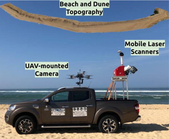
2.2. Mobile Laser Scanning and Unmanned Aircraft System

The terrestrial MLS was a SITECO Road-Scanner3 [32], equipped with three scanners (two Faro Focus S 70, one Faro Focus S 150, [33]) and mounted on an AWD car (Figure 2). Laser scanners measure points up to 150 m away from the car. Points are scanned within a 300° window at an angular resolution of 0.009°. The scan acquisition frequency was set to 60 Hz. At this frequency, accounting for the scanners’ orientation and car speed of 3.5 m·s⁻¹ (or 12.6 km·h⁻¹), the system was able to collect on the order of 60 million points per 100 m. The MLS georeferencing was ensured by an inertial navigation system including GNSS receiver (LANDINS INS, iXblue, Saint-Germain-en-Laye, France) and a GNSS antenna (Zephyr, Trimble, Sunnyvale, CA, USA). Permanent GNSS signal reception during the acquisition allowed the delivery of an accurate trajectory—time, position, attitude estimates—for the MLS, featuring high-quality GNSS parameters and a predicted accuracy below 2 cm during the entire survey. Additionally, according to manufacturer, the scanners’ accuracy at 25 m is of 0.35 cm.

The ground vehicle loaded with the MLS also carried an optical target on its roof, facing upwards (Figure 2b). The target is a slightly modified version from that in reference [24] and enables KGCP photogrammetric measurements in the aerial images. These measurements are related to the high-accuracy MLS trajectory through precisely measured geometric relations in the installation of the target.

The UAS used in the missions (Figure 2a) was provided by Octocam-maps (Valldoreix, Catalonia, Spain). It was a multi-copter based on a Super Skyjib X8 airframe (Aeronavics, Raglan, New Zealand) and a Pixhawk 2.1 autopilot, featuring a total MTOW of 11 kg and 30 min of flight time. A ground control station PC and a safety pilot with direct line-of-sight to the drone were carried in the ground vehicle. The remote sensing payloads consisted on an optical camera Lumix GH4 (Panasonic, Kadoma, Osaka, Japan) with a fixed 14 mm camera constant, installed on a gyro-stabilized mount and delivering 16 Mpx images. The geo-referencing payload consisted of an Argonaut system [34], an integrated single-frequency L1 GNSS receiver with image time-tagging and data storage capabilities.

2.3. Ground Control Points and GNSS Processing

Optical targets were deployed and surveyed in the study area (Figure 2b). Similar to Salach et al. [26], targets were arranged in six rows of three targets per row. For each row, two targets stayed on each side of the driving path and the third was placed on the dune top. In the photogrammetric process, these Ground Control Points (GCPs) were used as control points, except in the case where KGCPs were used. Then, four GCPs at the extremity of the surveyed corridor were control points and the remaining 14 GCPs were used as check points. Additionally, a multi-constellation dual-frequency GNSS base station (Trimble Zephyr) was collocated on the northern side of the survey area (Figure 3b). The position of the GNSS base station was computed in multi-base differential GNSS supported by three stations of the French Résaux GNSS Permanent (RGP), all within a 50 km distance to the north, east and south of the Bay of Arcachon.

All GNSS data collected during the missions—encompassing UAS, MLS and GCPs—were post-processed using the same deployed GNSS base station. The GCPs were surveyed using a GNSS receiver attached to a pole. The MLS time-position-attitude trajectory was obtained with both Grafnav 8.0 (Novatel, Calgary, AB, Canada) and DELPH INS (iXBlue, Saint-Germain-en-Laye, France), while the drone time-position trajectory was obtained with Grafnav 8.0. We note a difference from MLS and GCPs, where single-frequency differential processing was carried out to obtain the UAS trajectory using precise orbits and clock from the International GNSS Service (IGS). Given the proximity of the base station, it was possible to achieve a fixed-ambiguity solution with an estimated precision below five centimeters.

2.4. Geodata Acquisition and Processing

2.4.1. Mission Profiles

The survey consisted of four passes along the same 1.5-km alongshore extension, at the southern extremity of the Cap Ferret sandspit. During each pass, MLS and UAS data were collected simultaneously, at speeds ranging from 12 km·h⁻¹ to 22 km·h⁻¹ and at a constant flying height of 70 m above ground (beach) level. By doing so, the upper beach and foredune were surveyed with an average swath width of 74 m (Figure 3).

2.4.2. MLS Data Processing

Table 1. Number of raw and cleaned ground points for individual passes with associated survey speed and direction; last two columns are the mean and standard deviation of the differences between individual DEM for each pass and the reference DEM.

Cloud Id	Pass Direction	Car Speed	# of Points	# of (Cleaned) Ground pts	Bias (cm)	Std. (cm)
P1	Southward	< 3.5 m·s−1	90,124,979	87,391,199	−0.5	1.6
P2	Northward	< 3.5 m·s−1	102,224,369	100,803,317	0.1	1.5
P3	Southward	< 6 m·s−1	47,856,951	47,324,567	0.3	1.5
P4	Northward	< 5 m·s−1	60,913,147	59,924,932	0.1	1.4

summarizes the achieved MLS point cloud density according to the vehicle speed. Overall, more than 300 million points were collected. Raw point clouds from individual passes were cleaned from spurious points. Each point cloud was divided into 20 cm voxels and points within floating and isolated voxels were removed. The remaining 295,444,015 points were grouped into a single cloud, which was used to construct a reference Digital Elevation Model (DEM). This model was created with SAGA-GIS [35] following Donker et al. [20], and it was built as a regular grid with 1 m × 1 m cells where the elevation of each cell corresponds to the mean elevation of all points within the cell’s horizontal boundaries. Minimum and maximum cell heights in the reference model are −0.3 m and 19.7 m respectively, relative to the France national datum (NGF). This yields an average elevation of 4.99 m over a total surface of 87,495 m² (Figure 4a,b). The covered area includes both flat and steep zones, with maximum slope reaching 47°. Steep zones being found in the foredune and the thinner slip face of a beach ridge at the southern end of the surveyed area. These slopes are well distinguished from the flatter upper beach portion. The distinction threshold has been set to 10° (Figure 4e); this value corresponds to a break value of the slope histogram.

To assess the robustness of the acquisition and the produced reference elevation model, DEMs were created also for all four individual passes. Individual DEMs were built in a similar fashion as the above described reference DEM. For convenience, this was done with CloudCompare [36] which includes tools to ensure all grids were horizontally aligned. Indeed, for a single point cloud, sub-cell horizontal shifts of the DEM grid modify the mean height of the DEM by up to few centimeters. The last two columns of Table 1 present the differences of the aligned four DEMs with the reference elevation model. Mean differences of few millimeters and standard deviations in the order of 1.5 cm attest of the robustness of the LiDAR acquisition. In the next Section 3, the comparison of reference elevation model, directly with the individual point clouds further confirms the coherence between the data collected during the different passes.

However, the elevation of the reference DEM was, on average, 11.9 cm lower than that of the twelve GCPs measured on the upper beach. This vertical instrumental offset between the MLS trajectory and the GCPs was a posteriori corrected by shifting up of the MLS trajectory to ensure consistency between MLS, UAS and GCP products when facing the combined air-ground ISO.

2.4.3. UAS Data Processing

The UAS optical camera was configured to acquire images at a fixed frequency of 0.5 Hz. At this frequency, corresponding passes P1 and P2 (see Table 1) delivered an average number of 230 images and 88% of forward overlap, while P3 and P4 delivered around 145 images and 80% of forward overlap. At the flying height of 70 m, the obtained Ground Sampling Distance (GSD) for all passes was 1.8 cm per pixel. Note that due to the height difference between the beach and the dune, the GSD on the top of the dune was slightly better.

For conciseness, we selected pass P1 to generate the photogrammetric reconstruction results for one-pass corridor mapping. This pass was selected due to the particular, higher quality of the acquired drone geodata (GNSS ambiguity fixing, image blurring, etc.). Additionally, we note that the interest of mapKITE is to exploit the potential of one-pass corridor mapping as the optimal modality in terms of productivity despite its inherently challenging conditions due to the absence of side overlap. In particular, P1 includes 231 images with the aforementioned image overlap and GSD.

From the images in the selected pass, GCP image measurements for the eighteen targets were manually performed, as well as automated KGCP measurement to deliver photogrammetric coordinates of the optical target in the MLS vehicle (a total of 231 measurements). Then, commercial photogrammetric software (Photoscan Professional, Agisoft, St. Petersburg, Russia) was used to deliver photogrammetric matching measurements for a total of 16,738 tie points.

Finally, similarly to the workflow presented by Molina et. al [24], Integrated Sensor Orientation (ISO) was performed to estimate exterior and interior orientation parameters of the UAS images as well as the ground coordinates of the tie points. Different configurations of GCPs were used to generate two different sparse point clouds. Firstly, to represent a pure UAS-based photogrammetric approach, ISO with GNSS position-only aerial control, tie point photogrammetric measurements and the full set of 18 GCPs was performed (hereafter referred to as ISO_18GCPs). Secondly, to represent a typical mapKITE corridor, ISO with four GCPs only (two at each end of the corridor) but including the full set of 231 KGCP measurements, i.e., one per image, was also carried out (hereafter referred to as ISO_4GCPs+KGCPs). Few facts are noteworthy. First, establishing two GCPs at each corridor end is feasible operationally speaking (take-off and landing spots) as at least one can be even materialized easily with static KGCPs—when the ground vehicle remains static. Secondly, we note that self-calibration is performed to adjust interior orientation parameters during the mission. Both ISO approaches were implemented with GeoNumerics’ GENA software, a generic least-squares adjustment numerical core [37].

3. Results

In this section, we present the results obtained by the aforementioned different surveying techniques by means of statistical analysis of the differences obtained by comparing individual point clouds with the reference DEM derived from the MLS and introduced in Section 2.4.2. Results are summarized in

Table 2. Comparison of the reference surface with (row 1 to row 4) randomly-resampled MLS point clouds, (row 5 and row 6) UAS point clouds obtained with different GCP and KGCP configurations.

Cloud Id	All Points		Flat Areas		Steep Areas
	Bias (cm)	Std. (cm)	Bias (cm)	Std. (cm)	Bias (cm)	Std. (cm)
P1_resampled	0.4	9.9	−0.2	5.2	1.9	16.3
P2_resampled	1.0	8.7	0.7	2.7	1.9	15.7
P3_resampled	1.1	9.3	0.7	2.7	2.0	16.7
P4_resampled	1.0	8.8	0.7	2.4	1.9	16.2
ISO_18GCPs	1.3	13.7	−1.3	9.3	5.2	17.7
ISO_4GCPs+KGCPs	−2.0	14.4	−5.7	9.5	3.7	18.2

and further explained in each of the following sub-sections, the goal of this accuracy assessment being the demonstration that minimal GCP configuration in corridor mapping together with KGCPs delivers similar results as the configuration with all GCPs.

3.1. MLS Point Clouds

Point clouds from individual passes were first compared to the reference DEM. For the comparison, individual clouds were randomly resampled with LASTools [38], defining a minimal spatial spacing of 3 m between points. Resampling decreased the number of compared points to approximately 10,000 per pass. For each point of the resampled point clouds, the vertical distance to the reference DEM was then computed. First four rows of Table 2 summarize the comparison outcomes. Overall, results for the four passes are similar. The average difference with the reference elevation is in the order of a centimeter and the standard deviation between data sets is contained below 10 cm. Differentiating points within flat beach, with slopes below 10° as in Figure 4e, from those located in the steeper foredune, reveals increased differences in steeper areas, with bias on the order of 2 cm and standard deviation around 16 cm.

3.2. Photogrammetric Point Clouds

The comparison of photogrammetric point clouds with the reference DEM was done in similar fashion as for individual-pass resampled MLS point clouds. Both ISO approaches yield 7422 points, which are further compared to the reference are their differences summarized in Table 2. Differences for ISO point clouds are larger than for their MLS counterpart. On average, differences remain within ±2 cm for both ISO point clouds and, in terms of variance, the average of both ISO standard deviations is of 14.1 cm against 9.2 cm for the average of the standard deviation of the four MLS point clouds. Differentiating flat and steep areas further reveals that the distribution of differences is not homogeneous. Larger discrepancies between the performance of ISO and MLS point clouds occur within flat areas, where the root mean square difference ($D_{rms}$) is of 11.1 cm in the case of ISO_4GCPs+KGCPs, against 3.3 cm in average for resampled MLS point clouds. In steep areas, performances are more similar, with $D_{rms}$ of 18.6 cm and 16.3 cm for respectively ISO_4GCPs+KGCPs and MLS point clouds. Finally, the overall performance of both ISO approaches are analogous, with $D_{rms}$ values of 13.8 cm and 14.5 cm for ISO_18GCPs and ISO_4GCPs+KGCPs respectively.

Check point accuracy analysis, i.e., the accuracy estimation of the ground coordinates for fourteen GCPs (out of 18, those not used in the ISO_4GCPs+KGCPs), provides additional insights into the method performance. For these points, RMS errors of 2.6 cm, 3.6 cm and 13.2 cm were achieved in easting, northing and height, respectively. Although the check point sample is less exhaustive than the MLS one, these statistical results are totally comparable to those in the last row of Table 2.

3.3. Photogrammetric DEMs

To provide a qualitative description of each methods in terms of 3D morphology, the sparse photogrammetric point clouds were triangulated with a Delaunay triangulation. Figure 4c presents the 1 m × 1 m DEM interpolated from the triangulated ISO_4GCPs+KGCPs point cloud, and Figure 5 presents the spatial distribution of differences between photogrammetric DEMs and the reference DEM derived from the MLS. Darker colors for ISO_4GCPs+KGCPs are coherent with the slightly larger $D_{rms}$ values. However, the distributions are very similar for both ISO approaches. In both cases, larger differences are present along the foredune slope, with an overall pattern of a higher foredune bordered by a lower beach. At the scale of the common ISO-MLS cross-shore profile, ranging about 8 m vertically, differences are minimal (Figure 5c). For convenience, on each of the profile plots, the two ISO profiles were also plotted with a vertical offset. This reveals notable similarities in the results from both ISO approaches and excellent matches with the reference DEM. Also, sparse ISO point clouds appear to be sufficient to capture the morphological features across each of the profiles, as well, UAS-based DEMs extend beyond the foredune, up to areas out of reach for the MLS system.

4. Discussion

4.1. Experiment Originality

The selected point clouds and DEMs presented above, have been produced based on an experiment involving a hybrid UAS and MLS system. The experiment was designed to investigate how the cost-accuracy ratio of UAS photogrammetry could be improved for topographic applications along beach corridors; it was motivated by the interest that a flexible and efficient corridor mapping solution would represent for monitoring long coastal stretches before and after storms.

Presently, the accuracy of UAS-based photogrammetry remains largely dependant on both the acquisition of GCPs and on robust flight geometry (

Table 3. Comparison of photogrammetric performance with selected coastal topography applications, in terms of root mean square errors ($E_{rms}$), as a function of the number of GCPs per surveyed area/extent, of above ground flight level (AGL), of Ground Sampling Distance (GSD) and of image overlap, in one or two horizontal dimensions.

Ref.	${\mathit{E}}_{\mathit{rms}}$ (cm)	# of GCPs	Extent (m)	AGL (m)	GSD (cm)	Image Overlap
Mancini et al. [39]	22.0	18	2.7 ha	40	0.6	2D
Gonçalves et al. [40]	4.6	12	800 × 500	131	4.5	2D
Long et al. [41]	16	56	400 ha	150	4.6	2D
Turner et al. [13]	7.3	0	3500 × -	100	3.4	2D
Sturdivant et al. [11]	3.6	18	500 × 300	35	2.5	2D
Elsner et al. [27]	8	49	450 × 150	70	1.7	2D
Ruessink et al. [43]	6.7; 10.7	33; 39	800 × 500	-	-	2D
Gonçalves et al. [46]	12	10	700 × 100	80 and 100	4.7	2D
Laporte-Fauret et al. [44]	5	5	1000 × 350	70	1.78	2D
ISO_18GCPs	13.8	18	1500 × 70	70	1.8	1D
ISO_4GCPs+KGCPs	14.5	4	1500 × 70	70	1.8	1D

; [11,16,39,40,41,42,43,44]). In terms of field effort, the first issue translates into time-consuming georeferencing of stable ground points [44] and/or ad-hoc deployment and surveying of optical targets. The second issue requires that images overlap both along and across flight direction. This can be achieved in the case of parallel flight lanes, which at least doubles survey time.

Given these conditions, the experiment design is original, both because of the single-pass flight geometry and because of the reduced number of GCPs, and the MLS data, which is an established technology to survey beach foredunes [20], could be used as ground truth to validate this innovative survey strategy.

4.2. Hybrid UAS-MLS Performance

For validation purposes, a reference DEM was generated by merging MLS point clouds collected during four passes (P1 to P4 in Table 1). This reference was then compared to DEMs from individual passes and randomly resampled individual point clouds, attesting that the survey robustness was in line with MLS standards in sandy beach application [20]. The reference DEM then served to assess the quality of two photogrammetric point clouds generated by integrated sensor orientation, first with all available GCPs (eighteen) and then with only 4 GCPs and the available KGCPs (231 in total). Both photogrammetically-generated point clouds delivered similar performances, the root mean square of elevation differences with the reference DEM ($D_{rms}$) being of 13.8 cm for ISO_18GCPs and of 14.5 cm for ISO_4GCPs+KGCPs.

Table 3 puts those numbers into perspective with the $E_{rms}$ values claimed in published applications of photogrammetric topography in sandy coastal settings. In addition to Li et al. [45], who presented a comparison of the performance for different types of cameras and UAS platforms, the range of values in Table 3 recalls that the quality of photogrammetric products is also sensitive to a wide range of instrumental and environmental parameters. For instance, Gonçalves et al. [40] and Long et al. [41] acquired and processed data in a very similar fashion, but still achieved performances which are quite different. Moreover, there is no unique way of comparing point clouds. For instance, Turner et al. [13] compared the ground elevation, measured with a GNSS receiver mounted on an all-terrain vehicle (ATV), against the average elevation of their high-density photogrammetric point cloud within a horizontal square meter centered on the ATV. Similarly, authors using a greater number of GCPs, surveyed with a pole-mounted GNSS receiver, mostly compared GCPs’ elevation with the elevation interpolated onto the photogrammetrically-derived DEMs [11,40,41,44]. When both laser (terrestrial or airborne) and photogrammetric data are available, a classic approach is to compare the respectively generated DEMs [27,39,46]. Such comparison implies a densification of the photogrammetric point cloud and, as pointed out by Elsner et al. [27], may smooth differences compared to the comparison of raw point clouds. Here, the choice was made to quantify the deviation of sparse photogrammetric measurements, from a denoised and a priori more accurate surface.

Considering these possible technical and methodological differences, $D_{rms}$ values achieved in this study are very much in line with the expected performance of photogrammetric point clouds. In particular, the performance achieved in this study are better or very close to that of Mancini et al. [39], Elsner et al. [27] and Gonçalves et al. [46] who also compared their photogrammetric point clouds with terrestrial or airborne laser scanner measurements. To be noted also is that $E_{rms}$ achieved by Laporte-Fauret et al. [44] with 4 GCPs increases up to 0.5 m to 1.12 m (depending on the camera quality) as they compared their photogrammetric DEMs with 5 across-foredune GNSS profiles.

Likewise, some authors claim performances that are slightly better than those presented herein. For instance, Sturdivant et al. [11] achieved an umatched $E_{rms}$ of 3.6 cm, with the lowest above ground flight level (AGL) which also means a lower coverage-to-flight time ratio. Also, increasing the number of GCPs has limits in approving the measurement accuracy. See for instance the relative accuracy in Laporte-Fauret et al. [44] and in Ruessink et al. [43] who used a greater number of GCPs. To be noted as well is that the accuracy in Laporte-Fauret et al. [44] is capped at 5 cm with either 5 or 10 GCPs, similar to results of Tonkin et al. [42] with either 4 or 101 GCPs. In this respect, mapKITE appears to provide just the required control to match the achievable accuracy, taking into account other instrumental and environmental constraints.

Another important point is that these previous studies rely on more complex flight trajectories, allowing for image overlap in the 2D horizontal plane. Even with differential GNSS processing techniques, it is expected that 2D image overlap should help reduce errors as in the case of Turner et al. [13]. In the present case, little constraint perpendicularly to the flight direction may have added to the errors and could explain why, even with 18 GCPs, $D_{rms}$ does not reach the lowest cited values. Indeed, the opposed mean differences on the beach and along the steeper foredune seems to come from a horizontal mismatch or a tilt in the photogrammetric point clouds. Such tilting could be due to less robust image overlaps. Still, with this minimal flight geometry and, in the case ISO_4GCPs+KGCPs, a reduced number of GCPs, observed differences remain within photogrammetric standards.

Regarding the problems that may arise when performing single linear UAS pass, results are good and encouraging. On the beach, the higher variance of the photogrammetric point clouds, compared to the MLS point clouds, contrasts with more similar performances along the foredune slope, and is compensated by extended geodata coverage. The good match between profiles extracted from the DEM produced with the sparse point cloud and those extracted from the reference DEM reveals that photogrammetric point cloud densification was unnecessary to capture the morphological features of the beaches and foredunes.

4.3. Foreseen Applications

Regarding classic GCP-based photogrammetry, mapKITE makes it possible to significantly reduce field efforts and survey duration. This becomes critical, for instance, during emergency situations, when shoreline data is needed over long corridors. Most important, the achieved vertical accuracy is appropriate for quantifying the impact of storms along open beaches similar to those of the Atlantic Coast of France, which are on the order of several meters [17]. Therefore, the mapKITE concept becomes a credible alternative for capturing the impact of storms over long portions of coast with maximum responsiveness.

For such applications, alternatives also include UAS equipped with an IMU/GNSS solution and/or with ultra-light laser scanners [13,26]. Still, compared to lightweight solutions for aerial navigation control, the high grade IMU/GNSS system embarked on the present terrestrial-aerial tandem limits performance degradation as a function of base-to-rover distance. This latter aspect becomes significant when considering surveys of several tens of kilometers.

5. Conclusions

Different mapping methods were used for surveying a beach prone to erosion and backed by steep foredunes. The simultaneous acquisition of mobile laser scanning data and UAS photos has enabled the cross-validation of different topographic products. Along a narrow and linear corridor, the laser system and the UAS were operated according to the mapKITE concept. In this configuration, UAS photogrammetry can benefit from the use of KGCPs. Benefits include: (1) a reduced number of GCPs (only support GCPs at the ends of the corridor) and (2) the possibility to carry on single pass survey. This is made possible as, through those KGCPs, the photogrammetric measurements also assimilate data from a high-grade IMU/GNSS system. After a first series of conclusive tests for road mapping [24], this approach was found to perform equally well in sandy coastal settings, with a vertical accuracy of at least within 15 cm RMS for topographic measurements derived from UAS photogrammetry. Furthermore, the assimilation of high-grade IMU/GNSS data ensures this accuracy can be matched over the longest extension. Along with UAS equipped with RTK solutions, mapKITE proves to be an alternative for the topographic survey of linear stretch of coast in emergency situations and at minimal logistic cost.

References

1. Elko, N.A.; Feddersen, F.; Foster, D.; Hapke, C.J.; McNinch, J.E.; Mulligan, R.P.; Tuba Özkan Haller, H.; Plant, N.G.; Raubenheimer, B. The future of nearshore processes research. Shore Beach 2015, 83, 13–38. [Google Scholar]
2. IPCC. Coastal Systems and Low-Lying Areas. In Climate Change 2014—Impacts, Adaptation and Vulnerability: Part A: Global and Sectoral Aspects: Working Group II Contribution to the IPCC Fifth Assessment Report; Cambridge University Press: Cambridge, UK, 2014; Volume 1, pp. 361–410. [Google Scholar] [CrossRef]
3. Masselink, G.; Castelle, B.; Scott, T.; Dodet, G.; Suanez, S.; Jackson, D.; Floc’h, F. Extreme wave activity during 2013/2014 winter and morphological impacts along the Atlantic coast of Europe. Geophys. Res. Lett. 2016, 43, 2135–2143. [Google Scholar] [CrossRef]
4. Splinter, K.D.; Harley, M.D.; Turner, I.L. Remote Sensing Is Changing Our View of the Coast: Insights from 40 Years of Monitoring at Narrabeen-Collaroy, Australia. Remote Sens. 2018, 10, 1744. [Google Scholar] [CrossRef]
5. Almeida, L.; Almar, R.; Bergsma, E.; Berthier, E.; Baptista, P.; Garel, E.; Dada, O.; Alves, B. Deriving High Spatial-Resolution Coastal Topography From Sub-meter Satellite Stereo Imagery. Remote Sens. 2019, 11, 590. [Google Scholar] [CrossRef]
6. Ruessink, G.; Schwarz, C.S.; Price, T.D.; Donker, J.J.A. A Multi-Year Data Set of Beach-Foredune Topography and Environmental Forcing Conditions at Egmond aan Zee, The Netherlands. Data 2019, 4, 73. [Google Scholar] [CrossRef]
7. European Commission. Report on the Blue Growth StrategyTowards More Sustainable Growth And Jobs in the Blue Economy; European Commission: Brussels, Belgium, 2017. [Google Scholar]
8. Turner, I.L.; Harley, M.D.; Short, A.D.; Simmons, J.A.; Bracs, M.A.; Phillips, M.S.; Splinter, K.D. A multi-decade dataset of monthly beach profile surveys and inshore wave forcing at Narrabeen, Australia. Sci. Data 2016, 3, 160024. [Google Scholar] [CrossRef] [PubMed]
9. Le Mauff, B.; Juigner, M.; Ba, A.; Robin, M.; Launeau, P.; Fattal, P. Coastal monitoring solutions of the geomorphological response of beach-dune systems using multi-temporal LiDAR datasets (Vendée coast, France). Geomorphology 2018, 304, 121–140. [Google Scholar] [CrossRef]
10. Colomina, I.; Molina, P. Unmanned aerial systems for photogrammetry and remote sensing: A review. J. Photogramm. Remote Sens. 2014, 92, 79–97. [Google Scholar] [CrossRef] [Green Version]
11. Sturdivant, E.J.; Lentz, E.E.; Thieler, E.R.; Farris, A.S.; Weber, K.M.; Remsen, D.P.; Miner, S.; Henderson, R.E. UAS-SfM for Coastal Research: Geomorphic Feature Extraction and Land Cover Classification from High-Resolution Elevation and Optical Imagery. Remote Sens. 2017, 9, 1020. [Google Scholar] [CrossRef]
12. Eltner, A.; Kaiser, A.; Castillo, C.; Rock, G.; Neugirg, F.; Abellán, A. Image-based surface reconstruction in geomorphometry merits, limits and developments. Earth Surf. Dyn. 2016, 4, 359–389. [Google Scholar] [CrossRef]
13. Turner, I.L.; Harley, M.D.; Drummond, C.D. UAVs for coastal surveying. Coast. Eng. 2016, 114, 19–24. [Google Scholar] [CrossRef]
14. Rehak, M. Integrated Sensor Orientation on Micro Aerial Vehicles; EPFL: Lausanne, Switzerland, 2017; p. 226. [Google Scholar]
15. Tournadre, V.; Pierrot-Deseilligny, M.; Faure, P.H. UAV linear photogrammetry. Int. Arch. Photogramm. Remote Sens. Spat. Inf. Sci. 2015, XL-3/W3, 327–333. [Google Scholar] [CrossRef]
16. Jaud, M.; Passot, S.; Allemand, P.; Le Dantec, N.; Grandjean, P.; Delacourt, C. Suggestions to Limit Geometric Distortions in the Reconstruction of Linear Coastal Landforms by SfM Photogrammetry with PhotoScan® and MicMac® for UAV Surveys with Restricted GCPs Pattern. Drones 2019, 3, 2. [Google Scholar] [CrossRef]
17. Castelle, B.; Marieu, V.; Bujan, S.; Splinter, K.D.; Robinet, A.; Sénéchal, N.; Ferreira, S. Impact of the winter 2013–2014 series of severe Western Europe storms on a double-barred sandy coast: Beach and dune erosion and megacusp embayments. Geomorphology 2015, 238, 135–148. [Google Scholar] [CrossRef]
18. Barber, D.M.; Mills, J.P. Vehicle Based Waveform Laser Scanning in a Coastal Environment. In Proceedings of the 5th International Symposium on Mobile Mapping Technology, Padua, Italy, 29–31 May 2007; p. 6. [Google Scholar]
19. Bitenc, M.; Lindenbergh, R.; Khoshelham, K.; Van Waarden, A.P. Evaluation of a LIDAR Land-Based Mobile Mapping System for Monitoring Sandy Coasts. Remote Sens. 2011, 3, 1472–1491. [Google Scholar] [CrossRef] [Green Version]
20. Donker, J.; van Maarseveen, M.; Ruessink, G. Spatio-Temporal Variations in Foredune Dynamics Determined with Mobile Laser Scanning. J. Mar. Sci. Eng. 2018, 6, 126. [Google Scholar] [CrossRef]
21. Lim, S.; Thatcher, C.A.; Brock, J.C.; Kimbrow, D.R.; Danielson, J.J.; Reynolds, B.J. Accuracy assessment of a mobile terrestrial lidar survey at Padre Island National Seashore. Int. J. Remote Sens. 2013, 34, 6355–6366. [Google Scholar] [CrossRef]
22. Molina, P.; Blázquez, M.; Sastre, J. mapKITE: A New Paradigm for Simultaneous Aerial and Terrestrial Geodata Acquisition and Mapping. In Proceedings of the International Archives of the Photogrammetry, Remote Sensing and Spatial Information Sciences, Prague, Czech Republic, 12–19 July 2016. [Google Scholar]
23. Molina, P.; Blázquez, M.; Sastre, J.; Colomina, I. Precision Analysis of Point-And Photogrammetric Measurements for Corridor Mapping: Preliminary Results. Int. Arch. Photogramm. Remote Sens. Spat. Inf. Sci. 2016, 85–90. [Google Scholar] [CrossRef]
24. Molina, P.; Blázquez, M.; Cucci, D.A.; Colomina, I. First Results of a Tandem Terrestrial-Unmanned Aerial mapKITE System with Kinematic Ground Control Points for Corridor Mapping. Remote Sens. 2017, 9, 60. [Google Scholar] [CrossRef]
25. Baltsavias, E.P. A comparison between photogrammetry and laser scanning. ISPRS J. Photogramm. Remote Sens. 1999, 54, 83–94. [Google Scholar] [CrossRef]
26. Salach, A.; Bakuła, K.; Pilarska, M.; Ostrowski, W.; Górski, K.; Kurczyński, Z. Accuracy Assessment of Point Clouds from LiDAR and Dense Image Matching Acquired Using the UAV Platform for DTM Creation. ISPRS Int. J. Geo.-Inf. 2018, 7, 342. [Google Scholar] [CrossRef]
27. Elsner, P.; Dornbusch, U.; Thomas, I.; Amos, D.; Bovington, J.; Horn, D. Coincident beach surveys using UAS, vehicle mounted and airborne laser scanner: Point cloud inter-comparison and effects of surface type heterogeneity on elevation accuracies. Remote Sens. Environ. 2018, 208, 15–26. [Google Scholar] [CrossRef]
28. European Commission. NEPTUNE Blue Growth Accelerator. 2018. Available online: www.neptune-project.eu (accessed on 6 March 2019).
29. Castelle, B.; Guillot, B.; Marieu, V.; Chaumillon, E.; Hanquiez, V.; Bujan, S.; Poppeschi, C. Spatial and temporal patterns of shoreline change of a 280-km high-energy disrupted sandy coast from 1950 to 2014: SW France. Estuar. Coast. Shelf Sci. 2018, 200, 212–223. [Google Scholar] [CrossRef]
30. Nahon, A.; Idier, D.; Sénéchal, N.; Féniès, H.; Mallet, C.; Mugica, J. Imprints of wave climate and mean sea level variations in the dynamics of a coastal spit over the last 250 years: Cap Ferret, SW France. Earth Surf. Process. Landf. 2019. [Google Scholar] [CrossRef]
31. Nahon, A. Ongoing Morphological Evolution of a Holocene Coastal Barrier Spit: The Cap Ferret, at the Entrance of the Bay of Arcachon. Ph.D. Thesis, Université de Bordeaux, Bordeaux, France, 2018. [Google Scholar]
32. SitecoInformatica. Brochure Road-Scanner 3; Technical Report; SitecoInformatica: Bologna, Italy, 2016. [Google Scholar]
33. FARO. FARO Laser Scanner Focus M&S Tech Sheet; FARO: Lake Mary, FL, USA, 2019. [Google Scholar]
34. Rokubun. Brochure Argonaut; Technical Report; Rokubun: Barcelona, Spain.
35. Conrad, O.; Bechtel, B.; Bock, M.; Dietrich, H.; Fischer, E.; Gerlitz, L.; Wehberg, J.; Wichmann, V.; Böhner, J. System for Automated Geoscientific Analyses (SAGA) v. 2.1.4. Geosci. Model Dev. 2015, 8, 1991–2007. [Google Scholar] [CrossRef] [Green Version]
36. CloudCompare. GPL Software, Version 2.10. 2019. Available online: www.cloudcompare.org (accessed on 18 March 2019).
37. Colomina, I.; Blázquez, M.; Navarro, J.; Sastre, J. The need and keys for a new generation network adjustment software. Int. Arch. Photogramm. Remote Sens. Spat. Inf. Sci. 2012, XXXIX-B1, 303–308. [Google Scholar] [CrossRef]
38. Isenburg, M. LAStools; rapidlasso GmbH: Gilching, Germany, 2012. [Google Scholar]
39. Mancini, F.; Dubbini, M.; Gattelli, M.; Stecchi, F.; Fabbri, S.; Gabbianelli, G. Using Unmanned Aerial Vehicles (UAV) for High-Resolution Reconstruction of Topography: The Structure from Motion Approach on Coastal Environments. Remote Sens. 2013, 5, 6880–6898. [Google Scholar] [CrossRef] [Green Version]
40. Gonçalves, J.; Henriques, R. UAV photogrammetry for topographic monitoring of coastal areas. J. Photogramm. Remote Sens. 2015, 104, 101–111. [Google Scholar] [CrossRef]
41. Long, N.; Millescamps, B.; Guillot, B.; Pouget, F.; Bertin, X. Monitoring the Topography of a Dynamic Tidal Inlet Using UAV Imagery. Remote Sens. 2016, 8, 387. [Google Scholar] [CrossRef]
42. Tonkin, T.; Midgley, N. Ground-Control Networks for Image Based Surface Reconstruction: An Investigation of Optimum Survey Designs Using UAV Derived Imagery and Structure-from-Motion Photogrammetry. Remote Sens. 2016, 8, 786. [Google Scholar] [CrossRef]
43. Ruessink, B.G.; Arens, S.M.; Kuipers, M.; Donker, J.J.A. Coastal dune dynamics in response to excavated foredune notches. Aeolian Res. 2018, 31, 3–17. [Google Scholar] [CrossRef]
44. Laporte-Fauret, Q.; Marieu, V.; Castelle, B.; Michalet, R.; Bujan, S.; Rosebery, D. Low-Cost UAV for High-Resolution and Large-Scale Coastal Dune Change Monitoring Using Photogrammetry. J. Mar. Sci. Eng. 2019, 7, 63. [Google Scholar] [CrossRef]
45. Li, H.; Chen, L.; Wang, Z.; Yu, Z. Mapping of River Terraces with Low-Cost UAS Based Structure-from-Motion Photogrammetry in a Complex Terrain Setting. Remote Sens. 2019, 11, 464. [Google Scholar] [CrossRef]
46. Gonçalves, G.R.; Pérez, J.A.; Duarte, J. Accuracy and effectiveness of low cost UASs and open source photogrammetric software for foredunes mapping. Int. J. Remote Sens. 2018, 39, 5059–5077. [Google Scholar] [CrossRef]
Figure 1. Satellite images of the study area on 26 September 2018. (a) Landsat image of the Cap Ferret barrier-spit and of the Bay of Arcachon. (b) Sentinel image of the surveyed beach and intertidal bars at the spit’s southern extremity.
Remotesensing 11 01352 g001
Figure 2. MLS and UAS systems. (a) MLS system mounted on a 4WD car and UAS during its take off (Photo courtesy of Denis Lherm, Sud Ouest). (b) UAS view of the MLS roof-mounted optical target and a GCP (A4 size checkerboard).
Remotesensing 11 01352 g002
Figure 3. On site survey. (a) UAS orthophoto on top of Sentinel satellite imagery, with the GNSS base station (red star), the ground control points (black/white circles) and the car trajectory (black line). (b) The MLS heading southward with the dune cliff in the background.
Remotesensing 11 01352 g003
Figure 4. Digital Elevation Models (DEMs). (a,b) Regular grid elevation model derived from MLS point cloud. (c) Same as (b) for the elevation model obtained after triangulating sparse point cloud computed by photogrammetry (ISO_4GCPs+KGCPs). Symbols on (a,c) are the same as on Figure 3a; on (b,c) isocontours are 1-m spaced with +6 m NGF shown in red. (d) Same DEM as (c), but draped with the orthophoto generated with the UAS images. (e) Same DEM as (c), with the red and blue shades corresponding respectively to the steep and flat areas in the MLS-derived DEM.
Remotesensing 11 01352 g004
Figure 5. 3D topographic surface comparison. (a,b) Differential surfaces of the ISO_18GCPs (a) and ISO_4GCPs+KGCPs (b) elevation models minus MLS elevation model. (c) Profiles extracted along three cross-shore sections, from the MLS reference DEM (black curves), from the two photogrammetric DEMs and from the vertically shifted photogrammetric DEMs (colored curves).
Remotesensing 11 01352 g005