Detecting Power Lines in UAV Images with Convolutional Features and Structured Constraints

Abstract

Power line detection plays an important role in an automated UAV-based electricity inspection system, which is crucial for real-time motion planning and navigation along power lines. Previous methods which adopt traditional filters and gradients may fail to capture complete power lines due to noisy backgrounds. To overcome this, we develop an accurate power line detection method using convolutional and structured features. Specifically, we first build a convolutional neural network to obtain hierarchical responses from each layer. Simultaneously, the rich feature maps are integrated to produce a fusion output, then we extract the structured information including length, width, orientation and area from the coarsest feature map. Finally, we combine the fusion output with structured information to get a result with clear background. The proposed method fully exploits multiscale and structured prior information to conduct both accurate and efficient detection. In addition, we release two power line datasets due to the scarcity in the public domain. The method is evaluated on the well-annotated power line datasets and achieves competitive performance compared with state-of-the-art methods.

1. Introduction

With the rapid development of UAV techniques in electricity inspection, a growing number of power line detection methods have been developed in recent years. However, the existing methods still remain problematic in practical applications in terms of accuracy and efficiency. This paper addresses the challenge by presenting a new framework for power line detection.

1.1. Motivation and Objective

Power lines are vital components to modern industry and social urban life, so regular inspection is necessary to make sure power lines are in good condition or to help us find where to maintain them. In general, inspection of high-voltage power lines may be very dangerous and time-consuming if performed by even skilled linemen. The automated UAV-based power line inspection system developed for this task can save a lot of money, time and avoid dangerous accidents. Particularly, power line detection is one of the most important modules among the system. Accurate identification and localization of power lines can be useful for its autonomous navigation. As a result, accurate and efficient power line detection methods are very desirable in this domain.

Generally, power lines in the images taken by UAVs are cluttered with noisy background. The lines are usually surrounded by leaves, branches and tiles, some parts are even completely covered, which poses substantial challenges to traditional gradient-based methods. Most of the existing methods rely on complicated parameter settings, which makes them less stable in practical use. Besides, the characteristics of power lines differentiate the task from conventional edge detection and image segmentation in natural images. We need to consider the structures of power lines for accurate detection. The CNN-based methods can produce multiscale and hierarchical feature maps, where there are salient objects with global contours at coarse levels as well as detailed objects with accurate edge localization at fine levels. The mechanism of multiscale representations resembles the visual perception system of humans, which identifies the contour of object from high-level predictions and obtains accurate edge localization from low-level predictions. We can explore to use convolutional features and structured constraints for power line detection. However, how to extract the intrinsic structures of power lines and how to make full use of the multiscale feature maps are key problems to the task. Another problem is the lack of large public datasets with pixel-wise annotations. Previous researchers have mainly tested and evaluated their methods on several sample images or synthetic ones, which may be inappropriate for learning-based methods. To overcome this, we need to collect aerial power line images using UAVs and acquire pixel-level annotations.

1.2. Related Works

With the growing demand for automatic power line inspection, many methods have been developed over the years [1]. It is of great importance to investigate the literature on power line detection. Currently, many researchers focus on the analysis of LiDAR data for power line detection [2,3,4], which gives high-precision 3D point cloud data of surroundings. However, these kinds of methods are costly and inconvenient for practical use. Therefore, we mainly concentrate on image-based methods. Generally speaking, the existing methods for image-based power line detection can be divided into two categories, traditional gradient-based ones and learning-based ones. Here, we briefly introduce some representative approaches.

(1) Traditional gradient-based methods: Previous works mainly focus on low-level local features of gradients, brightness, textures and other prior information. These methods are specifically designed based on the assumption that power lines are straight lines or polynomial curves with the lowest intensity in image and parallelism to each other. These works first distinguish the potential pixels of power lines from background by using edge detector, such as Canny and Sobel, then Hough transformation and hand-designed filters are adopted to detect line segments followed by prior information to refine the detected results. Finally, perceptual grouping methods are exploited to link the fragments for complete line structure. Yan et al. [5] adopted Radon transform to extract line segments, followed by grouping method and Kalman filter to connect segments into entire line. On top of the task, Chen et al. [6] developed an improved version, cluster Radon transform, to detect linear feature of power line from high resolution remote sensing images. Li et al. [7] proposed to detect lines by Hough transformation, then applied K-means clustering based on parallelism to refine the results. Candamo et al. [8] fully exploited the motion information of pixels between frames and developed methods for videos, in which the feature map was computed by the combination of the edge map and the estimated motion, followed by a windowed Hough transformation to fit the lines, the parameter space of hough transformation is tracked using a line motion model. Song et al. [9] presented a sequential local-to-global power line detection method. The matched filter and first-order derivative of Gaussian were used to detect segments, then graph-cut model was adopted to group the fragments. Luo et al. [10] proposed an object-aware definition for power lines in joint RGB-NIR images to extract potential segments, followed by intensity features from NIR images to refine outputs. Zhang et al. [11,12] applied a hand-designed filter to extract power line features, then adopted epipolar constraints to refine power line segments. Although this kind of approaches have achieved great improvements in recent years, the limitations are still obvious when applied to real environment. For instance, it’s not easy to manually tune dozens of parameters to get optimal result for each image during inspection. Hence, the methods tend to produce more false positives and negatives on a whole dataset when parameters are fixed.

(2) Learning-based methods: With the explosive development of deep learning, the border of various tasks in computer vision has been pushed to a substantially higher level. In boundary detection, it can be seen from the Berkeley benchmark [13,14] that CNN-based methods [15,16,17,18] have demonstrated extraordinary performance. Since these methods share the strong ability to learn multiscale features and perceive global information, they can produce high-level representations of objects in natural images. Although the task of power line detection differs from countour detection in natural images, the desirable characteristic of multiscale fine-to-coarse responses can be used in the detection of power lines. Moreover, the end-to-end convolutional neural network can give accurate and efficient prediction without hand-designed features and threshold tuning. R. Madaan et al. [19] developed the power line detection framework using dilated convolutional networks. In the method, power line detection was treated as a semantic segmentation task. Leveraging the recent advances [20] in semantic segmentation, they designed several networks using dilated convolution with different architectures, and evaluated on both real environmental and synthetic datasets to find the optimal one. The performance boosts a lot compared with traditional methods and it is efficient on onboard platform NVIDIA Jetson TX2. However, the output is still noisy without using prior information and structures of power lines.

1.3. Contribution of The Work

In this paper, we develop an accurate and efficient framework for power line detection, which utilizes multiscale features and structured priors to produce high-level predictions. The network is built to gather different levels of line responses on the basis of VGG16 [21]. Hierarchical predictions can be obtained from different convolutional layers. The network can automatically learn how to combine different levels of information to produce satisfying fusion output. Then, the statistics of structured features, including length, width and orientation, are calculated from the last stage of conv layers for noise reduction. Finally, the standard non-maximum suppression (NMS) is adopted to refine boundaries for fair comparison. The proposed method is evaluated on the two datasets and achieves superior performance in terms of both accuracy and efficiency compared with other methods. The main contributions of the paper can be concluded as twofold:

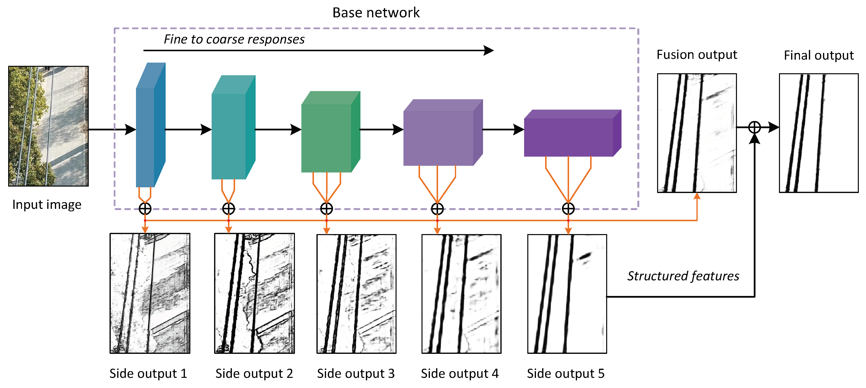
• A power line detection method is proposed by using convolutional features and structured constraints. We fully exploit the coarse-to-fine feature maps generated by the convolutional layers, which are integrated to produce a fusion output. The structured features are extracted from the coarsest feature map and then combined with fusion output to sweep out noisy segments.
• Two public datasets with pixel-level annotations are released for power line detection. We collect aerial power line images using UAVs in two different scenes and annotate the images with pixel-level precision. The datasets will be useful for developing learning-based methods in power line detection.

The remainder of this paper is organized as follows. Section 2 first analyzes network architecture, the modified loss function and the extraction of structured features. The detailed description of power line datasets is presented in Section 3. Next, experimental results are given in Section 4, and capabilities and limitations are discussed in Section 5. Finally, the conclusions are presented in Section 6.

2. Power Line Detection

2.1. Network Architecture

In this section, we give a detailed description on the network architecture of the proposed power line detection framework. In recent years, VGG16 and its variants have exhibited excellent performance in multiple computer vision tasks, such as object detection, semantic segmentation and boundary detection. The original VGG16 network is composed of three fully connected layers and thirteen convolutional layers, which are divided into five stages by four pooling layers. The convolutional layers with different strides can capture multiscale features and produce hierarchically coarse-to-fine responses, which is one of the most desirable characteristics. The fusion of multi-level information may help to perceive global feature maps of power lines with accurate localization precision. Therefore, we adopt the trimmed VGG16 architecture as the backbone of our framework which is developed in [22]. Figure 1 depicts how we make full use of the multiscale information and structured features provided by the intermediate layers of the network to accurately distinguish power lines from background. The different side outputs, produced by combining all the convolutional feature maps in each stage, contain distinguishing and scale-specific information. The fusion output is optimally generated by applying deep supervision on each side output. Integrated with structured information extracted from the fifth side output, our framework produces the accurate power lines with clear background.

The original VGG16 is specially designed for object detection and classification, which is not suitable for the task of power line detection. Therefore, we make the following modifications to adapt the network to our task: (1) The fully connected layers and the fifth pooling layer are dropped. On the one hand, the fully connected layers are specifically designed for classification tasks and have a large number of parameters. We can get the fully convolutional network like FCN [23] and greatly reduce computational cost during training and testing by the removal. On the other hand, we can observe from

Table 1. The detailed receptive field and stride size in original VGG16 net.

layer	conv1_1	conv1_2	pooling1	conv2_1	conv2_2	pooling2
rf size	3	5	6	10	14	16
stride	1	1	2	2	2	4
layer	conv3_1	conv3_2	conv3_3	pooling3	conv4_1	conv4_2
rf size	24	32	40	44	60	76
stride	4	4	4	8	8	8
layer	conv4_3	pooling4	conv5_1	conv5_2	conv5_3	pooling5
rf size	92	100	132	164	196	212
stride	8	16	16	16	16	32

that the interpolated feature map of the fifth pooling layer with stride 32 may be too coarse to be utilized. Neither detailed information nor global structure can be obtained from the feature map, so that it is regarded as un-meaningful response; (2) Each convolutional layer is connected to a layer with kernel size 1 × 1 and channel depth 21. The 1 × 1 conv layer is adopted to decrease the channels and organize feature maps. The number of channel depth has little effect on the results when it is in some range, such as tens of channels. The responses of conv layers in each stage are accumulated by an eltwise layer to produce blended feature maps. A conv layer with kernel size 1 × 1 and channel depth 1 is followed to reduce the dimension of feature maps, then a deconvolutional layer is adopted to perform bilinear interpolation, up-sampling the side output to be as large as the original input image. We can notice from the experiments in [22,24] that each individual side output contributes to the fusion result, so the overall performance will decrease if any of the side response is removed. They further show that the strategy of using all the convolutional feature maps is superior to only using the last convolutional feature map in each stage. As a result, we choose to use the former one as our strategy; (3) A class-balanced cross-entropy loss function is linked to the deconv layer in each stage. All the side-outputs are fused according to weights by a 1 × 1 conv layer, then loss is computed using the same function. The parameters of the network are determined by minimizing the sum of side-output losses and fusion loss. The structured features extracted from the fifth side output are applied to the fusion output to refine the results when network training is finished.

The convolutional layers with different reception field sizes can capture multiscale features. The shallower layers with smaller reception field size tend to capture detailed features, while the deeper layers are more sensitive to global features. The network takes full advantage of all feature maps extracted by convolutional layers and automatically learns how to combine the features to obtain superior outputs. Moreover, we benefit a lot from the structure that network training and testing can be handled in an end-to-end manner with deep supervision on different levels of side outputs.

2.2. Class-Balanced Loss Function

For the task of power line detection, the proportion of power line pixels and background pixels is seriously biased. For example, the percentage of power line pixels is less than 10% in our dataset. We need to modify the standard cross-entropy loss function to adapt to the heavily biased datasets. The class-balanced cross-entropy function proposed in [24] is used in our network. By introducing a class-balanced weight $\beta$, the imbalance between edge and non-edge pixels can be solved. The annotations of the ground truth in our two datasets are binary, 1 for power line pixels and 0 for background pixels. Thus, the problem of dealing with faint annotations in BSDS500 [25] doesn’t exist in our work. The loss function of each image in stage m is defined as:

$$\begin{array}{c}\hfill L_{side}^{(m)}(x_i;W,w^{(m)})=-\beta \sum _{i\in Y^{+}}logP(y_i=1|x_i;W,w^{(m)})\\ \hfill -\lambda (1-\beta )\sum _{i\in Y^{-}}log(1-P(y_i=0|x_i;W,w^{(m)}))\end{array}$$

(1)

in which

$$\beta =\frac{|Y^{-}|}{|Y^{+}|+|Y^{-}|}$$

(2)

$Y^{+}$ and $Y^{-}$ denote power line and background label sets in ground truth, respectively. The hyper-parameter $\lambda$ is used to balance the weight in different datasets following the original RCF [22]. $x_i$ represents the activation value of the pixel i in the original input image $X_i$, while $y_i$ is the corresponding ground truth label. The parameters of all the network and each side-output layer are represented as W and $w^{(m)}$. $P(x)$ is a standard sigmoid function to map the activation value between 0 and 1. All the side-outputs are linearly combined by weight h to get the final fusion output. The response of the fusion output $y_{fuse}$ is calculated as Equation (3) indicates.

$$y_{fuse}=P(\sum _m{h}_m{x}_{side}^{(m)})$$

(3)

$x_{side}^{(m)}$ indicates the activation value of side output layer m, the edge map of each side output can be represented by $y_{side}=P(x_{side}^{(m)})$. The loss of fusion layer can be computed using the class-balanced loss function depicted in Equation (1),

$$L_{fuse}=loss(y,y_{fuse})$$

(4)

Finally, the overall loss of the network is minimized using standard stochastic gradient descend, the optimization of $L_{fuse}$ and $L_{side}$ makes the network train in a deep-supervision manner.

$${(W,w,h)}^{*}=argmin(\sum _m{a}_m·L_{side}^{(m)}+L_{fuse})$$

(5)

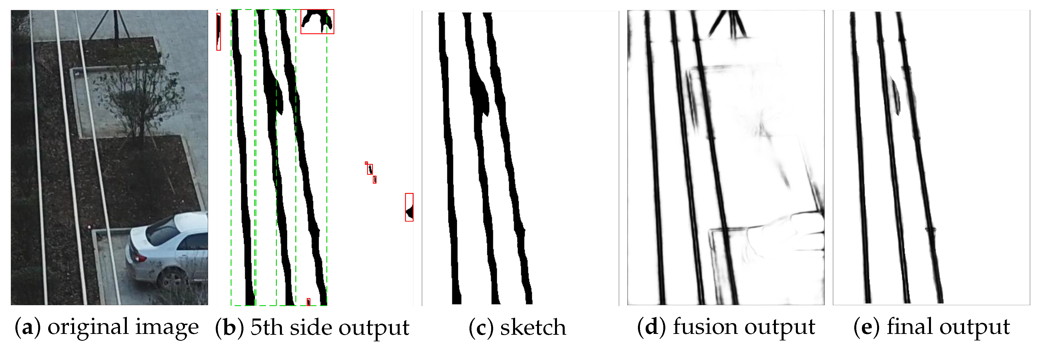
2.3. Structured Features

The output of the fusion layer combines multiscale cues to give relatively accurate results. However, there still are many noisy fragments in fusion output. Therefore, we exploit the structured priors of power lines to filter out noisy edges, which include length, size and orientation. Generally speaking, the orientations of power lines are distributed regularly, while noisy edges are presented in a mess. Besides, the size of each power line is similar, not extremely small or large. It can be noticed that power lines in a image exhibit uniform orientation, size and length. On the basis of the observation, we need to find a suitable method to extract the structured information of power lines from multi-level feature maps and combine it with the fusion output. Although the fusion output is relatively accurate compared with the results of traditional methods, it may be difficult to extract the structured features from it due to noisy background. Figure 2 exhibits the fine-to-coarse side outputs from the network. The shallower convolutional layer captures the detailed information, such as leaves, tiles and small objects, while the deeper convolutional layers give a slight glance of the image and perceive the salient structure in a global view. We can surprisingly observe that the side output of the fifth stage consists of clearest power line sketches with little noise. The conv layers with the largest stride in the fifth stage only give responses to objects with highest confidence, the detailed information such as tiles and leaves is ignored. Although the power lines in the fifth side output appear thick and inaccurately localized, it provides us rich information about structures, which can be fully exploited to reduce noise.

We extract structured features from the fifth side output with the aim of sweeping out isolated noisy fragments. Figure 3 displays the intermediate outputs in the process of structure extraction. First of all, the edge map of the fifth side output is binarized to calculate eight-connected regions. We can see from Figure 3b that there is several bounding boxes to cover each region, the number of pixels of each fragment is counted, then the orientation of each fragment is approximated by the long axis of the ellipse that has the same second-moments as the region. The length is estimated by the diagonal of bounding box. As mentioned above, the objects appear on the fifth side output are predicted by the network with the highest confidence. Therefore, we assume the fragment with the longest length as power line. The other fragments are determined to be kept or removed by the restrictions of area and orientation. The small fragments are filtered by area measurement:

$$K=are{a}_{Lmax}/area$$

(6)

where $are{a}_{Lmax}$ is the number of pixels of the longest fragment. If K exceeds a threshold $T_A$, it indicates the fragment is far smaller than standard one, so it is rejected as noise. Similarly, the fragments with messy directions are filtered by orientation measurement:

$$P=\left|\right|{\theta }_{Lmax}|-|\theta \left|\right|$$

(7)

where ${\theta }_{Lmax}$ is the orientation of the fragment with longest length. It is worth mentioning that $\theta$ is the angle between the fragment and the positive direction of the horizontal axis. The measurement takes both symmetric and parallel circumstances into consideration. If P is calculated beyond a threshold $T_{\theta }$, it suggests the fragment is messy and has completely distinct orientation, so it is rejected as noise. The fragment which satisfies both the two conditions is considered to be power line. For fear of filtering out short power lines, a looser threshold 1.5$T_A$ is adopted, but the threshold for orientation is stricter accordingly, which is set to be 0.5$T_{\theta }$. It means small fragment strictly parallel to the standard one is considered to be power line. As a result, any fragment which meets the requirement of ($T_A$, $T_{\theta }$) or (1.5$T_A$, 0.5$T_{\theta }$) is considered to be meaningful structure. Combining the two criteria, the clean edge map of fifth side output is obtained, which contains the sketch of power lines.

In conclusion, structured information can be exploited to reduce noise without losing the precision of localization. The sketch of power lines in Figure 3c is extracted using the above method from the binarized fifth side output. The power line pixels are considered to be within the sketch, so it is utilized as a mask to the fusion output to filter out noisy fragments. As a result, the edge map with accurate power line localization and clear background is obtained, which is shown in Figure 3e. Besides, the orientation and length of power line can be estimated by the sketch, which is substantially meaningful for the autonomous navigation of unmanned aerial vehicles.

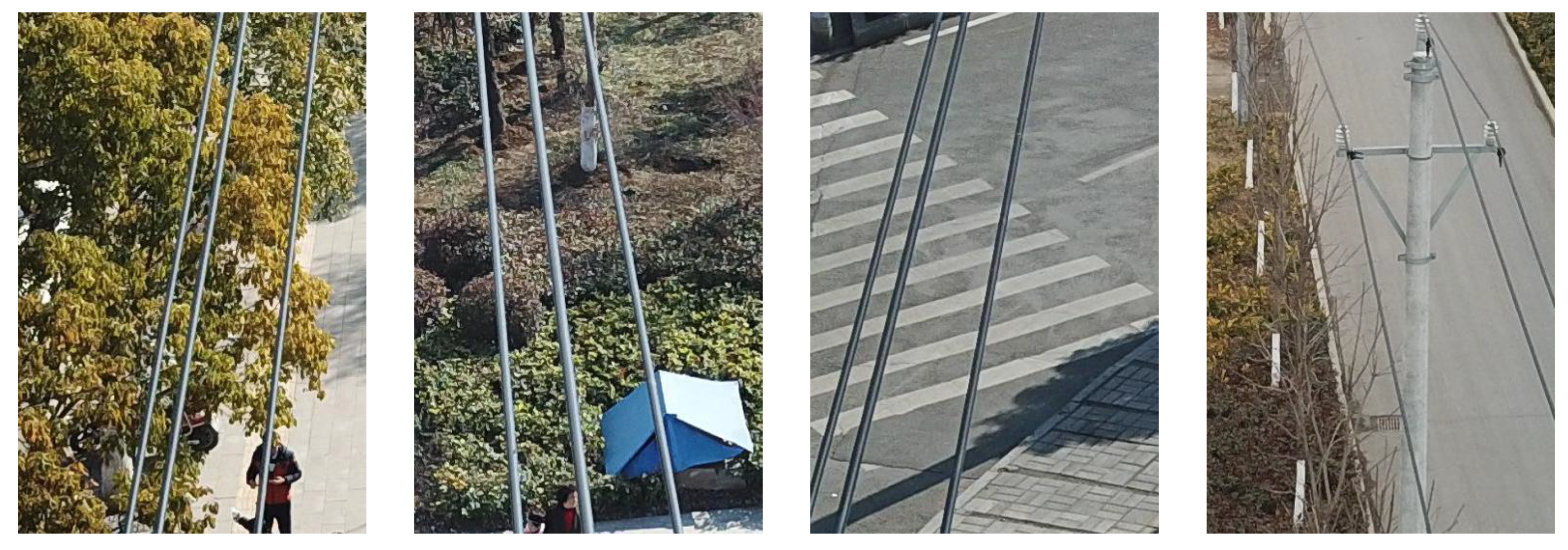
3. Power Line Datasets

For power line detection, large public datasets with pixel-wise annotations are scarce. As a result, most of the previous methods are developed on top of traditional edge detectors and evaluated on just a few images. However, the learning-based methods can hardly be developed for lack of well-annotated datasets for training and testing. In order to solve the problem, we release two power line detection datasets, power line dataset of urban scene which is named as PLDU and power line dataset of mountain scene which is named as PLDM. Some sample images from the two datasets are displayed in Figure 4 and Figure 5. Compared with images in PLDU dataset, the power lines in PLDM dataset are thinner due to the longer shooting distance and the backgrounds are usually less noisy which are mainly leaves and grasses. Specifically, the images in PLDU dataset are captured with UAV hovering above the power lines within ten meters. While the images in PLDM dataset are captured with the distance of more than thirty meters. In

Table 2. The detailed information about the two datasets used in the evaluation.

Dataset	Train	Test	maxDist
PLDU	453	120	0.0075
PLDM	237	50	0.0075

, we report the number of training and testing images in each dataset, along with the maximal tolerance of edge localization in evaluation. It is worth mentioning that the misalignment between manually labeled ground truth and real boundary is inevitable, so the parameter maxDist introduced in [26] is needed to reduce errors in evaluation. It is the fraction of image diagonal and used to compute minimum-cost correspondence between two boundary maps. When the distance between input pixel and human labelled pixel is within maxDist, the cost is proportional to their Euclidean distance. Otherwise, the cost is assigned a outlier cost for penalization. The two datasets are annotated with the same criterion, so the maximal tolerance of edge localization is set to 0.0075 for both datasets. As for data acquisition, all the original images are collected using DJI phantom 4 Pro under different weather conditions. Besides, we try to keep the background of images as varied as possible to prevent overfitting. The size of the original images is 3000 × 4000 pixels, which is too large to be ultilized directly. Therefore, the meaningful regions of uniform size 540 × 360 pixels are cropped from the original images to form the datasets.

To acquire pixel-level annotations, we adopt the publicly available semi-automatic boundary annotation tool ByLabel [27], in which edge fragments detected by EDLines [28] are selected by annotator and combined automatically. Compared with purely manual annotation, the semi-automatic annotation is much more accurate for the superiority of EDLines on edge localization. It is pointed out in [29] that edge learning based on CNN tends to be vulnerable to misaligned boundary labels due to the delicate structure of edges. When performing evaluation, even slight misalignment may lead to significant proportion of mismatches between ground truth and prediction. Although it is inevitable to produce the misalignments, we can greatly reduce them by using semi-automatic annotation tool, so that valid conclusion can be drawn from evaluation. For the task of power line detection, the boundary of power lines is concise and less controversial, so each image is annotated by only one researcher without the need to average different annotations. In this way, the faint edges like BSDS500 that may confuse the network can be avoided.

Data augmentation is recognized as a meaningful technique to improve performance in edge learning. Similar to the technique in [24], we rotate the images every 45 degrees, and then flip the images at each angle. Additionally, multiscale images are also proved to be useful for training, so we resize all the training images to scales 0.5 and 1.5. As a result, the augmented training set is 48 times larger than the original one.

The main advantage of the two datasets is that they are collected in real world using UAVs, not by synthetic ways. It has been experimented in [19] that training on synthetic data alone is not enough to reach the performance of models fine-tuned on real-world datasets. Besides, the power lines in our two datasets are varied in orientations, positions, lengths, widths with various backgrounds, which benefits us to develop learning-based methods for accurate power line detection. Temporarily, the PLDM dataset is relatively small for deep learning methods, so we only ultilize the its test set for across-dataset test. The PLDU dataset is adopted as main dataset for evaluation.

4. Experimental Results

In this section, we describe the implementation of the proposed method in detail and demonstrate the performance of our proposed method compared with baselines.

4.1. Implementation

We implement our network on the basis of the publicly available Caffe and build our method on top of VGG16. Considering the requirements of flexible deployment and real-time performance on onboard platform, not ResNet101 [30] but VGG16 is adopted as the backbone of our network. The parameters of each layer in the network are initialized by pre-trained VGG16 models on ImageNet. The weights of 1 × 1 conv layers in stage 1–5 are initialized from Gaussian distributions with zero mean and 0.01 standard deviation. The weights of fusion layer are initialized to 0.2. The remaining hyper-parameters settings are listed as follows: mini-batch size (10), loss-weight $a_m$ of side-output layers (1), weight decay (0.0002) and momentum (0.9), the number of training iterations (20 k), the parameter $\lambda$ in loss function (1.1), global learning rate (${10}^{-8}$) and will decay to one-tenth every 10 k iterations. It can be observed that the performance of $F_1$-measure is approximately the same when training process converges.

Then, the power line sketch containing structured features is extracted from the fifth side output using both area and orientation measurements. The thresholds $T_A$ and $T_{\theta }$ are set to 6 and 20, respectively. For each fusion output, the sketch is applied as a mask to filter out noisy fragments. The edge map is obtained with clear background and accurate power line localization. Finally, the standard non-maximum suppression in [26] is adopted to refine the detected edge map, making the boundary of power line one-pixel width for fair competition.

The final output is presented as edge probability map, in which the fainter edges are less likely to be the part of power lines, while the dark ones indicate stronger evidence of the existing of power lines. For evaluation, we refer to the boundary detection benchmark developed in BSDS500 dataset. The accuracy of power line detection is measured using four main criteria: $F_1$-measure of optimal dataset scale threshold (ODS), $F_1$-measure of optimal image scale threshold (OIS), false positive rate and precision-recall curve. We report the performance of our proposed method and baselines using the four criteria. At present, all the experiments are carried out on a single NVIDIA GeForce GTX 1070 GPU.

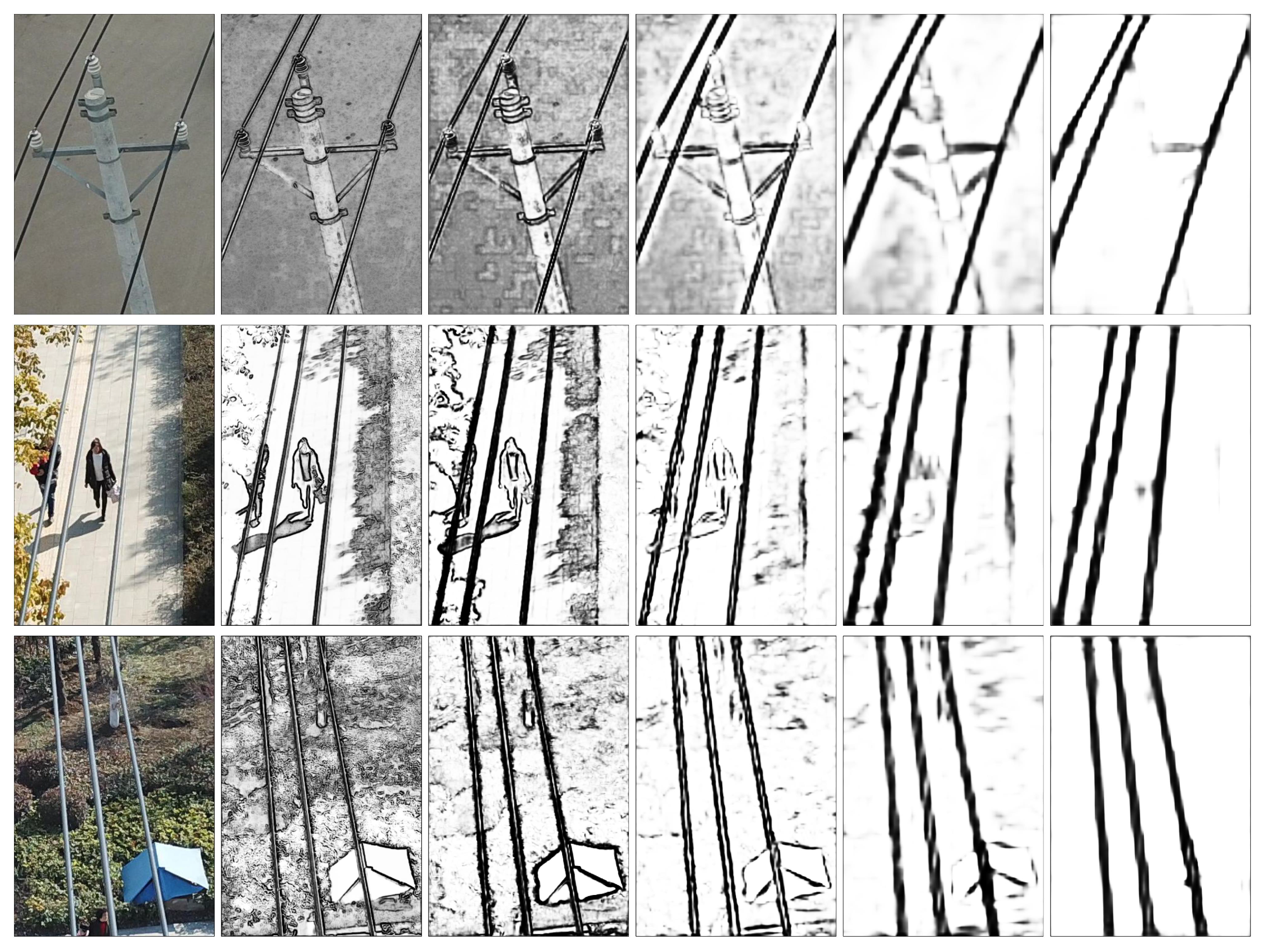
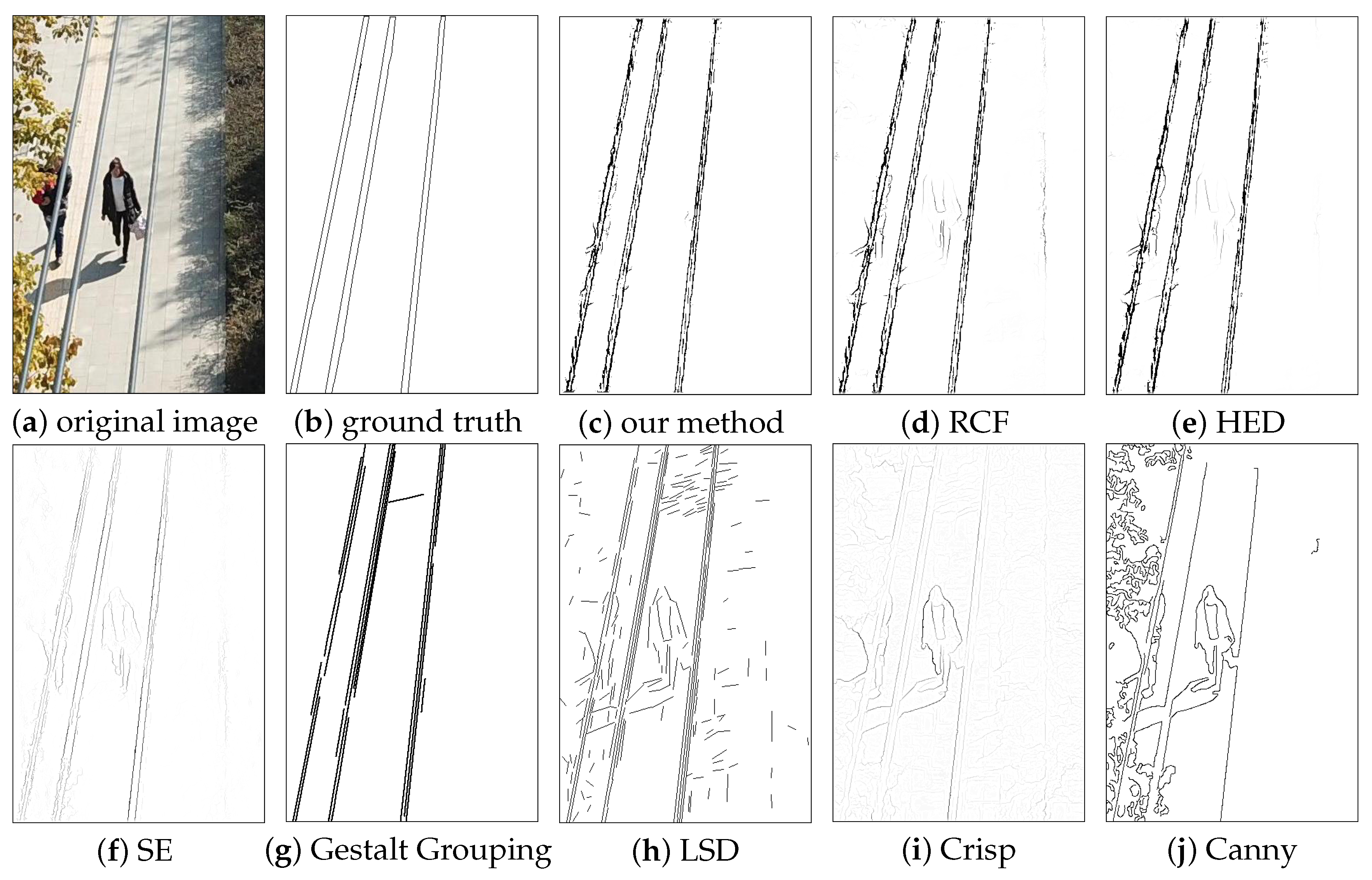
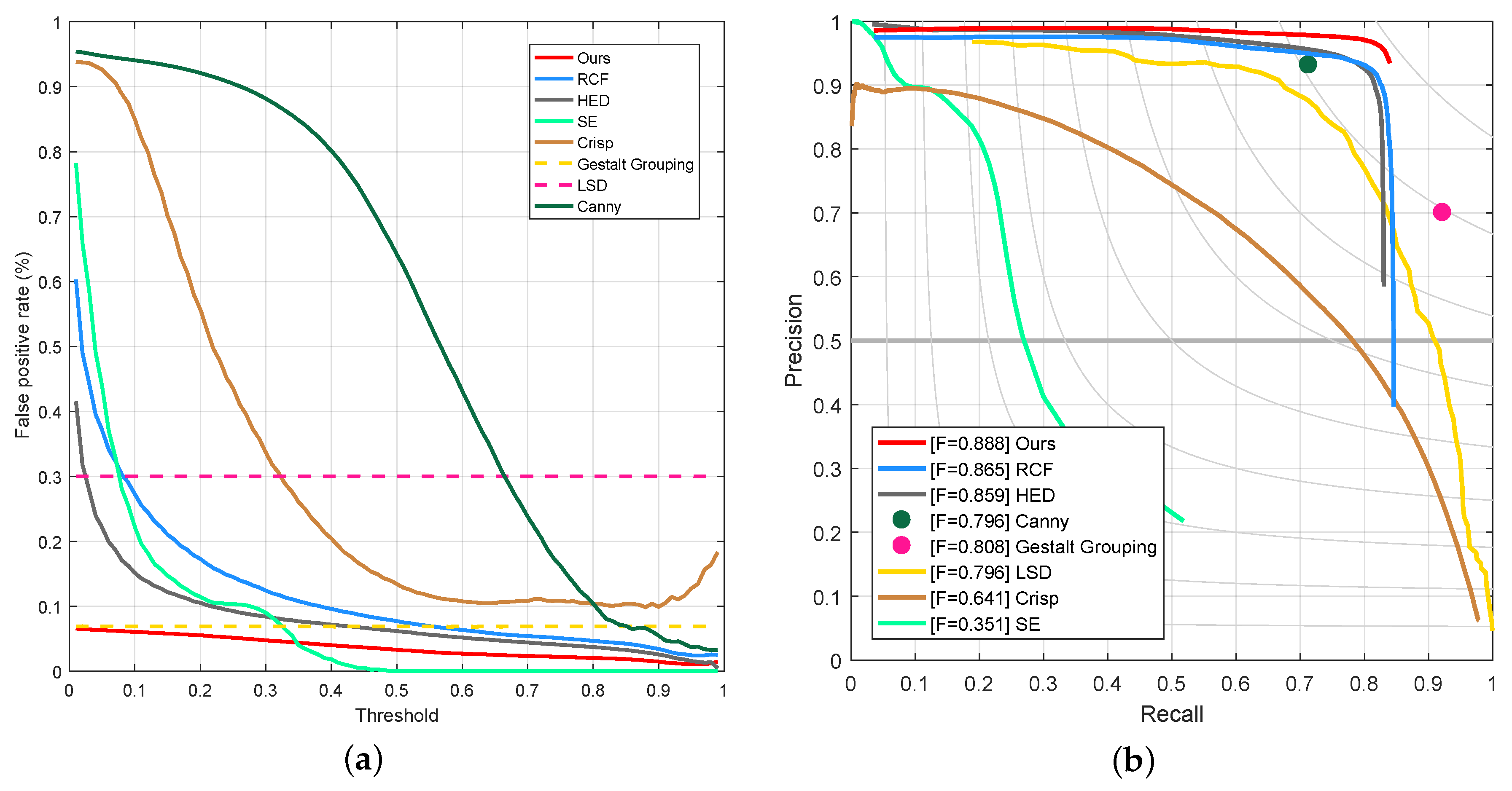
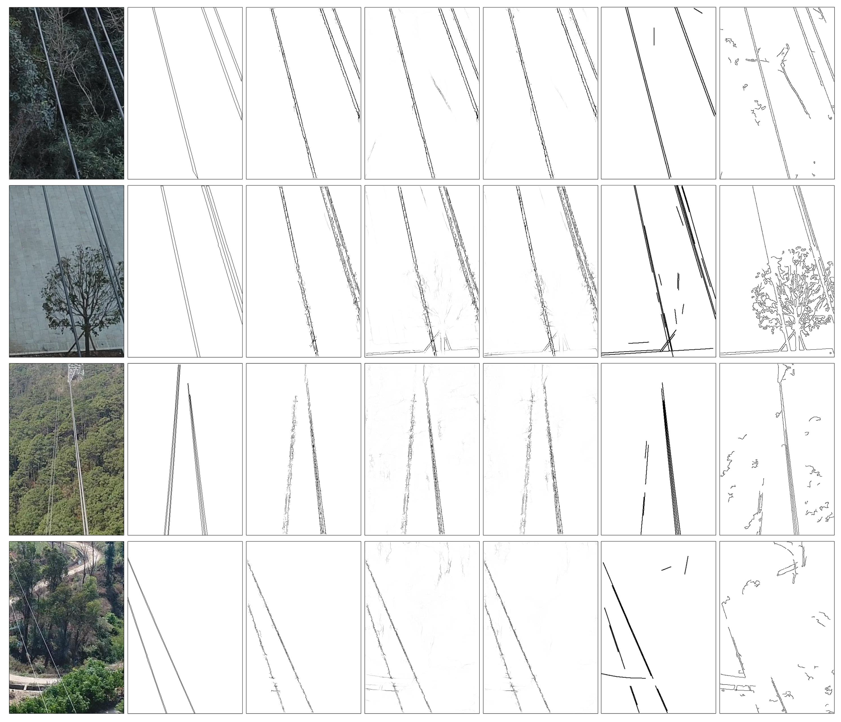
4.2. Experiments on PLDU Dataset

We adopt the training set of PLDU dataset for fine-tuning and obtain the trained model. Our method and the baselines are evaluated using the test set of PLDU dataset. In experiment, our proposed method is compared with classical Canny [31], LSD [32], Gestalt Grouping [33], Crisp Boundaries [34], SE [35], HED [24] and original RCF. It is worth mentioning that there are four different outputs of Gestalt Grouping method, following different gestalt restrictions. For the task of power line detection, we adopt the non-local alignments as baseline method.

Figure 6 gives an example image and its human annotation, as well as the results of different methods. We can observe that traditional edge detector Canny is sensitive to all boundaries without distinction. It produces edge map on top of local gradients and thresholds without applying any structured priors, so there exist many noisy fragments at human objects and leaves. LSD is specially designed for line detection which is also built on top of gradients and a contrario model. Compared with Canny, the line structure is more obvious with noise reduced but there still exist many isolated fragments. Gestalt Grouping is developed based on LSD using gestalt principles for non-local alignment. Obviously, its result is superior to LSD with higher precision at the cost of recall, most of the isolated fragments are filtered out with power lines kept. From the edge maps, we can see that the gradient-based methods, Canny, LSD and Gestalt Grouping, are sensitive to all kinds of local boundaries, even the unbalanced illumination on power lines, which leads to inaccurate edge localization. Crisp is built on top of mutual information of pixels, which has good performance on natural scene datasets. However, its performance is not satisfying on power line images due to complex background. From the edge map, we discover that Crisp tends to capture the boundary of salient object in image, such as human and get little response from power lines cluttered with textures. The learning-based method SE approaches the performance of ours, but it seems that SE predicts the edge map with less confidence, which can be observed from the lower pixel intensity of its result. As for the deep learning-based approaches, the original RCF produces fairly competitive results, but there still exist responses of nosiy objects, such as the boundaries of human. The overall performance of HED is similar to RCF, but it gives less false alarms. Compared with others, our method is less sensitive to noise and gives the accurate prediction with the clearest background. We can also notice that the noisy fragments are altered in our result due to the combination of structured information.

We can clearly find the superiority of our method to other baselines from Figure 7a. It is worth mentioning that the methods with binary outputs produce a horizontal line in the false positive rate graph. However, Canny is an exception because its threshold can be manually set from 0 to 1. Our method has the lowest false positive rate among other competitors when threshold is set to zero, and the curve remains relatively stable as the threshold increases. While, the false positive rates of other methods drop from higher values and the curves keep decreasing along threshold. It suggests that most of the noisy fragments in our results are eliminated by the use of structured information, the remaining pixels are predicted to be power lines with high confidence which share consistent intensity. When applied in practice, our method can detect accurate power lines with equally clear background at a random threshold within a large range. However, the performance of other methods varies greatly with threshold. For these methods, it’s hard to decide the optimal threshold to reach the trade-off between power lines and noisy fragments. As a result, our method is more promising to be exploited in real environment.

The overall performance of the methods is shown in Figure 7b. It should be noticed that the performance of methods with binary output is represented by a point in precision-recall curve. From the curves, we can observe that there is a large gap between the learning-based methods and traditional gradient-based methods. Especially when the background of images is complex, the learning-based methods perform much better than the traditional ones. Our proposed power line detection method achieves the superior performance of 0.914 ODS $F_1$-measure.

Table 3. The quantitative comparison with baselines on PLDU dataset, † means GPU time.

Method	ODS	OIS	FPS
Ours	0.914	0.938	15.6 ${}^{†}$
RCF	0.907	0.931	18.2 ${}^{†}$
HED	0.905	0.927	18.2 ${}^{†}$
SE	0.850	0.898	1.7
Gestalt Grouping	0.629	0.629	2.0
LSD	0.593	0.593	26.7
Crisp	0.535	0.622	0.3
Canny	0.466	0.643	22.4

gives the quantitative results. It’s worth mentioning that the methods with binary output are supposed to give equivalent OIS and ODS value. We can observe that our proposed method outperforms the baselines and achieves the best OIS and ODS $F_1$-measure on PLDU dataset. Moreover, the structured information extracted from the fifth side output is proved to be valid, which globally eliminates noisy fragments and improves the overall performance on PLDU dataset. The time consumption is also listed in Table 3, it has been presented that our method achieves a good trade-off between accuracy and efficiency.

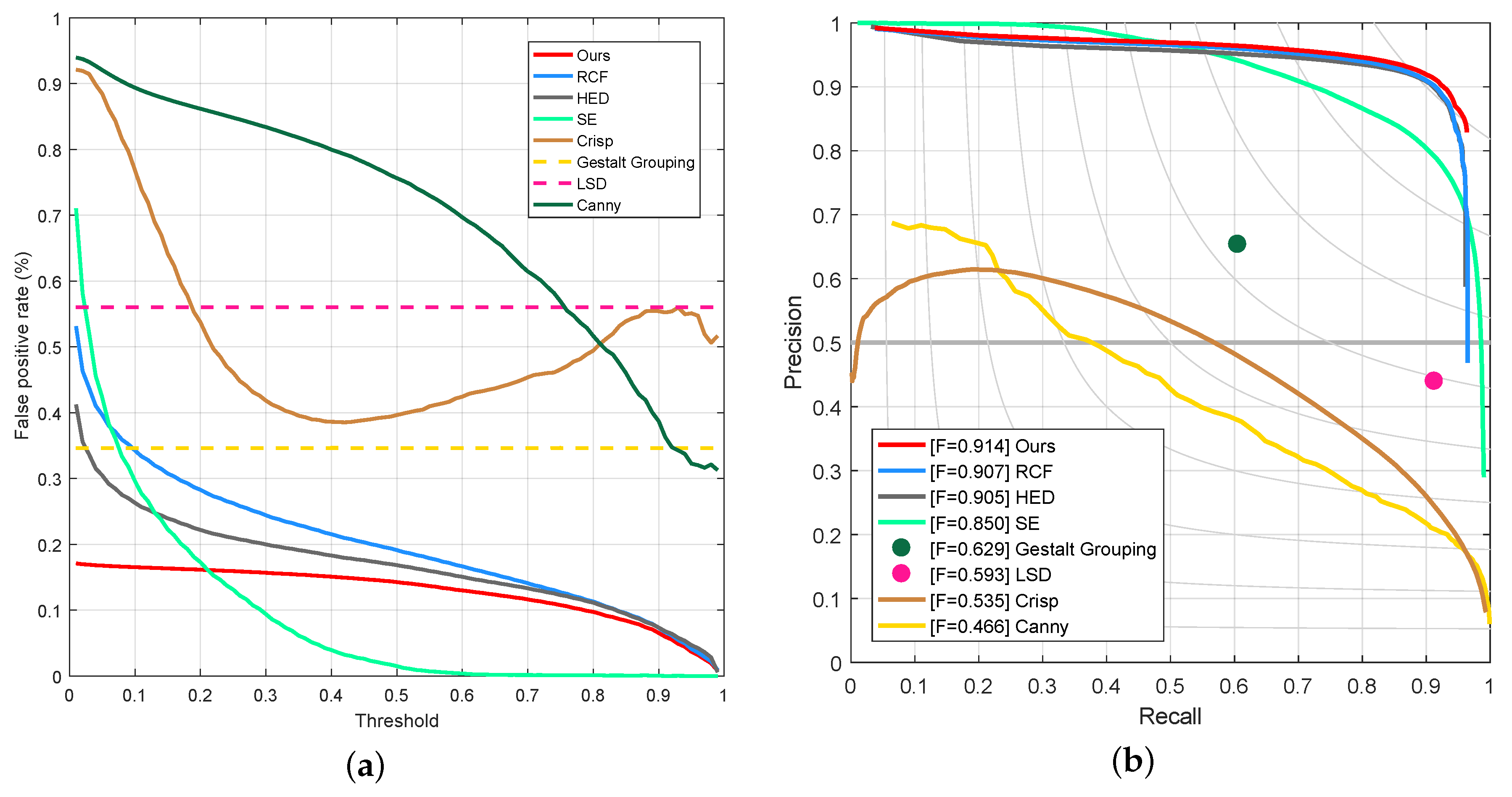
4.3. Experiments on PLDM Dataset

To further verify the effectiveness and robustness of our method, an across-dataset experiment is carried out. We evaluate our method and the baselines on the test set of PLDM dataset with model trained on the training set of PLDU dataset. Figure 8a gives the false positive rate curves, our method has the lowest false positive rate when threshold is below 0.3. As the threshold increases, all the responses in SE are regarded as negatives due to the faint edges produced by SE. Therefore, the curve of SE drops to zero when threshold exceeds 0.5. Our method is proved to be robust as threshold changes and it outputs the detected power lines with the clearest background. The precision-recall curve is shown in Figure 8b. From the precision-recall curves, we can find an interesting phenomenon that the precision-recall curve of our method is not as long as others and it drops slightly. It may suggest that our method has swept out most of the noisy fragments and demonstrates high precision even at a lower threshold. Besides, the performance is stable as the threshold changes within a large range. Although our method is evaluated on a totally different dataset, it remains superior to other methods, which demonstrates the robustness of our method.

The statistical results are displayed in

Table 4. The quantitative comparison with baselines on PLDM dataset, † means GPU time.

Method	ODS	OIS	FPS
Ours	0.888	0.902	15.6 ${}^{†}$
RCF	0.865	0.893	18.2 ${}^{†}$
HED	0.859	0.883	18.2 ${}^{†}$
SE	0.351	0.340	2.5
Gestalt Grouping	0.808	0.808	5.6
LSD	0.796	0.796	24.7
Crisp	0.641	0.752	0.3
Canny	0.796	0.866	20.6

. We can surprisingly find that the model of our method, HED and RCF learned on PLDU dataset can be well transferred to PLDM dataset, while SE performs badly on the across-dataset test. Similarly, we achieve the superior performance to other competitors. Gestalt grouping, LSD and Canny have the similar performance as the second echelon. It is mainly due to the fact that the images in PLDM dataset are less noisy and the gradients of power lines can be easily distinguished from the background by thresholds. Crisp still cannot identify power line pixels from insufficient mutual information, it may not be suitable for the detection of thin structures. SE with model trained on PLDU dataset is not able to capture the features of thinner lines in PLDM dataset, which brings about the sharp drop of performance on the test. Particularly, the performance of RCF is superior to HED, which demonstrates the effectiveness of using feature maps from all conv layers. Compared with RCF, the improvement of our method on ODS and OIS $F_1$-measure is significant, which proves the robustness of the structured information. As for efficiency, most of the methods exhibit consistent results with Table 3. However, Gestalt Grouping is an exception because its time consumption depends on the number of potential line segments. Although our method is not the most efficient, it produces superior results with competitive efficiency. More power line detection results are presented in Figure 9. It can be concluded that our proposed method achieves robust performance on two different power line datasets and can adapt to different environments with strong generalization ability.

5. Discussion

Power line detection is a key module in automated UAV inspection system, its accuracy and efficiency determine the performance of the whole system. In this paper, we propose to combine convolutional feature maps with structured information for power line detection. Our objective is to develop an accurate and efficient framework for the task so as to apply it on onboard platform. The experimental results on PLDU and PLDM datasets indicate that the proposed method outperforms the state-of-the-art methods.

The convolutional feature maps contain coarse-to-fine responses. The shallower convolutional layer captures the detailed information with accurate edge localization, while the deeper convolutional layer gives a slight glance of the image and perceives the salient structure in a global view. As described in Section 2, semantic boundary can be obtained in the fusion output by leveraging the multiscale feature maps. Unlike objects in natural images, power lines in different images share consistent structures, which can be fully exploited to reduce noise and boost performance. Therefore, we apply area and orientation measurements to the fifth side output to extract the sketch of power lines. The sketch is ultilized to filter out messy fragments in fusion output. As a result, our method gives accurate boundaries of power lines with the clearest background, which may benefit subsequent applications.

The extraction of structured information depends on the measurements described in Section 2.3. The fifth side output presents the area with the highest response in an image, so most of the noise is omitted. For some other objects with consistent structural features, the sketches can also be extracted from the fifth side output using specified principles. Therefore, the idea can be applied to other similar applications, and not limited to power line detection.

To find out the contribution of each component, we conduct an ablation study for different combinations of the fifth side output, structured features and the fusion output. To validate the effect of the structured features, we conduct an experiment to directly apply the fifth side output as a mask to the fusion output, denoted as fusion+side5 for short. Similarly, the structure-aware mask from the fifth side output (denoted as side5+SF) is used directly as output to prove the effect of the fusion output. Besides, an extra experiment is conducted that structured constraints are applied to the fusion output instead of the fifth side output (denoted as fusion+SF).

The results are summarized in

Table 5. Experiments on two datasets for ablation study.

Method	PLDU		PLDM
	ODS	OIS	ODS	OIS
fusion+side5	0.909	0.933	0.871	0.895
side5+SF	0.725	0.736	0.689	0.693
fusion+SF	0.909	0.934	0.880	0.899
full	0.914	0.938	0.888	0.902

. Compared with original RCF, both the fifth side output and the structured features contribute to the improvement in performance. The fifth side output contains the coarsest boundary of objects and the noise is highly limited, so it can be adopted to filter out noise in the fusion output. Similarly, the structured features to capture line segments are proved to be useful in the task even if it is applied directly on the fusion output. Although it seems in Figure 2 that the fifth side output alone presented good performance, the power lines in it appear thick and inaccurately localized. As a result, the fifth side output with structured constraints performs worse than the original RCF. In conclusion, extracting structured features from the fifth side output and then applying the structure-aware mask to the fusion output further boosts the performance. It produces accurate power line detection results with clear background and precise edge localization.

Although our method achieves desirable results on two datasets, there are still certain limitations. As mentioned above, the extraction of structured information relies on the quality of the fifth side output. Assuming that the responses from noise occupy a dominant position or little response can be found in the fifth side output, the process of structure extraction may be greatly affected. To solve this, we will focus on the continuity of power lines in adjacent frames of flight videos in future work. Combining the continuity and contextual information, the power line detection framework will be more robust in real environments. In addition, we will continue to update and expand the two datasets, collecting more power line images that reflect real-world conditions. Furthermore, the whole method will be ported to onboard platform NVIDIA Jetson TX2 later on.

6. Conclusions

In this paper, we introduce a new method which exploits deep-supervised neural network and structured features, for accurate power line detection using UAVs. Besides, we release two power line detection datasets with pixel-level annotations (PLDU and PLDM datasets) for evaluation. Leveraging hierarchical and structured features, our method produces both accurate and efficient results, which makes it possible to be applied in practice on a UAV onboard platform. In the future, we intend to explore the effectiveness of the continuity and contextual information in frames of flight video, which may further improve the robustness of our method. The datasets and pre-computed results are available at https://github.com/SnorkerHeng/PLD-UAV.

References

1. Matikainen, L.; Lehtomäki, M.; Ahokas, E. Remote sensing methods for power line corridor surveys. ISPRS J. Photogramm. Remote Sens. 2016, 119, 10–31. [Google Scholar] [CrossRef] [Green Version]
2. Zhu, L.; Hyyppä, J. Fully-automated power line extraction from airborne laser scanning point clouds in forest areas. Remote Sens. 2014, 6, 11267–11282. [Google Scholar] [CrossRef]
3. Wang, Y.; Chen, Q.; Liu, L.; Zheng, D. Supervised classification of power lines from airborne LiDAR data in urban areas. Remote Sens. 2017, 9, 771. [Google Scholar] [CrossRef]
4. Guan, H.; Yu, Y.; Li, J.; Ji, Z.; Zhang, Q. Extraction of power-transmission lines from vehicle-borne lidar data. Int. J. Remote Sens. 2016, 37, 229–247. [Google Scholar] [CrossRef]
5. Yan, G.; Li, C.; Zhou, G.; Zhang, W.; Li, X. Automatic extraction of power lines from aerial images. IEEE Geosci. Remote Sens. Lett. 2007, 4, 387–391. [Google Scholar] [CrossRef]
6. Chen, Y.; Li, Y.; Zhang, H. Automatic power line extraction from High resolution remote sensing imagery based on an improved radon transform. Pattern Recognit. 2016, 49, 174–186. [Google Scholar] [CrossRef]
7. Li, Z.; Liu, Y.; Walker, R.; Hayward, R.; Zhang, J. Towards automatic power line detection for a UAV surveillance system using pulse coupled neural filter and an improved Hough transform. Mach. Vis. Appl. 2010, 21, 677–686. [Google Scholar] [CrossRef]
8. Candamo, J.; Kasturi, R.; Goldgof, D.; Sarkar, S. Detection of thin lines using low-quality video from low-altitude aircraft in urban settings. IEEE Trans. Aerosp. Electron. Syst. 2009, 45, 937–949. [Google Scholar] [CrossRef]
9. Song, B.; Li, X. Power line detection from optical images. Neurocomputing 2014, 129, 350–361. [Google Scholar] [CrossRef]
10. Luo, X.; Zhang, J.; Cao, X. Object-aware power line detection using color and near-infrared images. IEEE Trans. Aerosp. Electron. Syst. 2014, 50, 1374–1389. [Google Scholar] [CrossRef]
11. Zhang, Y.; Yuan, X.; Li, W.; Chen, S. Automatic power line inspection using UAV images. Remote Sens. 2017, 9, 824. [Google Scholar] [CrossRef]
12. Zhang, Y.; Yuan, X.; Fang, Y.; Chen, S. UAV low altitude photogrammetry for power line inspection. ISPRS Int. J. Geo-Inf. 2017, 6, 14. [Google Scholar] [CrossRef]
13. Arbeláez, P.; Maire, M.; Fowlkes, C.; Malik, J. From contours to regions: An empirical evaluation. In Proceedings of the IEEE Conference on Computer Vision and Pattern Recognition (CVPR), Miami, FL, USA, 20–25 June 2009; pp. 2294–2301. [Google Scholar]
14. Arbeláez, P.; Maire, M.; Fowlkes, C.; Malik, J. Contour detection and hierarchical image segmentation. IEEE Trans. Pattern Anal. Mach. Intell. 2011, 33, 898–916. [Google Scholar] [CrossRef]
15. Shen, W.; Wang, X.; Wang, Y.; Xiang, B. DeepContour: A deep convolutional feature learned by positive- sharing loss for contour detection. In Proceedings of the IEEE Conference on Computer Vision and Pattern Recognition (CVPR), Boston, MA, USA, 7–12 June 2015; pp. 3982–3991. [Google Scholar]
16. Bertasius, G.; Shi, J.; Torresani, L. DeepEdge: A multi-scale bifurcated deep network for top-down contour detection. In Proceedings of the IEEE Conference on Computer Vision and Pattern Recognition (CVPR), Boston, MA, USA, 7–12 June 2015; pp. 4380–4389. [Google Scholar]
17. Yang, J.; Price, B.; Cohen, S. Object Contour Detection with a Fully Convolutional Encoder-Decoder Network. In Proceedings of the IEEE Conference on Computer Vision and Pattern Recognition (CVPR), Las Vegas, NV, USA, 26 June–1 July 2016; pp. 193–202. [Google Scholar]
18. Maninis, K.K.; Pont-Tuset, J.; Arbeláez, P. Convolutional oriented boundaries: From image segmentation to high-level tasks. IEEE Trans. Pattern Anal. Mach. Intell. 2018, 40, 819–833. [Google Scholar] [CrossRef]
19. Madaan, R.; Maturana, D.; Scherer, S. Wire detection using synthetic data and dilated convolutional networks for unmanned aerial vehicles. In Proceedings of the IEEE International Conference on Intelligent Robots and Systems (IROS), Vancouver, BC, Canada, 24–28 September 2017; pp. 3487–3494. [Google Scholar]
20. Chen, L.C.; Papandreou, G.; Kokkinos, I. Deeplab: Semantic image segmentation with deep convolutional nets, atrous convolution, and fully connected CRFs. IEEE Trans. Pattern Anal. Mach. Intell. 2016, 40, 834–848. [Google Scholar] [CrossRef]
21. Simonyan, K.; Zisserman, A. Very deep convolutional networks for large-scale image recognition. In Proceedings of the International Conference on Learning Representations (ICLR), San Diego, CA, USA, 7–9 May 2015. [Google Scholar]
22. Liu, Y.; Cheng, M.-M.; Hu, X. Richer convolutional features for edge detection. In Proceedings of the IEEE Conference on Computer Vision and Pattern Recognition (CVPR), Honolulu, HI, USA, 21–26 July 2017; pp. 5872–5881. [Google Scholar]
23. Long, J.; Shelhamer, E.; Darrell, T. Fully convolutional networks for semantic segmentation. In Proceedings of the IEEE Conference on Computer Vision and Pattern Recognition (CVPR), Boston, MA, USA, 7–12 June 2015; pp. 3431–3440. [Google Scholar]
24. Xie, S.; Tu, Z. Holistically-nested edge detection. Int. J. Comput. Vis. 2017, 125, 3–18. [Google Scholar] [CrossRef]
25. Martin, D.; Fowlkes, C.; Tal, D. A database of human segmented natural images and its application to evaluating segmentation algorithms and measuring ecological statistics. In Proceedings of the IEEE International Conference on Computer Vision, Vancouver, BC, Canada, 8–12 July 2001; pp. 416–423. [Google Scholar]
26. Martin, D.R.; Fowlkes, C.C.; Malik, J. Learning to detect natural image boundaries using local brightness, color, and texture cues. IEEE Trans. Pattern Anal. Mach. Intell. 2004, 26, 530–549. [Google Scholar] [CrossRef]
27. Qin, X.; He, S.; Zhang, Z.; Dehghan, M. ByLabel: A Boundary Based Semi-Automatic Image Annotation Tool. In Proceedings of the IEEE Winter Conference on Applications of Computer Vision (WACV), Lake Tahoe, NV, USA, 12–15 March 2018; pp. 1804–1813. [Google Scholar]
28. Akinlar, C.; Topal, C. EDLines: A real-time line segment detector with a false detection control. Pattern Recognit. Lett. 2011, 32, 1633–1642. [Google Scholar] [CrossRef]
29. Yu, Z.; Liu, W.; Zou, Y. Simultaneous Edge Alignment and Learning. arXiv 2018, arXiv:1808.01992. [Google Scholar]
30. He, K.; Zhang, X.; Ren, S.; Sun, J. Deep residual learning for image recognition. In Proceedings of the IEEE Conference on Computer Vision and Pattern Recognition (CVPR), Las Vegas, NV, USA, 26 June–1 July 2016; pp. 770–778. [Google Scholar]
31. Canny, J. A computational approach to edge detection. IEEE Trans. Pattern Anal. Mach. Intell. 1986, 6, 679–698. [Google Scholar] [CrossRef]
32. Von Gioi, R.G.; Jakubowicz, J.; Morel, J.M. LSD: A fast line segment detector with a false detection control. IEEE Trans. Pattern Anal. Mach. Intell. 2010, 32, 722–732. [Google Scholar] [CrossRef]
33. Rajaei, B.; von Gioi, R.G. Gestaltic Grouping of Line Segments. Image Process. Line 2018, 37–50. [Google Scholar] [CrossRef]
34. Isola, P.; Zoran, D.; Krishnan, D. Crisp boundary detection using pointwise mutual information. In Proceedings of the European Conference on Computer Vision (ECCV), Zurich, Switzerland, 6–12 September 2014; pp. 799–814. [Google Scholar]
35. Dollár, P.; Zitnick, C.L. Fast edge detection using structured forests. IEEE Trans. Pattern Anal. Mach. Intell. 2015, 37, 1558–1570. [Google Scholar] [CrossRef]
Figure 1. The structure of our power line detection network. The side outputs are generated by combining all the convolutional feature maps in each stage, which become coarser as the stride becomes larger. Exploiting the structured features, the final output presents excellent performance.
Remotesensing 11 01342 g001
Figure 2. Some examples of the fine-to-coarse side outputs from the network. From left to right: the original inputs, the feature maps extracted from the first side output to the fifth side output.
Remotesensing 11 01342 g002
Figure 3. The intermediate outputs in the process of structure extraction.
Remotesensing 11 01342 g003
Figure 4. Example images of power lines in PLDU dataset.
Remotesensing 11 01342 g004
Figure 5. Example images of power lines in PLDM dataset.
Remotesensing 11 01342 g005
Figure 6. Power line detection results on a sample image from PLDU dataset. From (aj): Original, Ground Truth, Ours, RCF, HED, SE, Gestalt Grouping, LSD, Crisp, Canny.
Remotesensing 11 01342 g006
Figure 7. The evaluation results on PLDU dataset. Our proposed method achieves the lowest false positive rate and superior F 1 -measure (ODS = 0.914) compared with baselines. (a) The false positive rate curves at different thresholds on PLDU dataset; (b) The precision-recall curves on PLDU dataset.
Remotesensing 11 01342 g007
Figure 8. The evaluation results on PLDM dataset. Our proposed method achieves superior F 1 -measure (ODS = 0.888) compared with baselines. (a) The false positive rate curves at different thresholds on PLDM dataset; (b) The precision-recall curves on PLDM dataset.
Remotesensing 11 01342 g008
Figure 9. Additional power line detection results are presented. The first two row images are from PLDU dataset, the last two row images are from PLDM dataset. From left to right: original image, ground truth, our method, RCF, HED, Gestalt Grouping and Canny.
Remotesensing 11 01342 g009