Building Instance Change Detection from Large-Scale Aerial Images using Convolutional Neural Networks and Simulated Samples


Abstract
:
1. Introduction
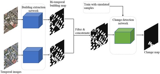
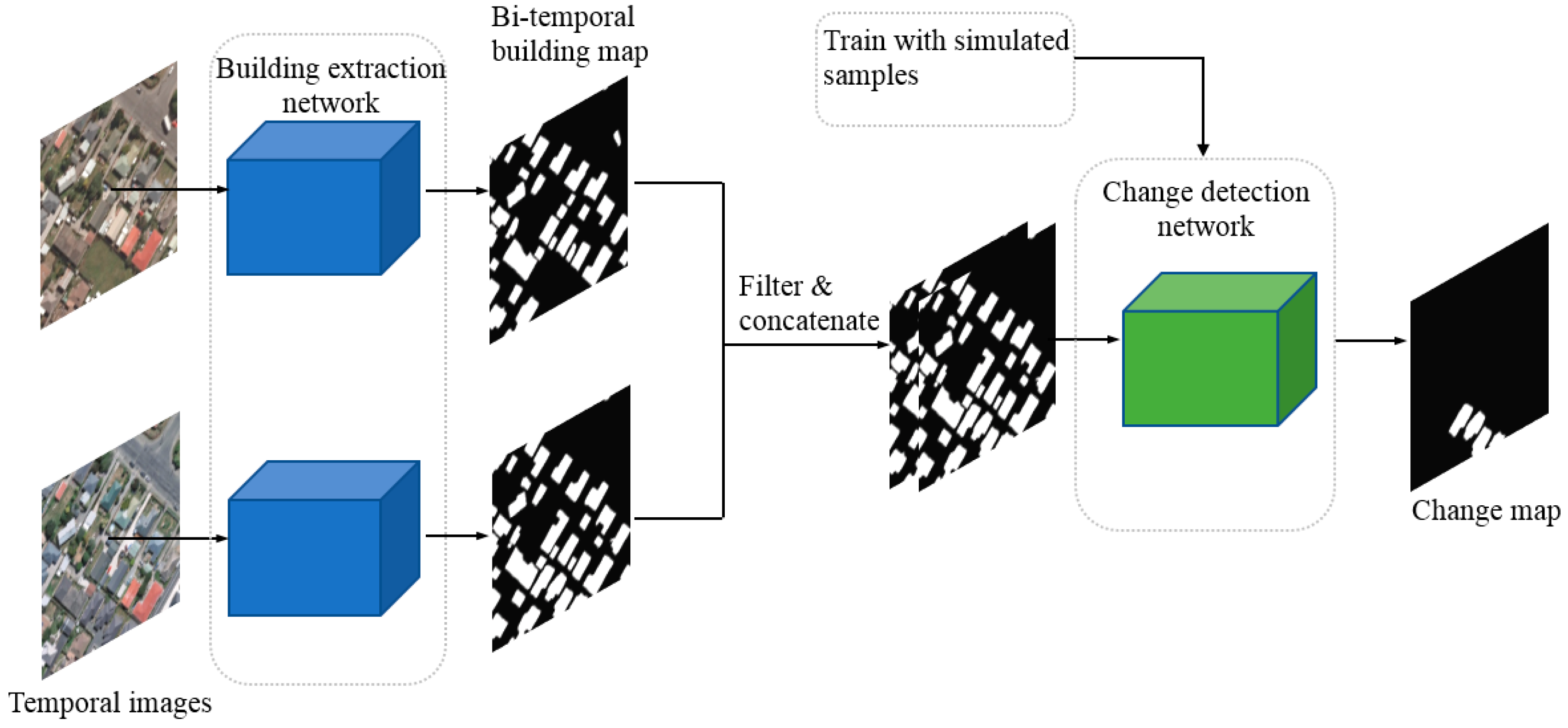
2. Methodology
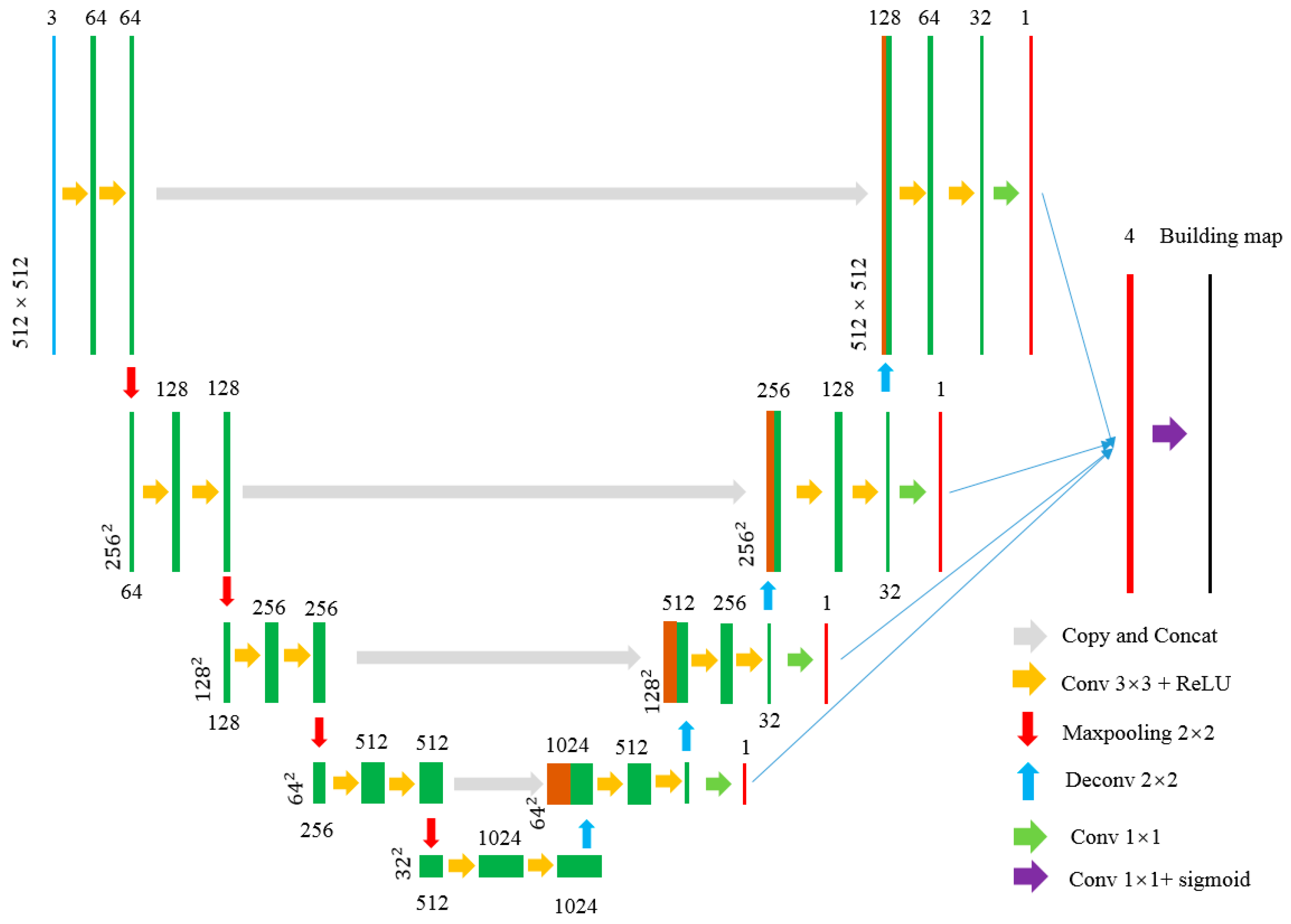
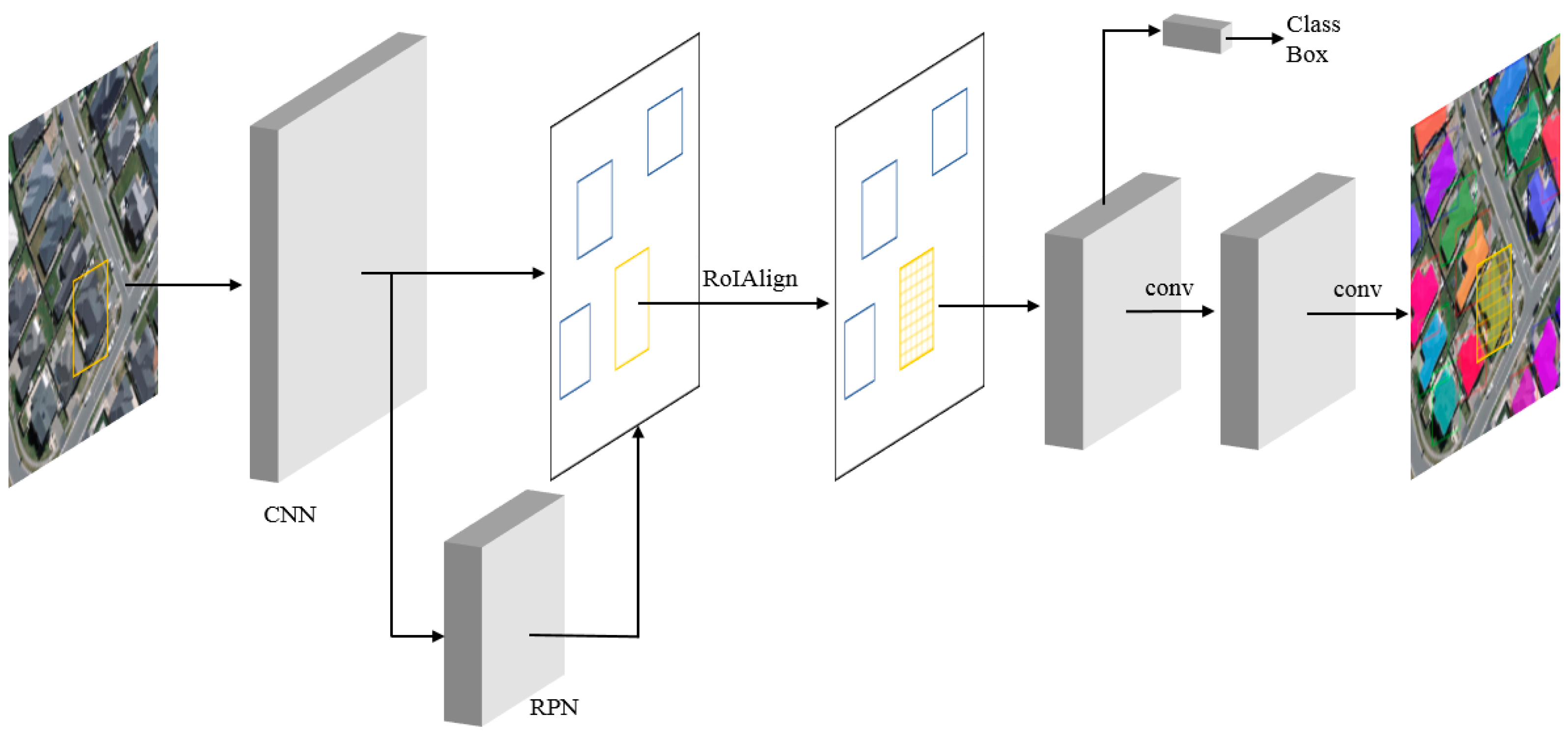
2.1. Building Extraction Network
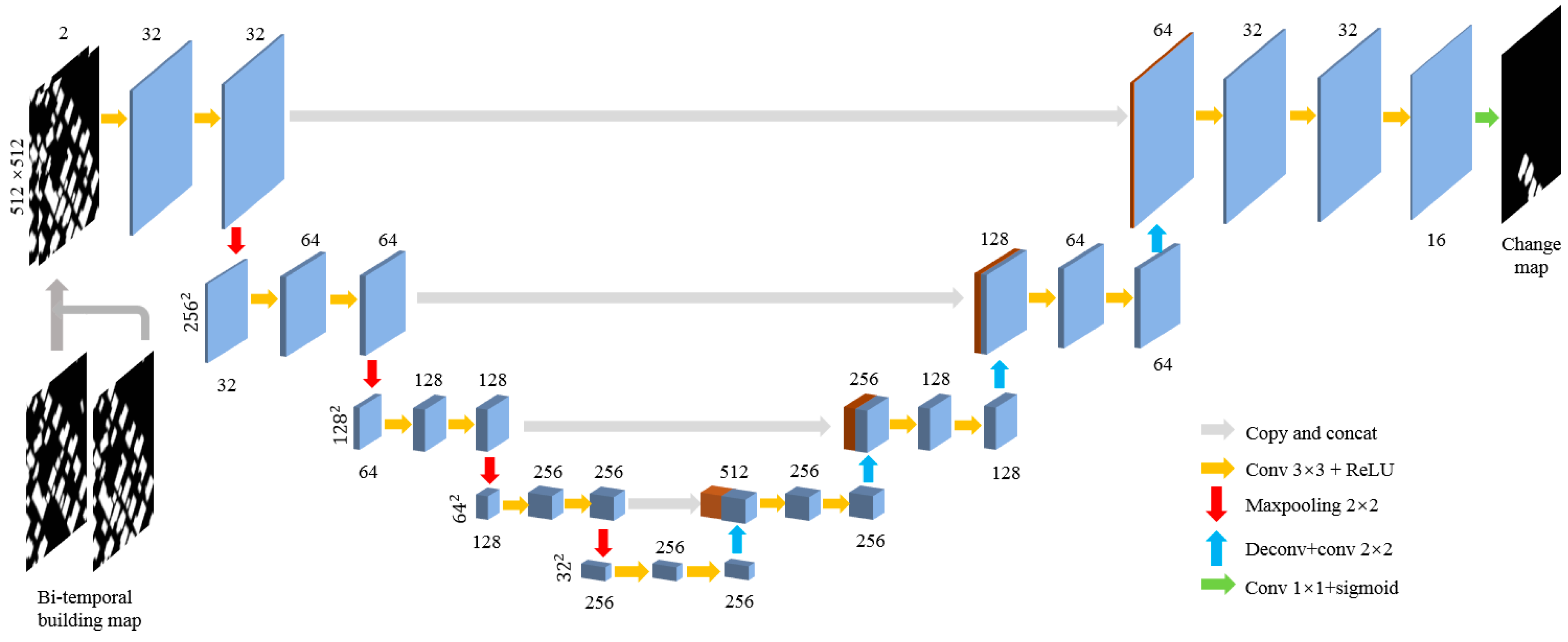
2.2. Self-Trained Building Change Detection Network
3. Experiments and Analysis
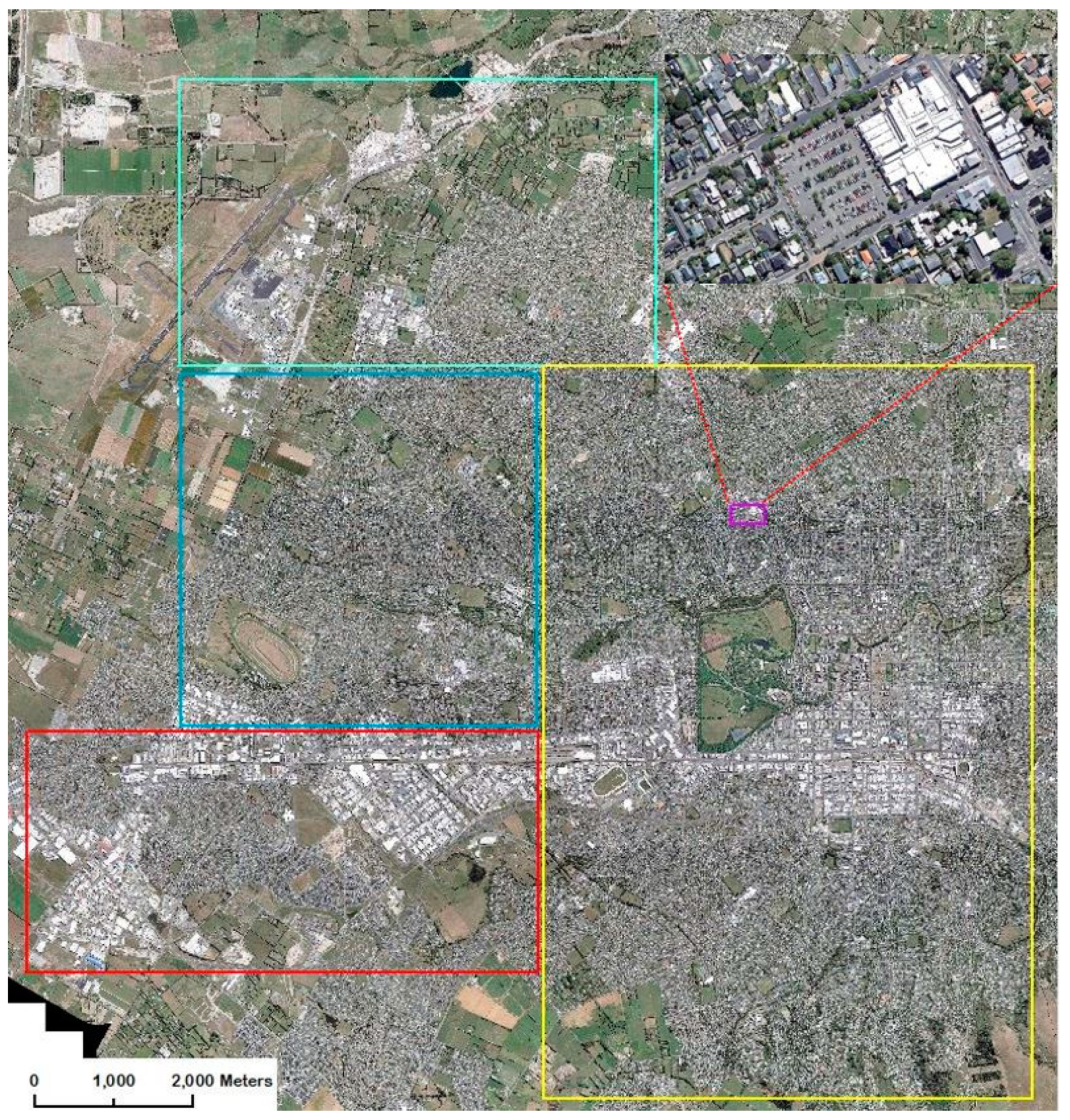
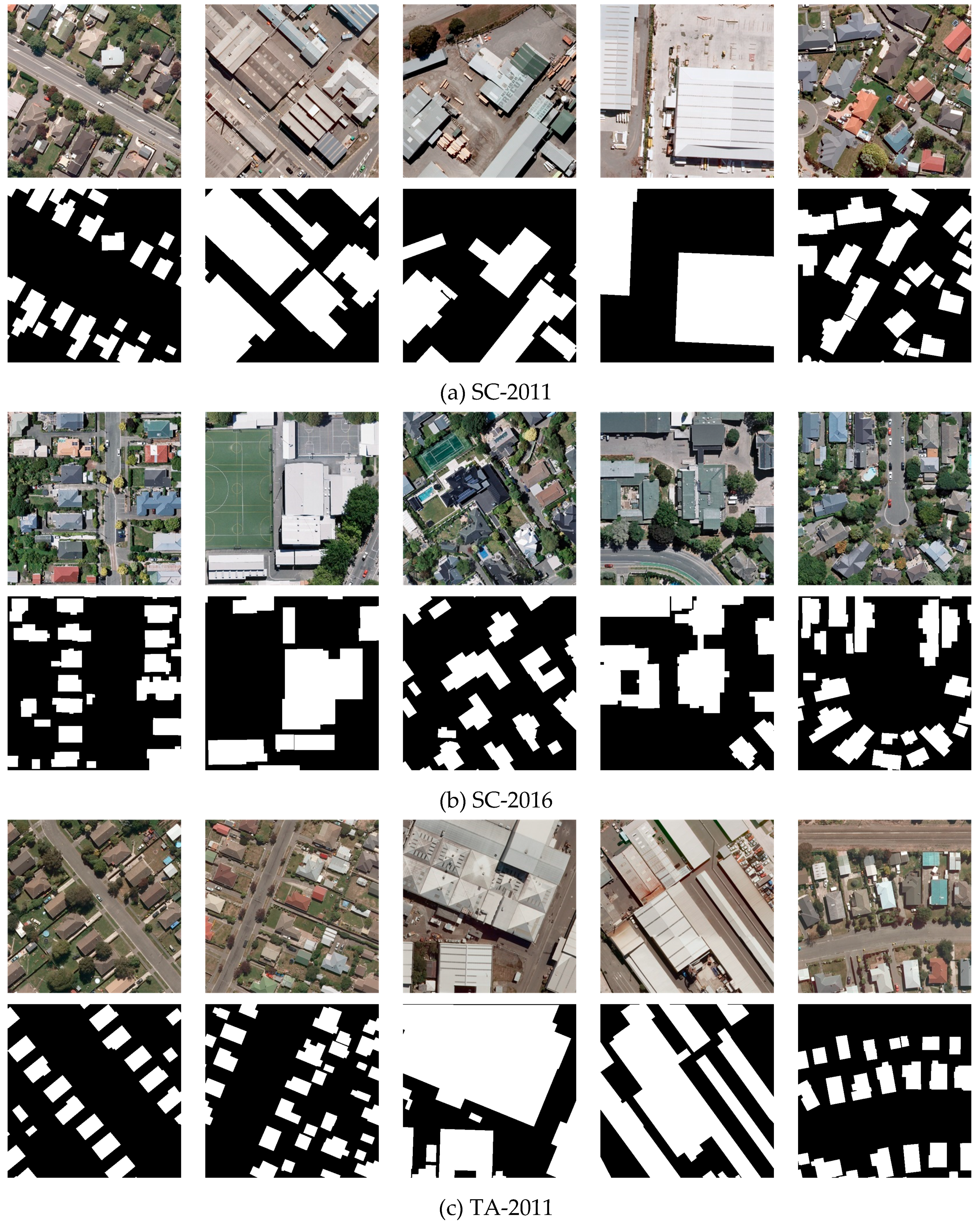
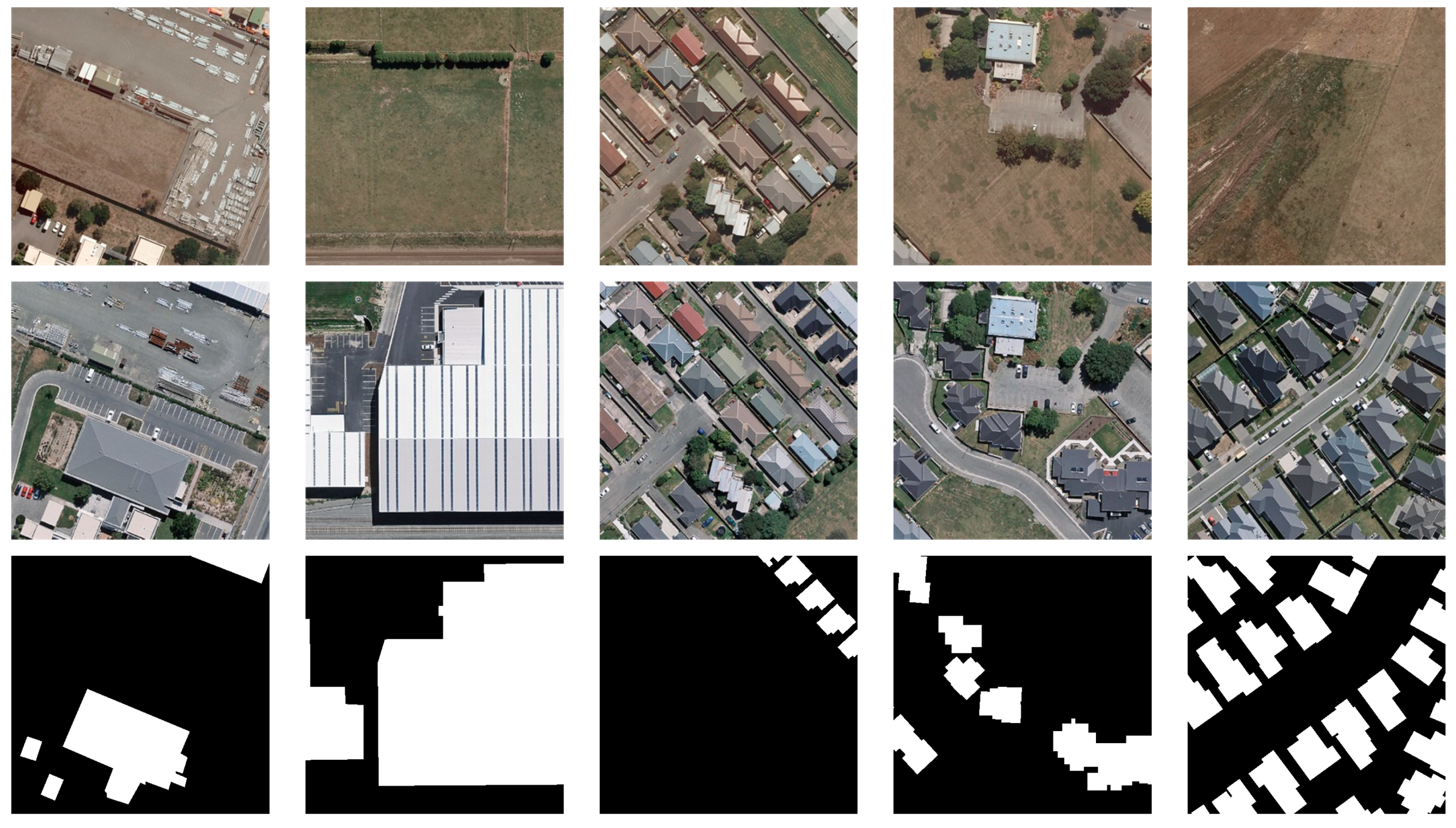
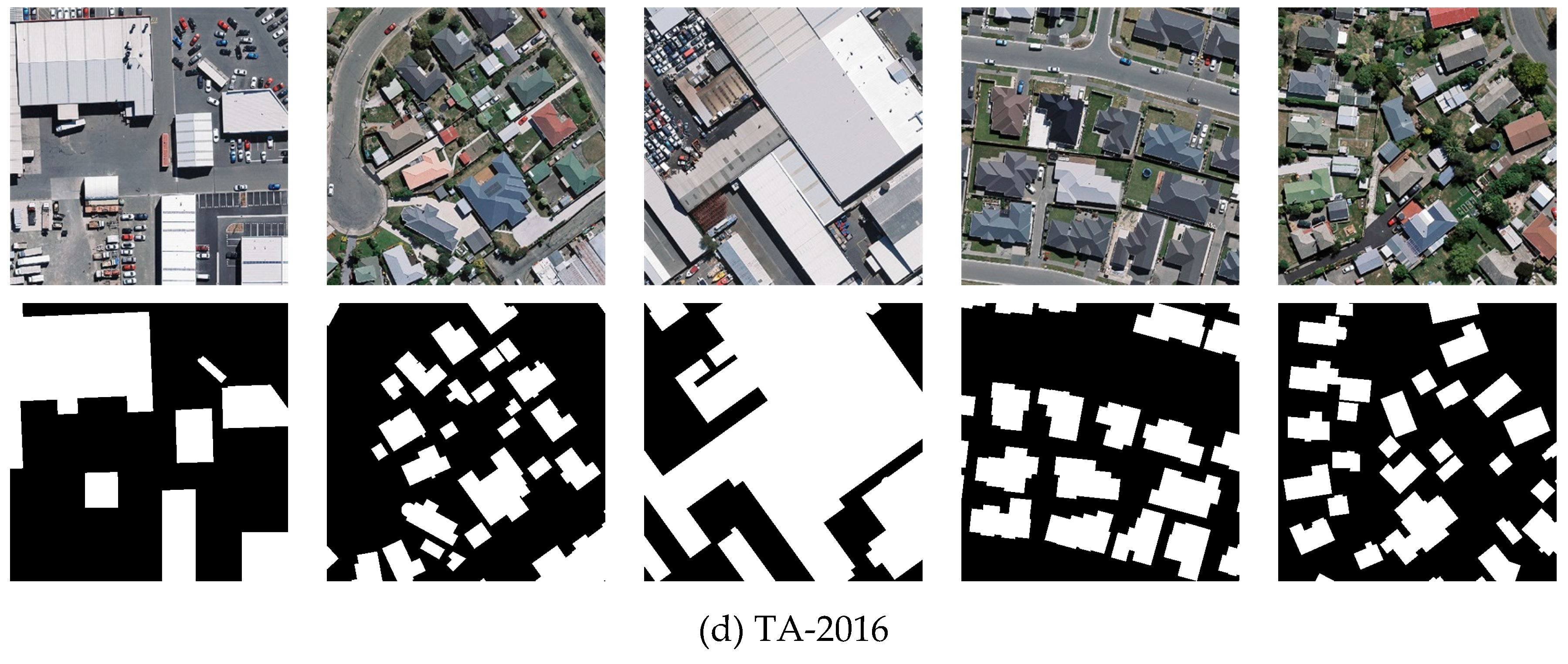
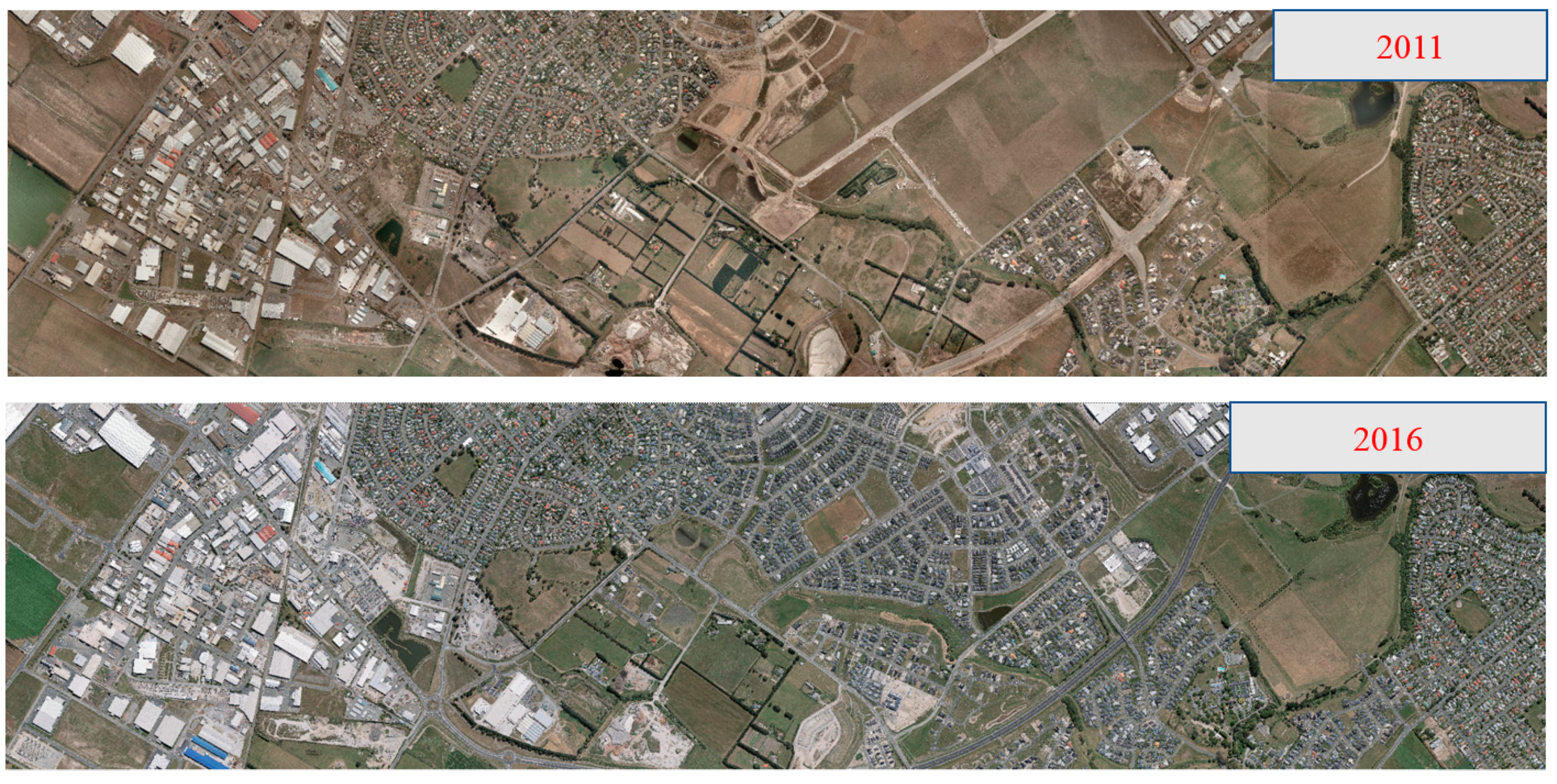
3.1. Data Set and Evaluation Measures
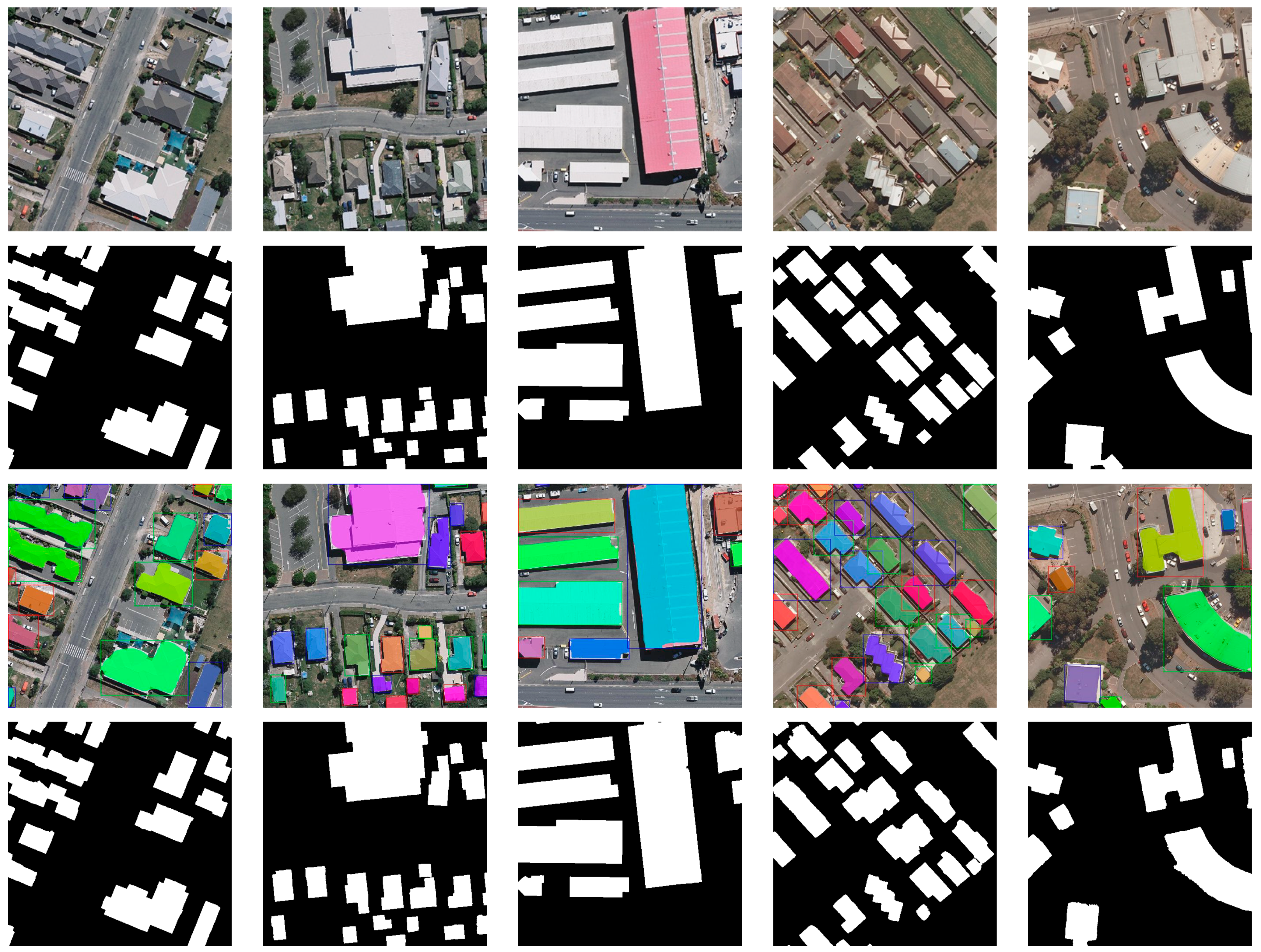
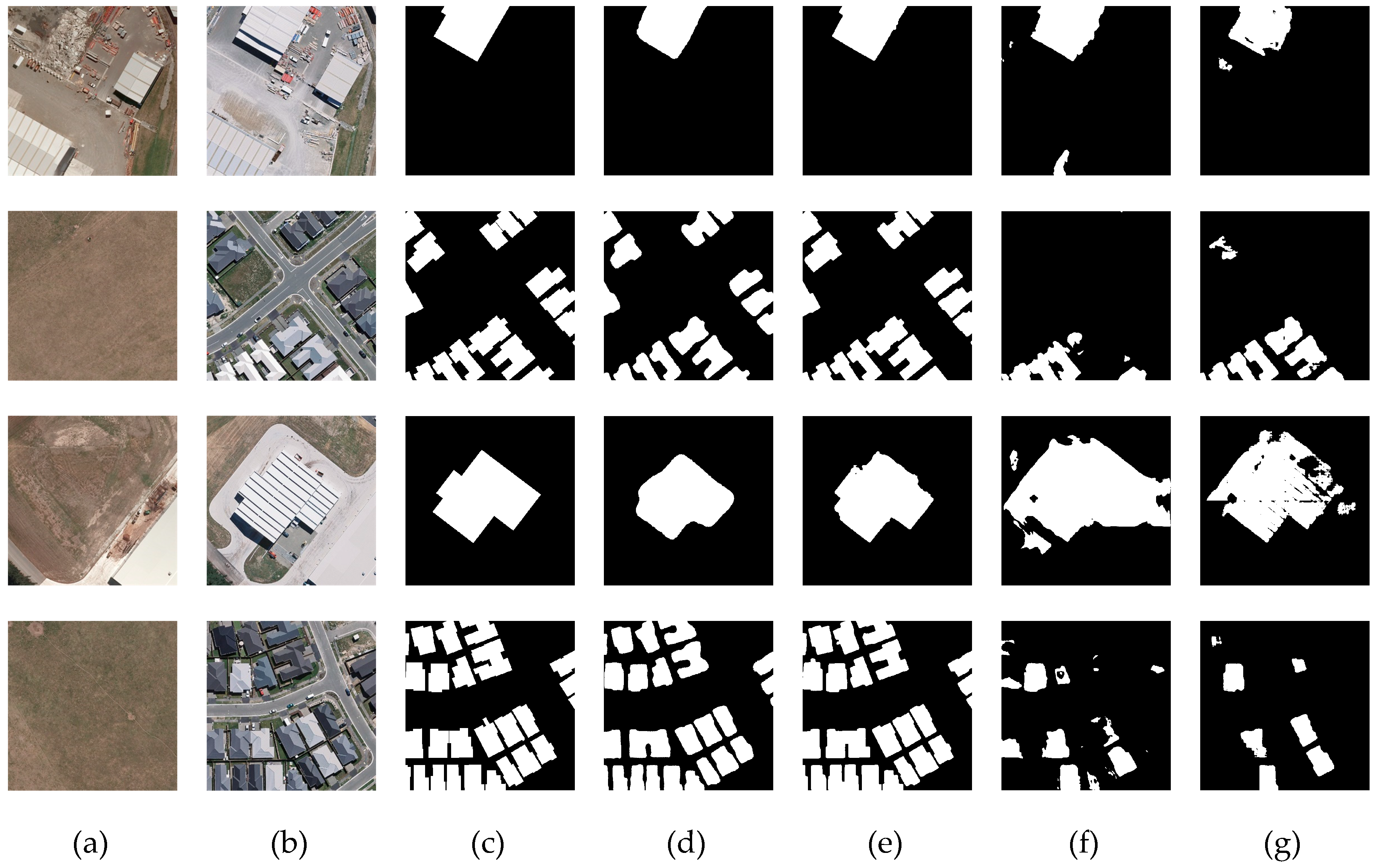
3.2. Building Extraction Results
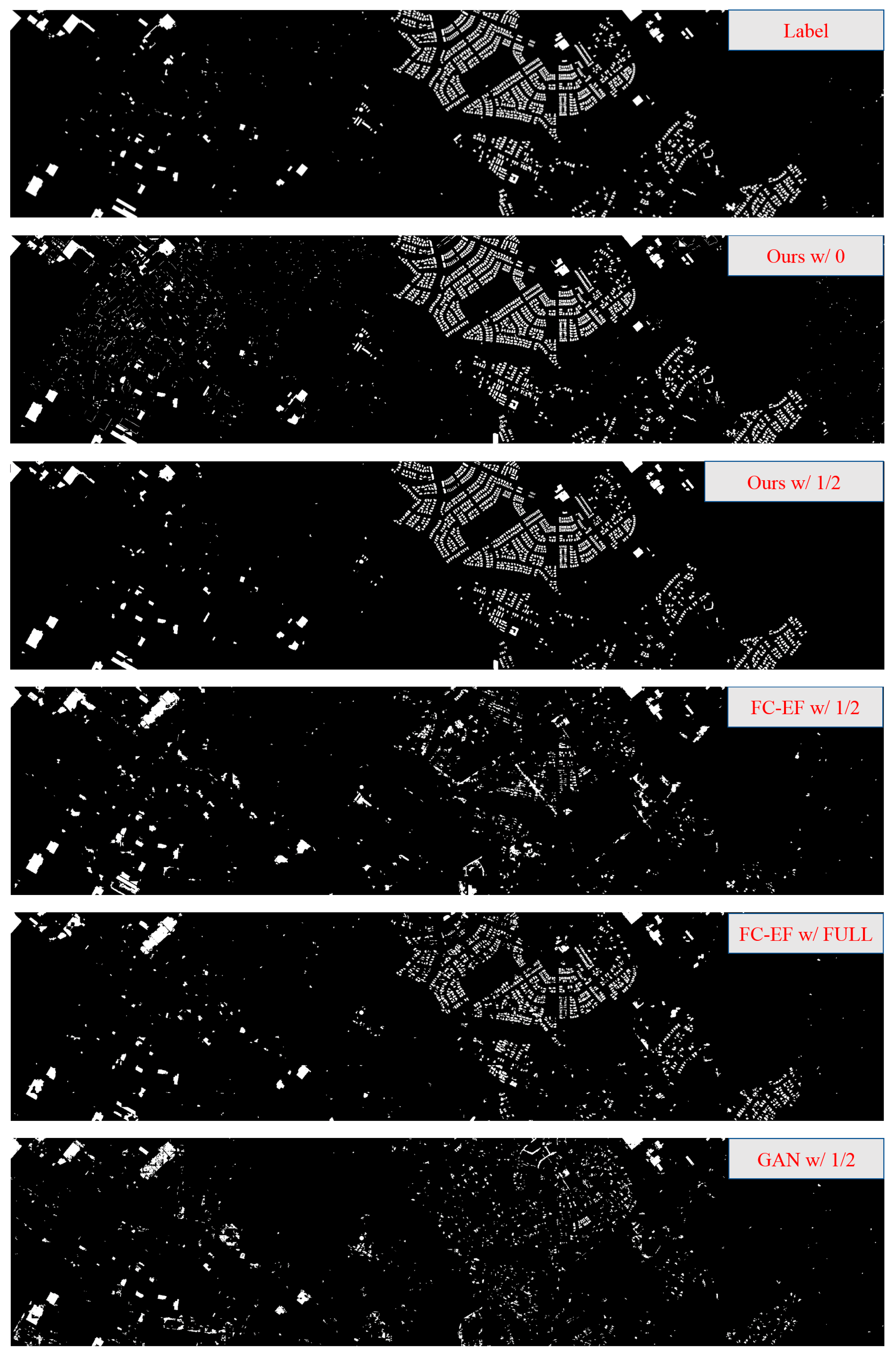
3.3. Building Change Detection Results
4. Discussion
5. Conclusions
Author Contributions
Funding
Conflicts of Interest
References
- Singh, A. Review Article Digital change detection techniques using remotely-sensed data. Inter. J. Remote Sens. 1989, 10, 989–1003. [Google Scholar] [CrossRef] [Green Version]
- Chen, G.; Hay, G.J.; Carvalho, L.M.; Wulder, M.A. Object-based change detection. Int. J. Remote Sens. 2012, 33, 4434–4457. [Google Scholar] [CrossRef]
- Coops, N.C.; Wulder, M.A.; White, J.C. Identifying and describing forest disturbance and spatial pattern: data selection issues and methodological implications. In Forest Disturbance and Spatial Pattern: Remote Sensing and GIS Approaches; CRC Press (Taylor and Francis): Boca Raton, FL, USA, 2006; pp. 33–60. [Google Scholar]
- Lunetta, R.S.; Johnson, D.M.; Lyon, J.G.; Crotwell, J. Impacts of imagery temporal frequency on land-cover change detection monitoring. Remote. Sens. Environ. 2004, 89, 444–454. [Google Scholar] [CrossRef]
- Shalaby, A.; Tateishi, R. Remote sensing and GIS for mapping and monitoring land cover and land-use changes in the Northwestern coastal zone of Egypt. Appl. Geogr. 2007, 27, 28–41. [Google Scholar] [CrossRef]
- Peiman, R. Pre-classification and post-classification change-detection techniques to monitor land-cover and land-use change using multi-temporal Landsat imagery: A case study on Pisa Province in Italy. Int. J. Remote. Sens. 2011, 32, 4365–4381. [Google Scholar] [CrossRef]
- Ochoa-Gaona, S.; González-Espinosa, M. Land use and deforestation in the highlands of Chiapas, Mexico. Appl. Geogr. 2000, 20, 17–42. [Google Scholar] [CrossRef]
- Green, K.; Kempka, D.; Lackey, L. Using remote sensing to detect and monitor land-cover and land-use change. Photogramm. Eng. Remote Sens. 1994, 60, 331–337. [Google Scholar]
- Torres-Vera, M.A.; Prol-Ledesma, R.M.; García-López, D. Three decades of land use variations in Mexico City. Int. J. Remote. Sens. 2008, 30, 117–138. [Google Scholar] [CrossRef]
- Jenson, J. Detecting residential land use development at the urban fringe. Photogramm. Eng. Remote Sens. 1982, 48, 629–643. [Google Scholar]
- Deng, J.S.; Wang, K.; Deng, Y.H.; Qi, G.J. PCA-based land-use change detection and analysis using multitemporal and multisensor satellite data. Int. J. Remote. Sens. 2008, 29, 4823–4838. [Google Scholar]
- Koltunov, A.; Ustin, S. Early fire detection using non-linear multitemporal prediction of thermal imagery. Remote. Sens. Environ. 2007, 110, 18–28. [Google Scholar] [CrossRef]
- Coops, N.C.; Gillanders, S.N.; Wulder, M.A.; Gergel, S.E.; Nelson, T.; Goodwin, N.R. Assessing changes in forest fragmentation following infestation using time series Landsat imagery. For. Ecol. Manag. 2010, 259, 2355–2365. [Google Scholar] [CrossRef]
- Hame, T.; Heiler, I.; San Miguel-Ayanz, J. An unsupervised change detection and recognition system for forestry. Int. J. Remote. Sens. 2010, 19, 1079–1099. [Google Scholar] [CrossRef]
- Wulder, M.A.; Butson, C.R.; White, J.C. Cross-sensor change detection over a forested landscape: Options to enable continuity of medium spatial resolution measures. Remote. Sens. Environ. 2008, 112, 796–809. [Google Scholar] [CrossRef]
- Deer, P. Digital Change Detection Techniques in Remote Sensing; Defence Science and Technology Organization: Canberra, Australia, 1995. [Google Scholar]
- Jenson, J. Urban/suburban land use analysis. In Manual of Remote Sensing; American Society of Photogrammetry, 1983; pp. 1571–1666. Available online: https://ci.nii.ac.jp/naid/10003189509/ (accessed on 3 May 2019).
- Hussain, M.; Chen, D.; Cheng, A.; Wei, H.; Stanley, D. Change detection from remotely sensed images: From pixel-based to object-based approaches. ISPRS J. Photogramm. Remote. Sens. 2013, 80, 91–106. [Google Scholar] [CrossRef]
- Lu, D.; Mausel, P.; Brondizio, E.; Moran, E. Change detection techniques. Int. J. Remote Sens. 2004, 25, 2365–2401. [Google Scholar] [CrossRef]
- Chen, X.; Vierling, L.; Deering, D. A simple and effective radiometric correction method to improve landscape change detection across sensors and across time. Remote. Sens. Environ. 2005, 98, 63–79. [Google Scholar] [CrossRef]
- Du, Y.; Teillet, P.M.; Cihlar, J. Radiometric normalization of multitemporal high-resolution satellite images with quality control for land cover change detection. Remote. Sens. Environ. 2002, 82, 123–134. [Google Scholar] [CrossRef]
- Huang, X.; Zhang, L.; Zhu, T. Building change detection from multitemporal high-resolution remotely sensed images based on a morphological building index. IEEE J. Sel. Top. Appl. Earth Obs. Remote Sens. 2014, 7, 105–115. [Google Scholar] [CrossRef]
- Xiao, P.; Yuan, M.; Zhang, X.; Feng, X.; Guo, Y. Cosegmentation for Object-Based Building Change Detection From High-Resolution Remotely Sensed Images. IEEE Trans. Geosci. Remote. Sens. 2017, 55, 1587–1603. [Google Scholar] [CrossRef]
- Quarmby, N.A.; Cushnie, J.L. Monitoring urban land cover changes at the urban fringe from SPOT HRV imagery in south-east England. Int. J. Remote. Sens. 1989, 10, 953–963. [Google Scholar] [CrossRef]
- Howarth, P.J.; Wickware, G.M. Procedures for change detection using Landsat digital data. Int. J. Remote. Sens. 1981, 2, 277–291. [Google Scholar] [CrossRef]
- Ludeke, A.K.; Maggio, R.C.; Reid, L.M. An analysis of anthropogenic deforestation using logistic regression and GIS. J. Environ. Manag. 1990, 31, 247–259. [Google Scholar] [CrossRef]
- Lunetta, R.S.; Elvidge, C.D. Remote Sensing Change Detection; Taylor & Francis: Abingdon, UK, 1999; Volume 310. [Google Scholar]
- Richards, J. Thematic mapping from multitemporal image data using the principal components transformation. Remote. Sens. Environ. 1984, 16, 35–46. [Google Scholar] [CrossRef]
- Kauth, R.J.; Thomas, G. The tasselled cap--A graphic description of the spectral-temporal development of agricultural crops as seen by Landsat. In Proceedings of the LARS Symposia, West Lafayette, IN, USA, 29 June–1 July 1976; p. 159. [Google Scholar]
- Bovolo, F.; Bruzzone, L. A Theoretical Framework for Unsupervised Change Detection Based on Change Vector Analysis in the Polar Domain. IEEE Trans. Geosci. Remote. Sens. 2007, 45, 218–236. [Google Scholar] [CrossRef]
- Erener, A.; Düzgün, H.S. A methodology for land use change detection of high resolution pan images based on texture analysis. Ital. J. Remote. Sens. 2009, 41, 47–59. [Google Scholar] [CrossRef]
- Tomowski, D.; Ehlers, M.; Klonus, S. Colour and texture based change detection for urban disaster analysis. In Proceedings of the 2011 Joint Urban Remote Sensing Event (JURSE 2011), Munich, Germany, 11–13 April 2011; pp. 329–332. [Google Scholar]
- Im, J.; Jensen, J.R. A change detection model based on neighborhood correlation image analysis and decision tree classification. Remote. Sens. Environ. 2005, 99, 326–340. [Google Scholar] [CrossRef]
- Bouziani, M.; Goïta, K.; He, D.-C. Automatic change detection of buildings in urban environment from very high spatial resolution images using existing geodatabase and prior knowledge. ISPRS J. Photogramm. Remote. Sens. 2010, 65, 143–153. [Google Scholar] [CrossRef]
- Yuan, F.; Sawaya, K.E.; Loeffelholz, B.C.; Bauer, M.E. Land cover classification and change analysis of the Twin Cities (Minnesota) Metropolitan Area by multitemporal Landsat remote sensing. Remote. Sens. Environ. 2005, 98, 317–328. [Google Scholar] [CrossRef]
- Serpico, S.B.; Moser, G. Weight Parameter Optimization by the Ho–Kashyap Algorithm in MRF Models for Supervised Image Classification. IEEE Trans. Geosci. Remote. Sens. 2006, 44, 3695–3705. [Google Scholar] [CrossRef]
- Wiemker, R. An iterative spectral-spatial Bayesian labeling approach for unsupervised robust change detection on remotely sensed multispectral imagery. In Proceedings of the Transactions on Rough Sets VII, Kiel, Germany, 10–12 September 1997; Volume 1296, pp. 263–270. [Google Scholar]
- Melgani, F.; Bazi, Y. Markovian Fusion Approach to Robust Unsupervised Change Detection in Remotely Sensed Imagery. IEEE Geosci. Remote. Sens. Lett. 2006, 3, 457–461. [Google Scholar] [CrossRef]
- Pijanowski, B.C.; Pithadia, S.; Shellito, B.A.; Alexandridis, K.; Alexandridis, K. Calibrating a neural network-based urban change model for two metropolitan areas of the Upper Midwest of the United States. Int. J. Geogr. Inf. Sci. 2005, 19, 197–215. [Google Scholar] [CrossRef]
- Liu, X.; Lathrop, R.G. Urban change detection based on an artificial neural network. Int. J. Remote. Sens. 2002, 23, 2513–2518. [Google Scholar] [CrossRef]
- Nemmour, H.; Chibani, Y. Multiple support vector machines for land cover change detection: An application for mapping urban extensions. ISPRS J. Photogramm. Remote. Sens. 2006, 61, 125–133. [Google Scholar] [CrossRef]
- Huang, C.; Song, K.; Kim, S.; Townshend, J.R.; Davis, P.; Masek, J.G.; Goward, S.N. Use of a dark object concept and support vector machines to automate forest cover change analysis. Remote. Sens. Environ. 2008, 112, 970–985. [Google Scholar] [CrossRef]
- Hall, O.; Hay, G.J. A Multiscale Object-Specific Approach to Digital Change Detection. Int. J. Appl. Earth Obs. Geoinf. 2003, 4, 311–327. [Google Scholar] [CrossRef]
- Lefebvre, A.; Corpetti, T.; Hubert-Moy, L. Object-Oriented Approach and Texture Analysis for Change Detection in Very High Resolution Images. In Proceedings of the IGARSS 2008 - 2008 IEEE International Geoscience and Remote Sensing Symposium, Boston, MA, USA, 7–11 July 2008. [Google Scholar]
- Fisher, P. The pixel: a snare and a delusion. Int. J. Remote Sens. 1997, 18, 679–685. [Google Scholar] [CrossRef]
- De Chant, T.; Kelly, N.M. Individual Object Change Detection for Monitoring the Impact of a Forest Pathogen on a Hardwood Forest. Photogramm. Eng. Remote. Sens. 2009, 75, 1005–1013. [Google Scholar] [CrossRef] [Green Version]
- Conchedda, G.; Durieux, L.; Mayaux, P. An object-based method for mapping and change analysis in mangrove ecosystems. ISPRS J. Photogramm. Remote. Sens. 2008, 63, 578–589. [Google Scholar] [CrossRef]
- Du, S.; Zhang, Y.; Qin, R.; Yang, Z.; Zou, Z.; Tang, Y.; Fan, C. Building Change Detection Using Old Aerial Images and New LiDAR Data. Remote. Sens. 2016, 8, 1030. [Google Scholar] [CrossRef]
- Liu, H.; Yang, M.; Chen, J.; Hou, J.; Deng, M. Line-Constrained Shape Feature for Building Change Detection in VHR Remote Sensing Imagery. ISPRS Int. J. Geo-Inf. 2018, 7, 410. [Google Scholar] [CrossRef]
- Gong, M.; Niu, X.; Zhang, P.; Li, Z. Generative Adversarial Networks for Change Detection in Multispectral Imagery. IEEE Geosci. Remote. Sens. Lett. 2017, 14, 2310–2314. [Google Scholar] [CrossRef]
- Zhang, P.; Gong, M.; Su, L.; Liu, J.; Li, Z. Change detection based on deep feature representation and mapping transformation for multi-spatial-resolution remote sensing images. ISPRS J. Photogramm. Remote. Sens. 2016, 116, 24–41. [Google Scholar] [CrossRef]
- Mou, L.; Bruzzone, L.; Zhu, X.X. Learning Spectral-Spatial-Temporal Features via a Recurrent Convolutional Neural Network for Change Detection in Multispectral Imagery. IEEE Trans. Geosci. Remote. Sens. 2019, 57, 924–935. [Google Scholar] [CrossRef]
- Gong, M.; Zhan, T.; Zhang, P.; Miao, Q. Superpixel-Based Difference Representation Learning for Change Detection in Multispectral Remote Sensing Images. IEEE Trans. Geosci. Remote. Sens. 2017, 55, 1–16. [Google Scholar] [CrossRef]
- Wang, Q.; Yuan, Z.; Du, Q.; Li, X. GETNET: A General End-to-End 2-D CNN Framework for Hyperspectral Image Change Detection. IEEE Trans. Geosci. Remote. Sens. 2019, 57, 3–13. [Google Scholar] [CrossRef]
- Gong, M.; Zhao, J.; Liu, J.; Miao, Q.; Jiao, L. Change Detection in Synthetic Aperture Radar Images Based on Deep Neural Networks. IEEE Trans. Neural Netw. Learn. Syst. 2016, 27, 125–138. [Google Scholar] [CrossRef]
- Khan, S.H.; He, X.; Porikli, F.; Bennamoun, M. Forest Change Detection in Incomplete Satellite Images With Deep Neural Networks. IEEE Trans. Geosci. Remote. Sens. 2017, 55, 5407–5423. [Google Scholar] [CrossRef]
- Ding, A.; Zhang, Q.; Zhou, X.; Dai, B. Automatic recognition of landslide based on CNN and texture change detection. In Proceedings of the 2016 31st Youth Academic Annual Conference of Chinese Association of Automation (YAC), Wuhan, China, 11–13 November 2016; pp. 444–448. [Google Scholar]
- Krizhevsky, A.; Sutskever, I.; Hinton, G.E. Imagenet classification with deep convolutional neural networks. In Proceedings of the Advances in Neural Information Processing Systems, Lake Tahoe, NV, USA, 3–8 December 2012; pp. 1097–1105. [Google Scholar]
- Hinton, G.E.; Osindero, S.; Teh, Y.-W. A Fast Learning Algorithm for Deep Belief Nets. Neural Comput. 2006, 18, 1527–1554. [Google Scholar] [CrossRef]
- Zhang, F.; Du, B.; Zhang, L. Saliency-Guided Unsupervised Feature Learning for Scene Classification. IEEE Trans. Geosci. Remote. Sens. 2015, 53, 2175–2184. [Google Scholar] [CrossRef]
- Goodfellow, I.; Pouget-Abadie, J.; Mirza, M.; Xu, B.; Warde-Farley, D.; Ozair, S.; Courville, A.; Bengio, Y. Generative adversarial nets. In Proceedings of the Advances in Neural Information Processing Systems, Montréal, QC, Canada, 8–13 December 2014; pp. 2672–2680. [Google Scholar]
- Daudt, R.C.; Saux, B.L.; Boulch, A. Fully Convolutional Siamese Networks for Change Detection. In Proceedings of the 2018 25th IEEE International Conference on Image Processing (ICIP), Athens, Greece, 7–10 October 2018; pp. 4063–4067. [Google Scholar]
- Nemoto, K.; Imaizumi, T.; Hikosaka, S.; Hamaguchi, R.; Sato, M.; Fujita, A. Building change detection via a combination of CNNs using only RGB aerial imageries. Remote Sens. Tech. Appl. Urban Environ. 2017, 10431, 23. [Google Scholar]
- Zhang, Z.; Vosselman, G.; Gerke, M.; Tuia, D.; Yang, M.Y. Change Detection between Multimodal Remote Sensing Data Using Siamese CNN. arXiv 2018, arXiv:1807.09562. [Google Scholar]
- El Amin, A.M.; Liu, Q.; Wang, Y. Zoom out CNNs features for optical remote sensing change detection. In Proceedings of the 2017 2nd International Conference on Image, Vision and Computing (ICIVC), Chengdu, China, 2–4 June 2017; pp. 812–817. [Google Scholar]
- Ji, S.; Wei, S.; Lu, M. Fully Convolutional Networks for Multisource Building Extraction From an Open Aerial and Satellite Imagery Data Set. IEEE Trans. Geosci. Remote. Sens. 2019, 57, 574–586. [Google Scholar] [CrossRef]
- He, K.; Gkioxari, G.; Dollár, P.; Girshick, R. Mask R-CNN. In Proceedings of the 2017 IEEE International Conference on Computer Vision (ICCV), Venice, Italy, 22–29 October 2017; pp. 2980–2988. [Google Scholar]
- Ronneberger, O.; Fischer, P.; Brox, T. U-Net: Convolutional Networks for Biomedical Image Segmentation. In Lecture Notes in Computer Science; Springer Nature: Switzerland, 2015; Volume 9351, pp. 234–241. Available online: https://link.springer.com/chapter/10.1007/978-3-319-24574-4_28 (accessed on 3 May 2019).
- Ren, S.; He, K.; Girshick, R.; Sun, J. Faster R-CNN: Towards Real-Time Object Detection with Region Proposal Networks. IEEE Trans. Pattern Anal. Mach. Intell. 2017, 39, 1137–1149. [Google Scholar] [CrossRef] [Green Version]
- Lebedev, M.A.; Vizilter, Y.V.; Vygolov, O.V.; Knyaz, V.A.; Rubis, A.Y. Change detection in remote sensing images using conditional adversarial networks. ISPRS - Int. Arch. Photogramm. Remote. Sens. Spat. Inf. Sci. 2018, XLII-2, 565–571. [Google Scholar] [CrossRef]
- Chen, L.-C.; Zhu, Y.; Papandreou, G.; Schroff, F.; Adam, H. Encoder-Decoder with Atrous Separable Convolution for Semantic Image Segmentation. In Proceedings of the Topics in Artificial Intelligence, Munich, Germany, 8–14 September 2018; pp. 833–851. [Google Scholar]
- Lin, T.-Y.; Maire, M.; Belongie, S.; Hays, J.; Perona, P.; Ramanan, D.; Dollár, P.; Zitnick, C.L. Microsoft COCO: Common Objects in Context. In Proceedings of the Transactions on Rough Sets VII, Zurich, Switzerland, 6–12 September 2014; Volume 8693, pp. 740–755. [Google Scholar]
- Chatzis, V.; Krinidis, S. A Robust Fuzzy Local Information C-Means Clustering Algorithm. IEEE Trans. Image Process. 2010, 19, 1328–1337. [Google Scholar]
- Dalal, N. Finding People in Images and Videos; Institut National Polytechnique de Grenoble-INPG: Grenoble, France, 2006. [Google Scholar]
- OpenStreetMap. Available online: https://www.openstreetmap.org (accessed on 30 April 2019).


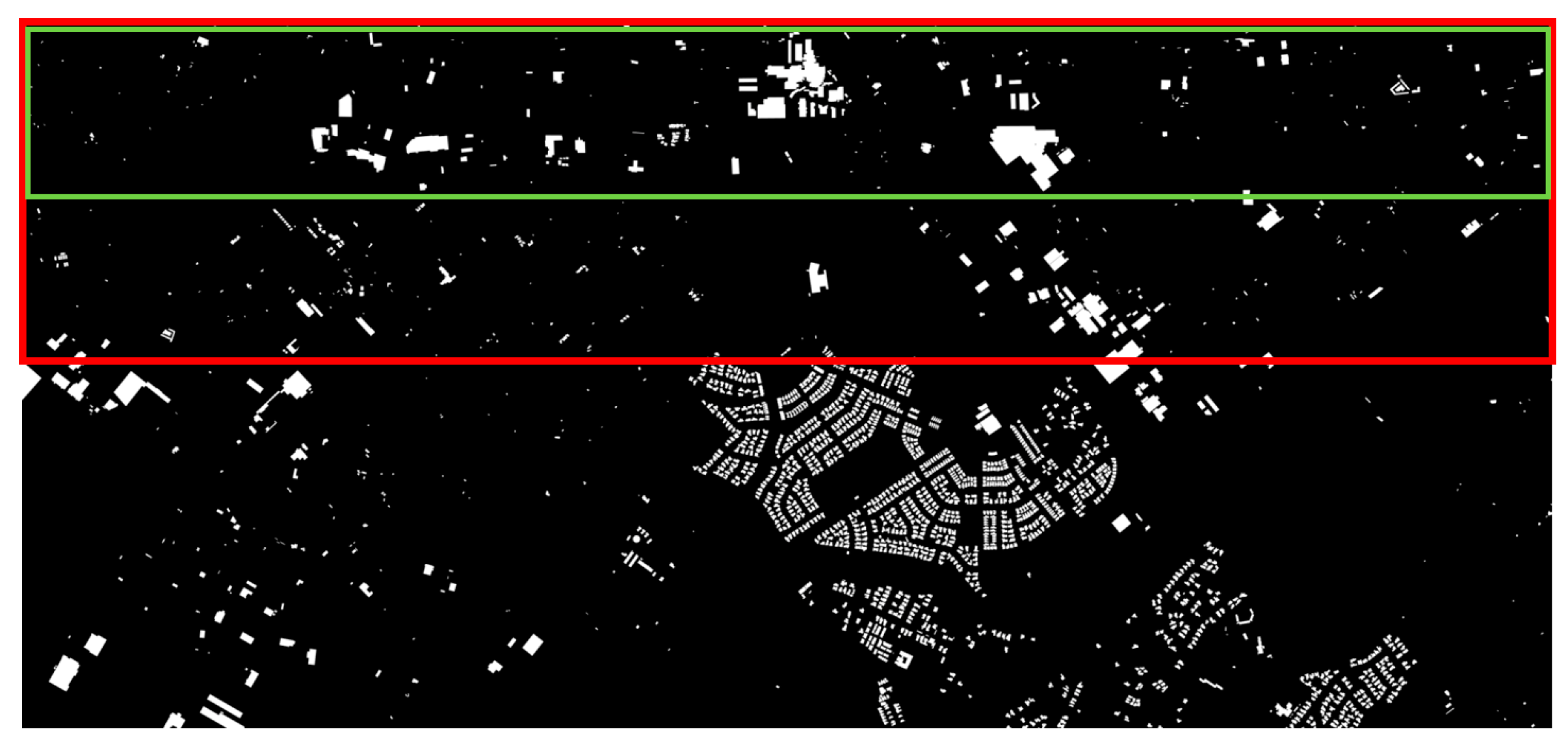
| Datasets | GSD (m) | Area (km2) | Tiles | Pixels | Building Number | Box Color (Figure 6) |
|---|---|---|---|---|---|---|
| SC-2016 | 0.2 | 57.744 | 5400 | 512 × 512 | 67,190 | Yellow |
| SC-2011 | 0.2 | 22.035 | 2065 | 512 × 512 | 11,495 | Green |
| TA-2016 | 0.2 | 19.964 | 1827 | 512 × 512 | 11,595 | Red |
| TA-2011 | 0.2 | 19.964 | 1827 | 512 × 512 | 9588 | Red |
| SI-2016 | 0.2 | 20.294 | 1892 | 512 × 512 | 21,876 | Blue |
| Dataset | Method | Objected-Based | Pixel-Based | |||||||
|---|---|---|---|---|---|---|---|---|---|---|
| AP | Precision | Recall | TP+FP | TP | TP+FN | IoU | Precision | Recall | ||
| TA-2011 | Mask R-CNN | 0.833 | 0.892 | 0.930 | 9993 | 8916 | 9588 | 0.867 | 0.943 | 0.915 |
| MS-FCN | 0.773 | 0.922 | 0.837 | 8702 | 8022 | 9588 | 0.869 | 0.934 | 0.925 | |
| TA-2016 | Mask R-CNN | 0.858 | 0.922 | 0.929 | 11,684 | 10,768 | 11,595 | 0.897 | 0.956 | 0.936 |
| MS-FCN | 0.857 | 0.939 | 0.911 | 11,243 | 10,560 | 11,595 | 0.920 | 0.960 | 0.957 | |
| Dataset | Extraction Method | Objected-Based | Pixel-Based | |||||||
|---|---|---|---|---|---|---|---|---|---|---|
| AP | Precision | Recall | TP+FP | TP | TP + FN | IoU | Precision | Recall | ||
| simulated | Mask R-CNN | 0.630 | 0.644 | 0.943 | 2511 | 1618 | 1715 | 0.798 | 0.856 | 0.922 |
| MS-FCN | 0.609 | 0.659 | 0.896 | 2332 | 1537 | 1715 | 0.798 | 0.839 | 0.943 | |
| Half | Mask R-CNN | 0.806 | 0.928 | 0.857 | 1584 | 1470 | 1715 | 0.773 | 0.952 | 0.804 |
| MS-FCN | 0.793 | 0.881 | 0.880 | 1714 | 1510 | 1715 | 0.843 | 0.912 | 0.918 | |
| FC-EF [62] | 0.027 | 0.200 | 0.114 | 980 | 196 | 1715 | 0.261 | 0.516 | 0.346 | |
| GAN [70] | 0.023 | 0.135 | 0.127 | 1616 | 218 | 1715 | 0.232 | 0.538 | 0.290 | |
| Full | Mask R-CNN | 0.814 | 0.910 | 0.883 | 1663 | 1514 | 1715 | 0.837 | 0.931 | 0.892 |
| MS-FCN | 0.796 | 0.891 | 0.872 | 1679 | 1496 | 1715 | 0.830 | 0.938 | 0.878 | |
| FC-EF [62] | 0.254 | 0.519 | 0.462 | 1525 | 792 | 1715 | 0.502 | 0.767 | 0.593 | |
| GAN [70] | / | / | / | / | / | / | / | / | / | |
| Method | AP | Precision | Recall |
|---|---|---|---|
| Difference | 0.010 | 0.010 | 0.872 |
| Distance & IoU 1 | 0.290 | 0.345 | 0.839 |
| Distance & IoU 2 | 0.290 | 0.343 | 0.844 |
| Erode & dilate | 0.388 | 0.489 | 0.793 |
| Erode & intersect | 0.450 | 0.540 | 0.832 |
| Our network | 0.630 | 0.644 | 0.943 |
| Method | IoU | Precision | Recall |
|---|---|---|---|
| Differencing [24] | 0.667 | 0.709 | 0.918 |
| ratioing [25] | 0.667 | 0.709 | 0.918 |
| FLICM [73] | 0.678 | 0.723 | 0.917 |
| Our network | 0.798 | 0.856 | 0.922 |
© 2019 by the authors. Licensee MDPI, Basel, Switzerland. This article is an open access article distributed under the terms and conditions of the Creative Commons Attribution (CC BY) license (http://creativecommons.org/licenses/by/4.0/).
Share and Cite
Ji, S.; Shen, Y.; Lu, M.; Zhang, Y. Building Instance Change Detection from Large-Scale Aerial Images using Convolutional Neural Networks and Simulated Samples. Remote Sens. 2019, 11, 1343. https://doi.org/10.3390/rs11111343
Ji S, Shen Y, Lu M, Zhang Y. Building Instance Change Detection from Large-Scale Aerial Images using Convolutional Neural Networks and Simulated Samples. Remote Sensing. 2019; 11(11):1343. https://doi.org/10.3390/rs11111343
Chicago/Turabian StyleJi, Shunping, Yanyun Shen, Meng Lu, and Yongjun Zhang. 2019. "Building Instance Change Detection from Large-Scale Aerial Images using Convolutional Neural Networks and Simulated Samples" Remote Sensing 11, no. 11: 1343. https://doi.org/10.3390/rs11111343
APA StyleJi, S., Shen, Y., Lu, M., & Zhang, Y. (2019). Building Instance Change Detection from Large-Scale Aerial Images using Convolutional Neural Networks and Simulated Samples. Remote Sensing, 11(11), 1343. https://doi.org/10.3390/rs11111343