Discovering the Representative Subset with Low Redundancy for Hyperspectral Feature Selection

Abstract

In this paper, a novel unsupervised band selection (BS) criterion based on maximizing representativeness and minimizing redundancy (MRMR) is proposed for selecting a set of informative bands to represent the whole hyperspectral image cube. The new selection criterion is denoted as the MRMR selection criterion and the associated BS method is denoted as the MRMR method. The MRMR selection criterion can evaluate the band subset’s representativeness and redundancy simultaneously. For one band subset, its representativeness is estimated by using orthogonal projection (OP) and its redundancy is measured by the average of the Pearson correlation coefficients among the bands in this subset. To find the satisfactory subset, an effective evolutionary algorithm, i.e., the immune clone selection (ICS) algorithm, is applied as the subset searching strategy. Moreover, we further introduce two effective tricks to simplify the computation of the representativeness metric, thus the computational complexity of the proposed method is reduced significantly. Experimental results on different real-world datasets demonstrate that the proposed method is very effective and its selected bands can obtain good classification performances in practice.

1. Introduction

Hyperspectral images contain large amounts of bands, which brings several problems, such as the heavy computational burden and storage cost. In addition, there is high correlation among the hyperspectral bands due to the high resolution of spectrum, using all the bands is unnecessary. Therefore, it is necessary to perform dimensionality reduction (DR) for processing the hyperspectral data effectively. The commonly used DR techniques include feature extraction and band selection (i.e., feature selection). Feature extraction reduces the feature space by extracting a few new features from the original features through some function mapping, this kind of methods include principal component analysis (PCA) [1,2], nonnegative matrix factorization (NMF) [3], and so on [4,5,6,7]. Different from feature extraction, band selection directly selects a subset of features from the original ones. For hyperspectral imagery, band selection (BS) is preferable because the selected bands still have the physical meaning and preserve the relevant original information in the data. BS methods can be broadly split into the supervised and unsupervised methods in terms of the prior knowledge availability. Supervised BS methods try to find the most informative bands with respect to the available prior knowledge [8,9], whereas unsupervised methods do not use any object information [10,11]. Because the prior knowledge is often unavailable in practice, developing unsupervised BS techniques is necessary.

Many unsupervised band selection methods have been proposed in these years. Some of them use different information criteria to measure the importance of hyperspectral bands, then all the bands are sorted and several top ranked bands would be selected. These kind of methods include information divergence BS (IDBS) [10], linearly constraint minimum variance (LCMV) [10], constrained band selection (CBS) [10], mutual information [12], maximum-variance principal component analysis (MVPCA) [13] and so on [14]. Other band selection methods take bands’ correlation into consideration. For instance, the maximum ellipsoid volume (MEV) based methods [15,16,17,18] measure the importance of band subsets by calculating the ellipsoid volume of band subsets, and it has been proved that this kind of methods can well consider the correlation among bands [19]. Recently, some BS methods based on orthogonal projection (OP) are proposed [19,20,21,22], these methods use OP to select the bands with low redundancy and they have shown good performances in practice. Additionally, many BS methods based on advanced machine learning algorithms are also proposed, these methods include the clustering-based methods [23,24,25,26,27], manifold ranking (MR) [28], sparsity based BS methods [29,30], graph theory based BS [11] and so on.

Through analyzing the selection criteria of these BS methods, it can be found that, generally, band-ranking based methods mainly consider bands’ information but neglect the correlation among selected bands [10,21]; although the correlation-based methods pay sufficient attention on band correlation, their selected bands are not always highly representative and thus the classification performances are not very satisfactory [11,20,21]; clustering-based methods and some other advanced methods may take into account information and correlation implicitly, but their computational burden is usually heavy and there is still a large room for improvement in the selection criteria [21,28]. Therefore, we aim to design a new BS method which explicitly considers the bands’ information and redundancy simultaneously.

In this paper, we proposed a novel BS selection criterion based on maximizing representativeness and minimizing redundancy, which is denoted as the MRMR selection criterion. Combine the MRMR selection criterion with the immune clone selection (ICS) [31], a new method named the MRMR BS method is obtained. The MRMR selection criterion is based on orthogonal projection (OP) [19] and it provides a novel perspective for evaluating the importance of band subsets; The MRMR selection criterion consists of two metrics, i.e., the representativeness metric and the redundancy metric. The orthogonal projection is used to evaluate the representativeness of a band subset, and the average of the Pearson correlation coefficients among the bands in the band subset is used to measure the redundancy of this band set. By combining these two metrics properly, the MRMR selection criterion can evaluate the importance of each candidate band subset. After the selection criterion has been determined, the BS task is reduced to be a subset searching problem, namely, we need to traverse all the candidate band subsets to find the satisfactory one. Since exhaustive searching strategy is impractical, we have to apply a suboptimal group searching strategy. In this paper, a simple but effective evolutionary searching algorithm, i.e., the immune clone selection (ICS) algorithm, is applied as the subset searching strategy. ICS ensures that the BS algorithm can obtain the desired band subset in a reasonable time. Furthermore, to ease the huge computation burden caused by orthogonal projection, two efficient tricks are introduced to simplify the computation of representativeness metric, and these tricks may be also helpful for reducing the computational complexity of other similar OP-based methods. The major contribution of this paper can be summarized as follows: (1) A new perspective, that is, the selected features should not only well represent the whole feature set but also have low redundancy among themselves, is provided for measuring the importance of feature subset in unsupervised feature selection. (2) Based on the above basic idea for designing selection criteria, the OP and mean correlation coefficient are respectively used for evaluating the representativeness and redundancy of feature subsets, and the MRMR selection criterion is proposed. (3) Two ways are introduced to accelerate the proposed method, and these tricks may be also helpful for reducing the computational complexity of other similar methods.

The remainder of this paper is organized as follows: Section 2 introduces some related works associated with the proposed method, and Section 3 specifically explains the proposed method. Section 4 presents experiments on different real-world hyperspectral images. Finally, Section 5 gives some concluding remarks.

2. Related Works

The proposed MRMR method aims to find the band subset that can best represent the whole image dataset. Some similar methods can be found in [10], in which the linearly constraint minimum variance based methods (LCMV) are proposed. The LCMV-based methods design a finite impulse response (FIR) filter for bands, and by minimizing the averaged least squares filter output, the band selection is transferred to an optimization problem that is similar to the constrained energy minimization (CEM) [32]. LCMV can find the bands that best represent the whole image, but it tackles each band individually and does not consider the band redundancy among the selected bands, so the bands obtained by this kind of methods may be highly correlated with each other. In practice, the high correlation among selected features often deteriorates the performances of classification, so a good band selection method should consider band correlation for obtaining good classification performances.

For the MRMR method, we use OP to measure the representativeness of a subset relative to the whole image cube. Namely, for a candidate band subset, we orthogonally project each remaining band (all the bands excluded in this subset) to the vector space spanned by the bands of the subset, then the sum of all the remaining bands’s distances to their OPs can reflect the representativeness of this band subset. Some methods based on similar processes have been proposed, for instance, the orthogonal-projection-based BS method (OPBS) [19], the OSP based BS method (OSP-BSVD) [21], and the volume-gradient-based BS method (VGBS) [20]; all these methods can be considered as the BS methods based on OP. OPBS and OSP-BSVD have almost the same selection criterion, but they are derived independently from different perspectives. Since OPBS and OSP-BSVD are quite similar, for convenience, we only compare the OPBS method with the proposed method in the following. The OPBS method applies sequential forward search (SFS) [33] as the searching strategy, so it selects one band for each time. For the OPBS method, at each round of lookup, the band that has the maximum OP onto the orthogonal complement of the vector space spanned by the currently selected bands would be regarded as the target band and added into the selected band set [19]. VGBS is similar to OPBS, but it removes one band from the original band set iteratively, until the desired number of bands retain [20]. These similar OP-based methods mainly consider the redundancy of bands but pay insufficiently attention on the representativeness of bands, so the selected bands obtained by these methods usually have low redundancy but may not represent the whole dataset well [19,20].

The major differences between the proposed MRMR method and these similar methods could be summarized as follows:

(1)

When compared with the the LCMV-based methods; although both the LCMV-based methods and the MRMR method evaluate the representativeness of bands, their explicit selection criteria are totally different. The LCMV-based methods measure one band’s representativeness relative to the whole dataset by using a finite impulse response (FIR) filter [10]. The MRMR method evaluates the representativeness of a band subset relative to the remaining bands by using OP. Moreover, LCMV cannot consider redundancy among selected bands [10,19], but the MRMR method can achieve it.

(2)

When compared with the existing OP-based methods like OPBS, OSP-BSVD and VGBS; although both these similar methods and the MRMR method use OP to measure the relationship among bands, their objectives are totally different. For the OPBS, OSP-BSVD and VGBS methods, OP is used to evaluate the redundancy or the dissimilarity between a candidate band and the currently selected bands [19,20,21]; while for the MRMR method, OP is used to measure the representativeness of a band subset relative to the remaining unselected bands. The existing OP-based mainly consider the redundancy among selected bands but do not pay sufficient attention on the selected bands’ representativeness [19], in contrast, the MRMR method can well consider both the redundancy and the representativeness of the selected band subset.

(3)

Finally, all the LCMV, OPBS, OSP-BSVD and VGBS methods are point-wise band selection methods, namely, the desired bands are obtained individually [10,19,20,21]; whereas the MRMR method is a group-wise method, in which the desired bands are obtained simultaneously. Because the selected bands actually works together in the applications like pixel classification, the effect of the selected bands should be considered jointly. The group-wise methods are usually more effective than the point-wise methods, since the group searching strategy is more suitable for evaluating the joint effect of multiple bands.

3. The Proposed Method

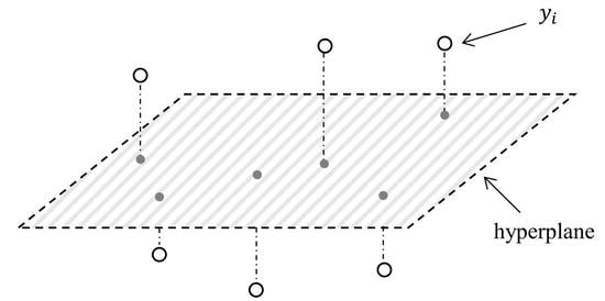
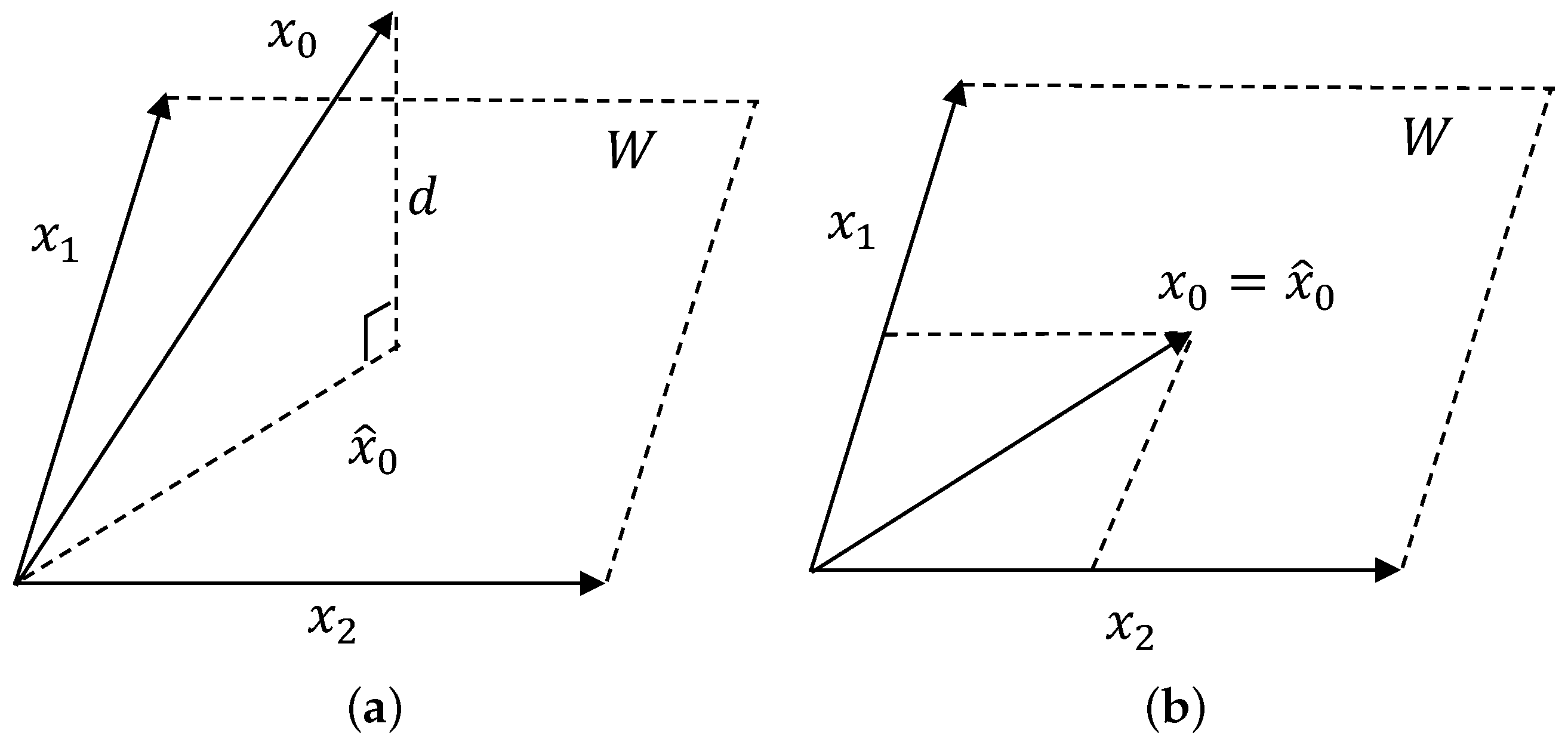
3.1. Background of OP

The selection criterion of the MRMR method is associated with the vector space. In linear algebra, a vector space is defined as a set that is closed under finite vector addition and scalar multiplication [34]. Suppose that there is a set of column vectors which is denoted as $\mathit{A}=\left[{\mathit{x}}_{\mathbf{1}},{\mathit{x}}_{\mathbf{2}},\cdots ,{\mathit{x}}_{\mathit{m}}\right]\in {\mathbb{R}}^{N\times m}$, where N and m represent the numbers of elements and vectors, respectively, then the vector space spanned by all the column vectors of $\mathit{A}$ can be denoted as follows:

$$W=Span\left\{\mathit{A}\right\}=\{\mathit{x}:\mathit{x}=\sum _{i=1}^m{a}_i·{\mathit{x}}_{\mathit{i}},a_i\in \mathbb{R}\}$$

(1)

where $a_i$ could be any scalar. Assume that there is another column vector ${\mathit{x}}_{\mathbf{0}}$, if we want to evaluate its relationship with the vector set $\mathit{A}$, we can compute the distance of ${\mathit{x}}_{\mathbf{0}}$ to the vector set $\mathit{A}$. The distance can be obtained by orthogonally projecting the vector ${\mathit{x}}_{\mathbf{0}}$ onto the vector space W. In linear algebra, W is also a linear subspace (or a linear manifold) of the vector space spanned by the vector set $\left\{{\mathit{x}}_{\mathbf{0}},{\mathit{x}}_{\mathbf{1}},{\mathit{x}}_{\mathbf{2}},\cdots ,{\mathit{x}}_{\mathit{m}}\right\}$ (note that this set includes ${\mathit{x}}_{\mathbf{0}}$), so W can be considered as a hyperplane relative to the latter [34]. The orthogonal projection of ${\mathit{x}}_{\mathbf{0}}$ onto the hyperplane W can be computed by:

$$\mathit{P}=\mathit{A}{\left({\mathit{A}}^T\mathit{A}\right)}^{-1}{\mathit{A}}^T$$

(2)

$${\widehat{\mathit{x}}}_{\mathbf{0}}=\mathit{P}·{\mathit{x}}_{\mathbf{0}}=\mathit{A}{\left({\mathit{A}}^T\mathit{A}\right)}^{-1}{\mathit{A}}^T·{\mathit{x}}_{\mathbf{0}}$$

(3)

where ${\widehat{\mathit{x}}}_{\mathbf{0}}$ is the orthogonal projection (OP) of ${\mathit{x}}_{\mathbf{0}}$ onto W, and $\mathit{P}$ is called the orthogonal projector. Then, the squared distance of ${\mathit{x}}_{\mathbf{0}}$ to the hyperplane W is

$$d=\parallel {\mathit{x}}_{\mathbf{0}}-{\widehat{\mathit{x}}}_{\mathbf{0}}{\parallel }^2$$

(4)

The squared distance d is also the squared norm of the orthogonal projection of ${\mathit{x}}_{\mathbf{0}}$ onto the orthogonal complement of W [19].

From the perspective of the linear regression, the orthogonal projection ${\widehat{\mathit{x}}}_{\mathbf{0}}$ is also the linear estimate or prediction of ${\mathit{x}}_{\mathbf{0}}$ using the vectors in $\mathit{A}$, and the distance d evaluates the prediction error [19]. More specifically, it is easy to find that the term ${\left({\mathit{A}}^T\mathit{A}\right)}^{-1}{\mathit{A}}^T{\mathit{x}}_{\mathbf{0}}$ in (3) is an $m\times 1$ vector and thus can be denoted as follows:

$$\mathit{\alpha }={[{\alpha }_1,{\alpha }_2,\cdots ,{\alpha }_m]}^T={\left({\mathit{A}}^T\mathit{A}\right)}^{-1}{\mathit{A}}^T{\mathit{x}}_{\mathbf{0}}$$

(5)

where ${\alpha }_i$ is a scalar, then the OP ${\widehat{\mathit{x}}}_{\mathbf{0}}$ is rewritten as

$${\widehat{\mathit{x}}}_{\mathbf{0}}=\mathit{A}\times \mathit{\alpha }=\sum _{i=1}^m{\alpha }_i·{\mathit{x}}_{\mathit{i}}$$

(6)

Obviously, the OP ${\widehat{\mathit{x}}}_{\mathbf{0}}$ is a linear combination of the vectors in $\mathit{A}$, and ${\left({\mathit{A}}^T\mathit{A}\right)}^{-1}{\mathit{A}}^T{\mathit{x}}_{\mathbf{0}}$ is the weight vector that determines how each vector affects the prediction. In fact, it can be proved that the term ${\left({\mathit{A}}^T\mathit{A}\right)}^{-1}{\mathit{A}}^T{\mathit{x}}_{\mathbf{0}}$ is exactly a least squared solution [19]. Therefore, the distance d is the linear prediction error and it reflects how difficult it is to use the vectors in $\mathit{A}$ to estimate the single vector ${\mathit{x}}_{\mathbf{0}}$. It is evident that, the smaller the distance d is, using the vectors in $\mathit{A}$ to linearly represent ${\mathit{x}}_{\mathbf{0}}$ is easier. For instance, Figure 1 shows an intuitive example in 3-D. In Figure 1a, the vector ${\mathit{x}}_{\mathbf{0}}$ cannot be totally linearly represented by the vectors ${\mathit{x}}_{\mathbf{1}}$ and ${\mathit{x}}_{\mathbf{2}}$, in other words, ${\mathit{x}}_{\mathbf{0}}$ does not belong to the vector space W, and correspondingly, the distance d does not equal zero; whereas in Figure 1b, the vector ${\mathit{x}}_{\mathbf{0}}$ belongs to the vector space W and thus it can be linearly represented by other vectors completely; in this case, the distance d equals zero. It can be found that, the distance of a vector to the hyperplane spanned by other vectors actually reflects the similarity between this single vector and a set of vectors. In band selection, if each band image is reshaped into a column vector, we can use OP to compute a band’s distance to a band set for measuring the relationship between this single band and a set of bands.

3.2. MRMR Selection Criterion

The objective of the proposed method is to find the band subset with the maximum representativeness and the minimum redundancy. In this section, we would introduce how the selection criterion considers these two factors simultaneously.

For the representativeness of a band subset, we use the OP to measure it. Specifically, considering that the BS process would drop most of the original bands, we want that the selected bands can preserve the information of the whole dataset as much as possible. Therefore, for a band subset, we orthogonally project all the remaining bands (i.e., all the bands excluded in this subset) onto the hyperplane spanned by the bands of the subset, then the sum of distances to the hyperplane can be used to measure the representativeness of this band subset. Suppose that the total dataset is $\mathit{D}\in {\mathbb{R}}^{N\times L}$, where N and L represents the numbers of pixels (samples) and total bands (features). Assume that we want to select n bands out of the total bands, and a candidate subset of $\mathit{D}$ is denoted as $\mathit{X}=\left[{\mathit{x}}_{\mathbf{1}},{\mathit{x}}_{\mathbf{2}},...,{\mathit{x}}_{\mathit{n}}\right]\in {\mathbb{R}}^{N\times n}$, then the correspondingly remaining band subset is denoted as $\mathit{Y}=\left[{\mathit{y}}_{\mathbf{1}},{\mathit{y}}_{\mathbf{2}},...,{\mathit{y}}_{\mathit{L}-\mathit{n}}\right]\in {\mathbb{R}}^{N\times (L-n)}$. Obviously, we have the relationship that $\mathit{D}=\mathit{X}\cup \mathit{Y}$, then the representativeness of $\mathit{X}$ is computed by

$$\left\{\begin{array}{c}{S}_{rp}\left(\mathit{X}\right)=\sum _{i=1}^{L-n}{\parallel {\mathit{y}}_{\mathit{i}}-{\widehat{\mathit{y}}}_{\mathit{i}}\parallel }^2\hfill \\ {\widehat{\mathit{y}}}_{\mathit{i}}=\mathit{X}{\left({\mathit{X}}^T\mathit{X}\right)}^{-1}{\mathit{X}}^T·{\mathit{y}}_{\mathit{i}}\hfill \end{array}\right.$$

(7)

where $S_{rp}\left(\mathit{X}\right)$ denotes the representativeness of $\mathit{X}$ relative to $\mathit{Y}$, and the term ${\widehat{\mathit{y}}}_{\mathit{i}}$ is the OP of ${\mathit{y}}_{\mathit{i}}$ onto the hyperplane spanned by $\mathit{X}$.

According to the analysis of Section 2, the term $S_{rp}\left(\mathit{X}\right)$ can be explained as the difficulty of using the bands of $\mathit{X}$ to represent the bands of $\mathit{Y}$, thus, the larger the term $S_{rp}\left(\mathit{X}\right)$ is, the representativeness of $\mathit{X}$ is lower. For instance, Figure 2 shows an intuitive example. If all the bands’ distances to the hyperplane equal zero, any band of $\mathit{Y}$ can be linearly represented by using the bands of $\mathit{X}$, in this case, the bands that are not included in $\mathit{X}$ can be abandoned because they are totally redundant (in fact, this occasion almost never happens, because the hyperspectral dataset $\mathit{D}\in {\mathbb{R}}^{N\times L}$ is usually a matrix of rank L). Therefore, we can consider that the subset with small $S_{rp}\left(\mathit{X}\right)$ is highly representative.

On the other hand, for band selection, the redundancy among selected bands should be also considered. The hyperspectral bands usually have significant correlation with each other, so if the selected bands are highly correlated with each other, the much redundancy would cause that the selected bands cannot provide sufficiently useful information for further applications. Furthermore, just using the metric (7) may have the risk that the selected bands are similar to each other, because if one band in $\mathit{X}$ is highly representative, its neighboring bands may be also highly representative. Therefore, our proposed selection criterion further take into account the redundancy among selected bands by designing an explicit redundancy metric. In this paper, we compute the average of the Pearson correlation coefficients of the bands in a band set to measure the redundancy. For instance, for the band subset $\mathit{X}$, its redundancy is computed by

$$\left\{\begin{array}{c}{S}_{rd}\left(\mathit{X}\right)=\frac{2}{n(n-1)}\sum _{i=1}^n\sum _{j=i+1}^n{c}_{i,j}\hfill \\ c_{i,j}=\frac{{({\mathit{x}}_{\mathit{i}}-{\mu }_i)}^T({\mathit{x}}_{\mathit{j}}-{\mu }_j)}{{\sigma }_i{\sigma }_j}\hfill \end{array}\right.$$

(8)

where $S_{rd}\left(\mathit{X}\right)$ represents the redundancy of $\mathit{X}$, and $c_{i,j}$ denotes the correlation coefficient between ${\mathit{x}}_{\mathit{i}}$ and ${\mathit{x}}_{\mathit{j}}$; ${\mu }_i$ and ${\mu }_j$ respectively denote the mean of the bands ${\mathit{x}}_{\mathit{i}}$ and ${\mathit{x}}_{\mathit{j}}$; ${\sigma }_i$ and ${\sigma }_j$ represent the standard deviations of ${\mathit{x}}_{\mathit{i}}$ and ${\mathit{x}}_{\mathit{j}}$, respectively.

Obviously, when $S_{rd}\left(\mathit{X}\right)$ is large, the bands of $\mathit{X}$ are highly correlated, and thus the redundancy of $\mathit{X}$ is high. In practice, repetitively computing $c_{i,j}$ for different subsets is inefficient, we can construct the correlation coefficient matrix of the total bands of $\mathit{D}$ before BS, then any band pair’s correlation coefficient can be conveniently acquired from the correlation coefficient matrix of $\mathit{D}$.

Consequently, the two metrics for constructing the selection criterion have been introduced. Since the objective is to find the band subset with the maximum representativeness and the minimum redundancy, we should minimize both $S_{rp}\left(\mathit{X}\right)$ and $S_{rd}\left(\mathit{X}\right)$ as much as possible. Therefore, the MRMR selection criterion is defined as follows:

$$S\left(\mathit{X}\right)=-S_{rp}\left(\mathit{X}\right)-\lambda ·S_{rd}\left(\mathit{X}\right)$$

(9)

where $S\left(\mathit{X}\right)$ is the score of the band subset $\mathit{X}$; $\lambda$ is a nonnegative real number and it controls the effects of two metrics; the value for $\lambda$ can be set adaptively according to the value of $S_{rp}\left(\mathit{X}\right)$, and these contents will be introduced in Section 3.4. The score is larger, the band subset is more important, so our objective is to find the band subset with the maximum score, i.e.,

$${\mathit{X}}_{\mathit{best}}=\underset{\mathit{X}}{argmax}\left[S\right(\mathit{X}\left)\right]$$

(10)

Then, we need a subset searching method to traverse over candidate subsets for finding the one with the largest score.

3.3. Subset Searching Strategy

When dealing with the hyperspectral datasets, exhaustive strategies cannot be used because there are a huge number of feasible band combinations. In this case, many suboptimal searching methods such as greedy methods and evolutionary methods have been widely used in band selection [33,35,36,37,38]. In greedy methods, the desired bands are obtained gradually, these methods include sequential forward search (SFS) [33], sequential backward search (SBS) [33], beam search [39] and so on. As for the evolutionary methods, the desired bands are obtained simultaneously, these methods include genetic algorithm [37], immune clone selection (ICS) [31], particle swarm optimization (PSO) [40] and so on. Generally, the greedy methods like SFS are sensitive to the initial feature set and they tackle the candidate bands individually. Considering that our proposed method needs to compute the scores of band subsets, greedy methods cannot be applied. Among the commonly used evolutionary methods, ICS is chosen as the searching strategy because it is easy to be implemented and has a satisfactory performance. It should be pointed that although we use ICS in this paper, other group searching methods like PSO can be also combined with the proposed MRMR selection criterion.

Immune clone selection is motivated by the immunology and is a typical paradigm of artificial immune systems [31]. In the biological immune system, when a new type of antigens has invaded, the organism can perform immune clonal multiplication to evolve the high-affinity antibody for defense [31]. This process mainly involves three procedures, i.e., clone, mutation and selection. Correspondingly, ICS selects the desired antibody through these three operators. In this paper, an antibody denotes a candidate subset, then some candidate subsets are chosen to construct the antibody population $\mathbb{X}=\left\{{\mathit{X}}_{\mathbf{1}},{\mathit{X}}_{\mathbf{2}},...,{\mathit{X}}_{\mathit{m}}\right\}$, where m is heuristically set to be 10. It should be noted that the bands of each initial antibody ${\mathit{X}}_{\mathit{i}}$ are not directly randomly chosen from the total bands. Instead, if ${\mathit{X}}_{\mathit{i}}$ contains n bands, we divide all the bands into n groups on average according to their band indices, and then randomly choose one band from each group to construct a initial candidate subset, repeat this process m times for acquiring the initial antibody population $\mathbb{X}$. This initialization may be helpful for the ICS algorithm to find the satisfactory subset in a shorter time. Once the initial antibody population $\mathit{X}$ is obtained, it will undergo the procedures as follows:

$$\mathbb{X}\left(t\right)\stackrel{T_C}{\to }{\mathbb{X}}^{\prime }\left(t\right)\stackrel{T_M}{\to }{\mathbb{X}}^{″}\left(t\right)\stackrel{T_S}{\to }\mathbb{X}(t+1)$$

(11)

where $T_C$, $T_M$ and $T_S$ respectively denote the clone, mutation and selection operators; ${\mathbb{X}}^{\prime }\left(t\right)$, ${\mathbb{X}}^{″}\left(t\right)$ and $\mathbb{X}(t+1)$ are the associated evolved antibody population.

In the clone stage $T_C$, antibodies conduct self-replication, and the clone number of each antibody is determined by its affinity [31]. The affinity of the antibody (candidate band subset) ${\mathit{X}}_{\mathit{i}}$ is computed by

$$A\left({\mathit{X}}_{\mathit{i}}\right)=e^{S\left({\mathit{X}}_{\mathit{i}}\right)}$$

(12)

where $S\left({\mathit{X}}_{\mathit{i}}\right)$ is the score of the subset (i.e., antibody) ${\mathit{X}}_{\mathit{i}}$ and it is computed by using (9). Consequently, the clone number of ${\mathit{X}}_{\mathit{i}}$ is computed as follows:

$$N_C\left({\mathit{X}}_{\mathit{i}}\right)=Round\left(m·\frac{A\left({\mathit{X}}_{\mathit{i}}\right)}{\underset{j\in [1,m]}{max}A\left({\mathit{X}}_{\mathit{j}}\right)}\right)$$

(13)

where $Round(·)$ is a rounding-up function.

In the mutation stage $T_M$, mutation enriches the diversity of antibodies. We randomly choose some elements from each copied antibody and replace them with equivalent quantity of other candidate bands. Note that the candidate bands for an antibody refer to all the bands that are not included in this antibody. For the copied antibody ${\mathit{X}}_{\mathit{i}}^{\prime }$, we set the mutation number $N_M\left({\mathit{X}}_{\mathit{i}}^{\prime }\right)$ to be a random number ranging from 1 to $min[N_C\left({\mathit{X}}_{\mathit{i}}\right),n]$, where $N_C\left({\mathit{X}}_{\mathit{i}}\right)$ and n represent the clone number of the parent antibody ${\mathit{X}}_{\mathit{i}}$ and the number of the bands in each antibody, respectively. Obviously, the mutation number of bands is also related with antibodies’ affinities.

Then, in the selection stage $T_S$, we preserve the antibodies with the highest affinities as the new parent antibody cells [31]. The number of preserved antibodies is also equal to m. Repeat these three procedures until the relative change rate in the largest score S during the last $N_{step}$ steps falls below a predefined tolerance $\tau$ [31]. In this paper, $N_{step}$ and $\tau$ are set to be 50 and ${10}^{-4}$, respectively. In the end, the ICS will find a subset with a satisfactory score, and this subset is exactly our final selected band set.

3.4. Practical Considerations

3.4.1. Adaptive Determination of $\lambda$

For the selection criterion shown in (9), we need to set a suitable value for $\lambda$ to control the effects of representativeness and redundancy. Generally, the value for the first term $S_{rp}$ is quite small, e.g., about ${10}^{-4}$; whereas the value for $S_{rd}$ is much larger, e.g., about 0.5. Since the value for $S_{rd}$ is usually much larger than that of $S_{rp}$, we should set $\lambda$ as a quite small value for limiting the influence of $S_{rd}$. In this paper, the value for $\lambda$ is set adaptively according to the value for $S_{rp}$. Specifically, during the ICS, the value for $\lambda$ is set according to the minimum $S_{rp}$ of antibodies in the previous generation (after clone, mutation and selection have been conducted, a new generation of antibody population is generated). For instance, denote the minimum $S_{rp}$ in the previous generation as $min\_Srp$, then $\lambda$ can be set as follows:

$$\lambda =\beta ·min\_Srp$$

(14)

where $\beta$ is another parameter. We can influence the value for $\lambda$ by changing $\beta$. In this paper, $\beta$ is set as 0.5 in default, therefore, we have $\lambda =0.5·min\_Srp$ (the initial $min\_Srp$ is set as ${10}^{-5}$). The key idea of (14) is to set $\lambda$ to be a value that is close to $S_{rp}$, then both the two terms in (9) would have similar effects on the values of antibodies’ scores.

3.4.2. Accelerating Tricks of Computing $S_{rp}$

Another problem of the proposed method is the heavily computational burden of computing $S_{rp}\left(\mathit{X}\right)$. According to (7), it can be found that the computation of ${\widehat{\mathit{y}}}_i$ is quite computationally complex. For instance, for one candidate subset $\mathit{X}$, the computational complexity of computing ${\widehat{\mathit{y}}}_i$ is about $O\left(n{N}^2\right)$, then the complexity of computing $S_{rp}\left(\mathit{X}\right)$ is about $O\left(nL{N}^2\right)$. For a hyperspectral image, it usually has hundreds of bands (L) and only tens of bands (n) are to be selected, whereas the pixel number N is often larger than ${10}^5$. Considering that there are thousands of candidate subsets to be tested, the total complexity is too heavy. Therefore, we introduce two tricks to reduce the computational complexity of (7).

The first way is to compute the Gram matrix of all the bands in $\mathit{D}$, then (7) can be easily computed by acquiring elements from the Gram matrix. Likewise, for the raw dataset $\mathit{D}\in {\mathbb{R}}^{N\times L}$, it is split into two portions: $\mathit{X}\in {\mathbb{R}}^{N\times n}$ and $\mathit{Y}\in {\mathbb{R}}^{N\times (L-n)}$. According to (7), the OP of the band ${\mathit{y}}_{\mathit{i}}$ can be obtained by

$${\widehat{\mathit{y}}}_{\mathit{i}}=\mathit{X}{\left({\mathit{X}}^T\mathit{X}\right)}^{-1}{\mathit{X}}^T·{\mathit{y}}_{\mathit{i}}$$

(15)

For convenience, the term $\mathit{X}{\left({\mathit{X}}^T\mathit{X}\right)}^{-1}{\mathit{X}}^T$ is denoted as $\mathit{P}$, and it is worth noting that $\mathit{P}$ is symmetric and idempotent, i.e.,

$$\mathit{P}={\mathit{P}}^T$$

(16)

$$\mathit{P}={\mathit{P}}^2$$

(17)

Then, the term ${\parallel {\mathit{y}}_{\mathit{i}}-{\widehat{\mathit{y}}}_{\mathit{i}}\parallel }^2$ in (7) equals

$$\begin{array}{cc}\hfill {\parallel {\mathit{y}}_{\mathit{i}}-{\widehat{\mathit{y}}}_{\mathit{i}}\parallel }^2& ={({\mathit{y}}_{\mathit{i}}-{\widehat{\mathit{y}}}_{\mathit{i}})}^T({\mathit{y}}_{\mathit{i}}-{\widehat{\mathit{y}}}_{\mathit{i}})\hfill \\ & ={\mathit{y}}_{\mathit{i}}^T{\mathit{y}}_{\mathit{i}}-2{\mathit{y}}_{\mathit{i}}^T{\widehat{\mathit{y}}}_{\mathit{i}}+{{\widehat{\mathit{y}}}_{\mathit{i}}}^T{\widehat{\mathit{y}}}_{\mathit{i}}\hfill \\ & ={\mathit{y}}_{\mathit{i}}^T{\mathit{y}}_{\mathit{i}}-2{\mathit{y}}_{\mathit{i}}^T{\mathit{Py}}_{\mathit{i}}+{\left({\mathit{Py}}_{\mathit{i}}\right)}^T{\mathit{Py}}_{\mathit{i}}\hfill \\ & ={\mathit{y}}_{\mathit{i}}^T{\mathit{y}}_{\mathit{i}}-{\mathit{y}}_{\mathit{i}}^T{\mathit{Py}}_{\mathit{i}}\hfill \end{array}$$

(18)

It is easy to find that the first term ${\mathit{y}}_{\mathit{i}}^T{\mathit{y}}_{\mathit{i}}$ is exactly the squared norm of the band ${\mathit{y}}_{\mathit{i}}$ and is exactly one of the diagonal entries of the Gram matrix of $\mathit{D}$, i.e., ${\mathit{D}}^T\mathit{D}$ [34]. As for the second term ${\mathit{y}}_{\mathit{i}}^T{\mathit{Py}}_{\mathit{i}}$, it can be further written as follows:

$$\begin{array}{cc}\hfill {\mathit{y}}_{\mathit{i}}^T{\mathit{Py}}_{\mathit{i}}& ={\mathit{y}}_{\mathit{i}}^T\mathit{X}{\left({\mathit{X}}^T\mathit{X}\right)}^{-1}{\mathit{X}}^T{\mathit{y}}_{\mathit{i}}\hfill \\ & ={\left({\mathit{X}}^T{\mathit{y}}_{\mathit{i}}\right)}^T{\left({\mathit{X}}^T\mathit{X}\right)}^{-1}\left({\mathit{X}}^T{\mathit{y}}_{\mathit{i}}\right)\hfill \end{array}$$

(19)

Obviously, (19) demonstrates that ${\mathit{y}}_{\mathit{i}}^T{\mathit{Py}}_{\mathit{i}}$ is also related with the Gram matrix ${\mathit{D}}^T\mathit{D}$. All the entries of ${\mathit{X}}^T\mathit{X}$ and ${\mathit{X}}^T{\mathit{y}}_{\mathit{i}}$ can be acquired from the matrix ${\mathit{D}}^T\mathit{D}$, since both $\mathit{X}$ and $\mathit{Y}$ are the subsets of $\mathit{D}$. Therefore, we can rewrite (7) as follows:

$$S_{rp}\left(\mathit{X}\right)=\sum _{i=1}^{L-n}[{\mathit{y}}_{\mathit{i}}^T{\mathit{y}}_{\mathit{i}}-{\left({\mathit{X}}^T{\mathit{y}}_{\mathit{i}}\right)}^T{\left({\mathit{X}}^T\mathit{X}\right)}^{-1}\left({\mathit{X}}^T{\mathit{y}}_{\mathit{i}}\right)]$$

(20)

where all the terms, i.e., ${\mathit{y}}_{\mathit{i}}^T{\mathit{y}}_{\mathit{i}}$, ${\mathit{X}}^T{\mathit{y}}_{\mathit{i}}$ and ${\mathit{X}}^T\mathit{X}$ can be directly acquired from ${\mathit{D}}^T\mathit{D}$, thus the computation of $S_{rp}\left(\mathit{X}\right)$ is simplified significantly. In this way, the complexity of computing $S_{rp}\left(\mathit{X}\right)$ is only about $O\left(n^{3}L\right)$, which is much smaller than the original complexity of $O\left(nL{N}^2\right)$.

The second way is using the singular value decomposition (SVD) to map original high-dimensional bands into a low-dimensional space. Specifically, we can find that $S_{rp}\left(\mathit{X}\right)$ is actually only related with the Gram matrix ${\mathit{D}}^T\mathit{D}$, so if we can reduce the dimensionality of each band through some function mapping and do not change the Gram matrix ${\mathit{D}}^T\mathit{D}$, the computational complexity would be reduced significantly. For the dataset $\mathit{D}\in {\mathbb{R}}^{N\times L}$, where N and L are the numbers of the pixels and total bands, it can be decomposed according to SVD, i.e.,

$$\mathit{D}=\mathit{U}\mathbf{\Sigma }{\mathit{V}}^T$$

(21)

where $\mathit{U}$ is an $N\times N$ real or complex unitary matrix, $\mathbf{\Sigma }$ is an $N\times L$ rectangular diagonal matrix with non-negative real numbers on the diagonal, and $\mathit{V}$ is an $L\times L$ real or complex unitary matrix. Then, substitute (21) into ${\mathit{D}}^T\mathit{D}$ and yield that

$$\begin{array}{cc}\hfill {\mathit{D}}^T\mathit{D}& ={\left[\mathit{U}\mathbf{\Sigma }{\mathit{V}}^T\right]}^T\mathit{U}\mathbf{\Sigma }{\mathit{V}}^T\hfill \\ & ={\mathit{V}\mathbf{\Sigma }}^2{\mathit{V}}^T\hfill \\ & ={\left({\mathbf{\Sigma }\mathit{V}}^T\right)}^T\left({\mathbf{\Sigma }\mathit{V}}^T\right)\hfill \end{array}$$

(22)

which demonstrates that we can use $\mathbf{\Sigma }{\mathit{V}}^T$ to replace the original $\mathit{D}$. Interestingly, we just need to use the first L rows of $\mathbf{\Sigma }$ to compute $\mathbf{\Sigma }{\mathit{V}}^T$, this occurs because that the remaining $N-L$ rows of $\mathbf{\Sigma }$ are all zero vectors. Therefore, the dimensionality of $\mathbf{\Sigma }{\mathit{V}}^T$ is actually reduced to $L\times L$, which means that the bands of D have been mapped into an L-dimensional space. Then we can use the mapped dataset ${\mathit{D}}^{\prime }=\mathbf{\Sigma }{\mathit{V}}^T\in {\mathbb{R}}^{L\times L}$ to compute $S_{rp}\left(\mathit{X}\right)$. It should be noted that only the first L non-zero row vectors of $\mathbf{\Sigma }$ are used in this process. In practice, it is unnecessary to conduct the full SVD, including a full unitary decomposition of the null-space of the matrix, to the matrix $\mathit{D}$. Instead, we can compute a reduced version of the SVD named the thin SVD. Since $\mathit{D}$ is an $N\times L$ matrix of rank L, the thin SVD only calculates the L columns of $\mathit{U}$ corresponding to the row vectors of ${\mathit{V}}^T$, and the remaining column vectors of $\mathit{U}$ are not calculated, i.e.,

$$\mathit{D}={\mathit{U}}_{\mathit{L}}{\mathbf{\Sigma }}_{\mathit{L}}{\mathit{V}}^T$$

(23)

The thin SVD is significantly quicker and more economical than the full SVD because N is much larger than L for the hyperspectral datasets. Therefore, to simplify the calculation of (7), we can use the thin SVD in (23) to obtain the mapped dataset ${\mathit{D}}^{\prime }=\mathbf{\Sigma }{\mathit{V}}^T\in {\mathbb{R}}^{L\times L}$, then subsets $\mathit{X}$ and $\mathit{Y}$ are also mapped into L-dimensional space, thus the computational complexity of $S_{rp}\left(\mathit{X}\right)$ is reduced to $O\left(n{L}^3\right)$, which is also much smaller than the original complexity of $O\left(nL{N}^2\right)$.

We have introduced two ways to reduce the computational complexity of computing $S_{rp}\left(\mathit{X}\right)$. The first method is to compute the Gram matrix ${\mathit{D}}^T\mathit{D}$ and acquire elements from ${\mathit{D}}^T\mathit{D}$ to compute $S_{rp}\left(\mathit{X}\right)$ (using (20)). The second method is to perform the thin SVD to the matrix $\mathit{D}$ and map it into a low-dimensional space, then use the mapped dataset for computing $S_{rp}\left(\mathit{X}\right)$ (using (7)). Both the two ways can reduce the computational complexity of computing $S_{rp}\left(\mathit{X}\right)$ significantly. It is worth noting that the first way only computes ${\mathit{D}}^T\mathit{D}$ once, and likewise, the second way just perform the thin SVD once, both these two preprocesses results in about the complexity of $O\left(N{L}^2\right)$. Because the first way is a little more efficient, we use this method to simplify the calculation in this paper.

3.4.3. The Number of Selected Bands

Another issue of band selection is to determine the number of bands to be selected. In practice, determining the number of the bands to be selected is a challenging problem for unsupervised band selection. In most cases, the number of selected bands is determined by users manually, and it is also reasonable to set the number of selected bands to be a value that is close to the number of classes in the dataset [19,41]. Generally, the number of classes can be determined by using a virtual dimensionality (VD) estimation approach proposed in [41], but this way also leads to additional computational burden and the class number is sometimes not well estimated since choosing suitable values for the parameters in VD is also difficult. Finally, the basic procedures of the proposed method are shown in Algorithm 1, where the number of selected bands n is set by users manually or determined by the estimate value of the class number in the dataset.

Algorithm 1: The MRMR Algorithm

Input: Observations $\mathit{D}\in {\mathbb{R}}^{N\times L}$, the number of selected bands n.

Initialize: m, $N_{step}$, $\tau$ and $min\_Srp$.

Step1: Compute the Gram matrix $\mathit{G}={\mathit{D}}^T\mathit{D}$, then use it to compute subsets’ representativeness $S_{rp}$ (using (20)) in the following processes.

Step2: Compute the correlation coefficient matrix of D, then use it to compute subsets’s redundancy $S_{rd}$ (using (8)) in the following processes.

Step3: Establish the initial set of the antibody population, i.e., $\mathbb{X}=\left\{{\mathit{X}}_{\mathbf{1}},{\mathit{X}}_{\mathbf{2}},...,{\mathit{X}}_{\mathit{m}}\right\}$.

Step4:

while the stop criterion is not met do

1: Copy the antibodies according to their affinities.

2: According to the clone selection strategy, randomly select some bands from each copied antibody and replace them with other candidate bands.

3: Select the m antibodies that have the highest affinities to construct the new antibody population.

end while

Step5: The antibody that has the largest affinity is regarded as the final selected band subset.

Output:n selected bands.

4. Experiments

To observe the effectiveness of the proposed methods, some comparative tests are conducted to evaluate the proposed method’s performance. Three different hyperspectral datasets and five different types of unsupervised BS methods are used in our experiments. The competitor methods include maximum-variance PCA (MVPCA)[13], LCMV band correlation constraint (LCMVBCC) [10], LCMV band correlation minimization (LCMVBCM) [10], exemplar component analysis (ECA) [23], and orthogonal-projection-based BS (OPBS) [19]. We would compare these methods in terms of three aspects, i.e., pixel classification accuracy, band correlation and computing time. Two different classifiers, i.e, support vector machine (SVM) [42] and K-nearest neighborhood (KNN) [43], are respectively used for conducting pixel classification in our experiments. For the KNN classifier, the number of neighbors is set as 3; for the SVM classifier, the Gaussian radial basis function (RBF) is used as the kernel function, and the parameters of SVM is set by using grid search and cross validation, moreover, the one-against-all scheme [44] is used for multi-class classification.

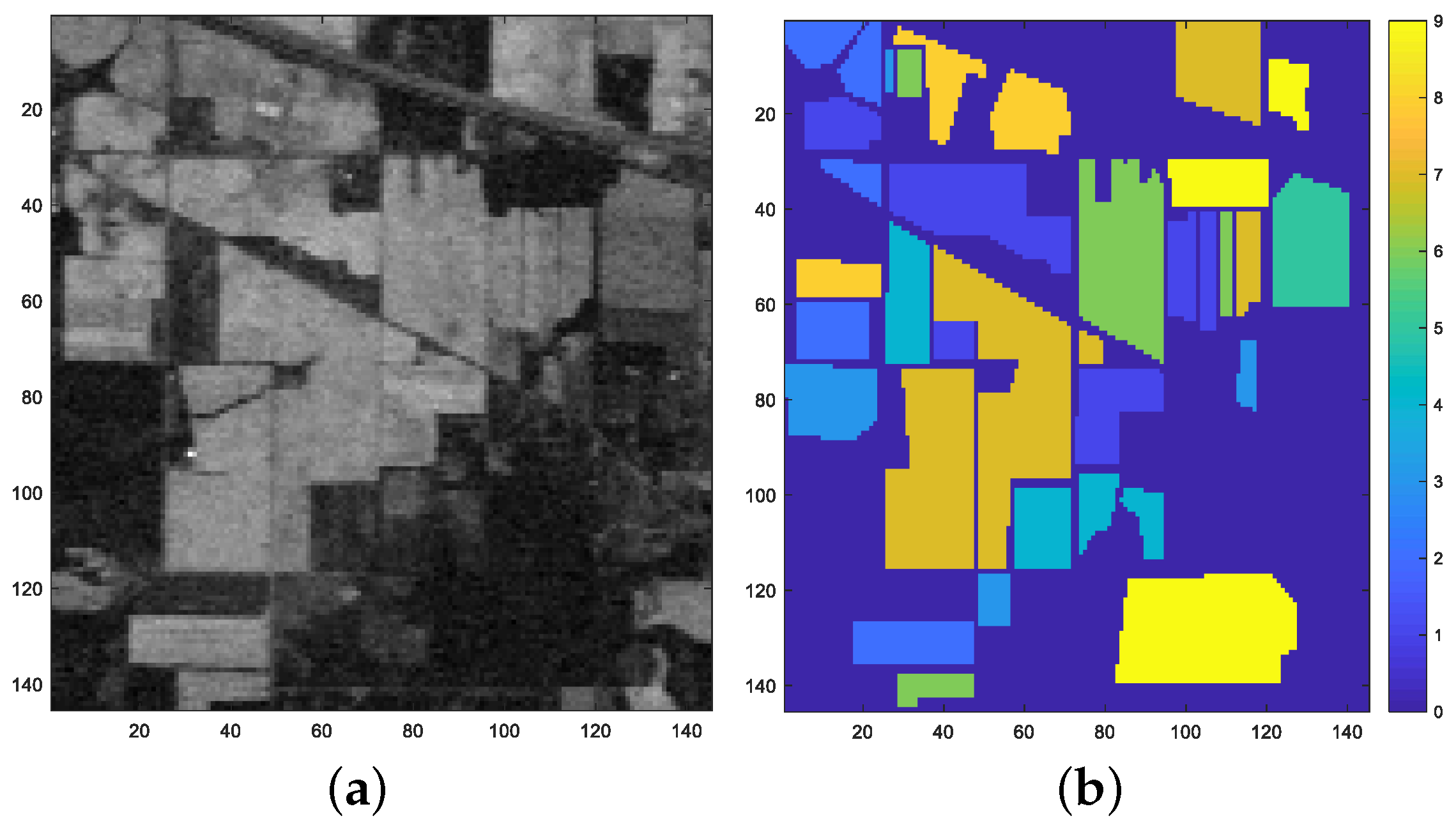
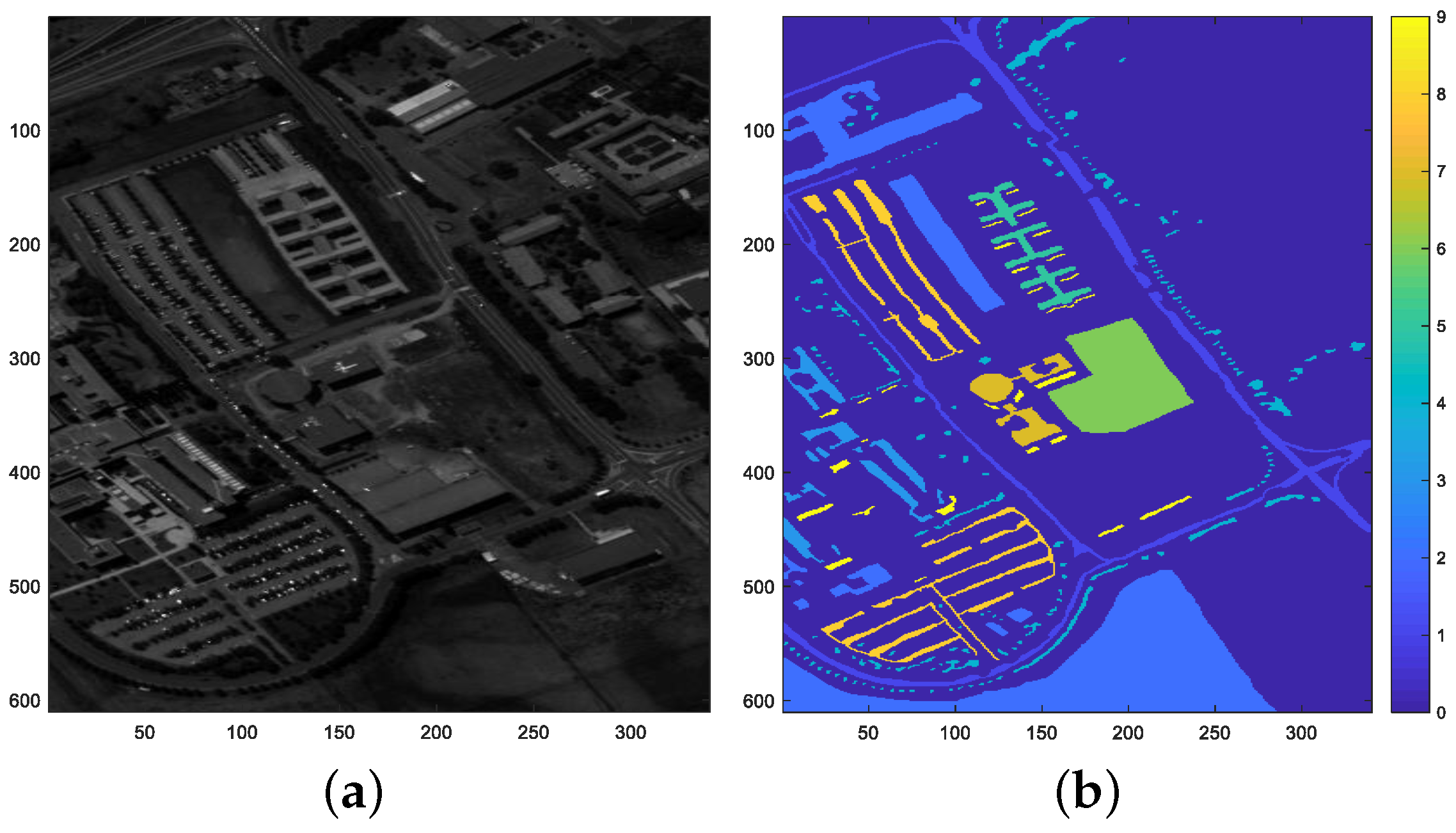
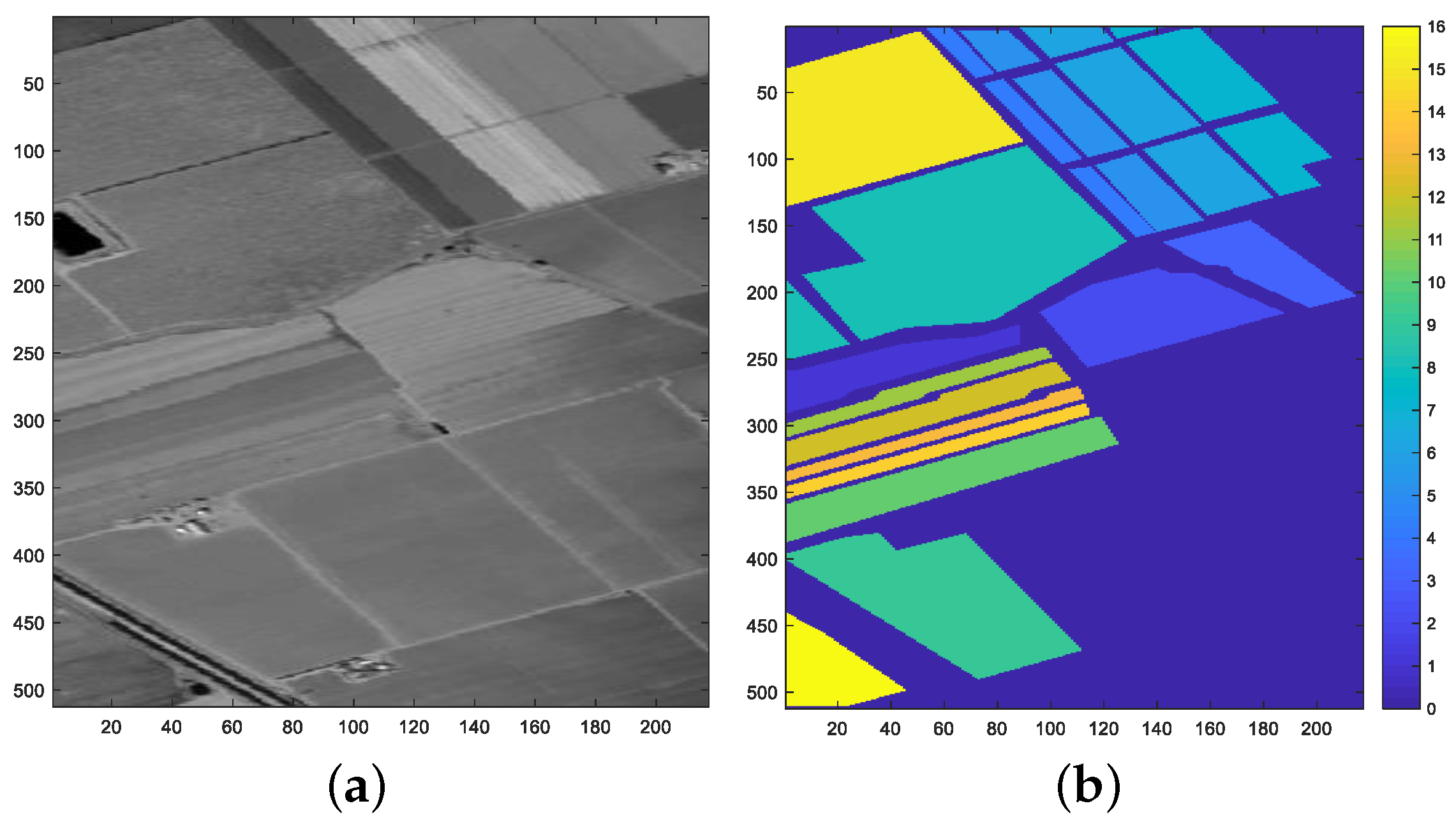
4.1. Indian Pine Dataset

The first hyperspectral image is the Indian Pines dataset, which has 145 × 145 pixels and 220 bands with a wavelength range from 400 to 2500 nm (Figure 3). In our experiments, bands 1-3, 103-112, 148-165, and 217-220 were removed due to atmospheric water vapor absorption and low signal to noise ratio (SNR) [14], leaving a total of 185 valid bands to be used. From the 16 land-cover classes available in the original ground truth, seven classes can be removed because of a lack of sufficient samples [14]. Thus, for the remaining nine classes (i.e., Corn-notill, Corn-mintill, Grass/Pasture, Grass/Trees, Haywindrowed, Soybeans-notill, Soybeans-meantill, Soybeans-clean and Woods), we randomly choose $10\%$ of the samples from each class to generate the training samples and the remainder are used as testing samples, then conduct classification experiments.

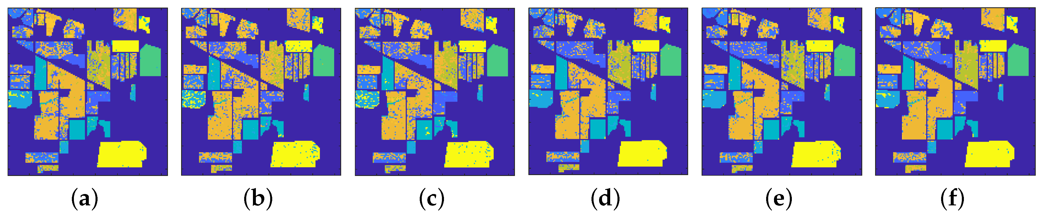
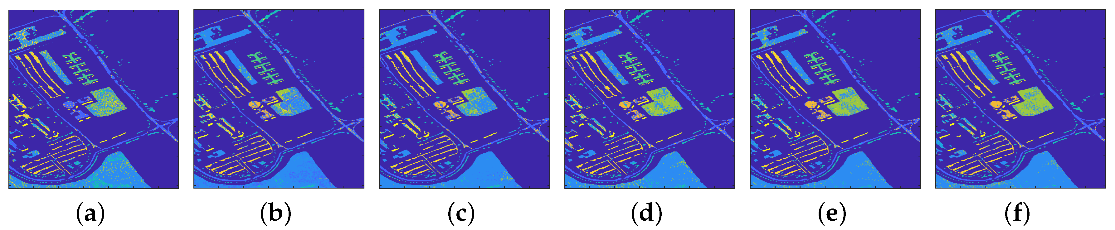
4.1.1. Classification Results

In the classification experiments, we first select some bands (i.e., features) by using different BS methods, then randomly split the samples into training and testing sets, and finally conduct pixel classification. To minimize the effect of stochastic process, we conduct experiments for five times, and the average results of the five runs are shown in Figure 4. Figure 4 shows the overall classification accuracies of using different numbers of selected bands, and the selected band number ranges from 2 to 50. Additionally, in Figure 5 and Figure 6, we provide the classification maps of using the fifteen bands selected by different BS methods. It can be seen from these results that the MRMR method shows the best overall classification performance among all the BS methods we used.

Specifically, we can see from Figure 4 that, all the classification accuracies of all the BS methods increase as the increase of the number of selected bands. When using the SVM classifier (Figure 4a), the MRMR method obtains the best overall performance, followed by ECA, OPBS, LCMVBCM and others. MRMR always outperforms the other competitors, and it obtains a significant increment on the classification accuracy when compared with other methods. For instance, in most cases, when compared with the second best method, i.e., ECA, the accuracy of MRMR is about 4% higher than that of the ECA method. As for the KNN classifier (Figure 4b), likewise, the MRMR method obtains the best overall classification results, followed by ECA, OPBS and others. When compared with ECA, the classification accuracy of the proposed method is still about 3% higher than that of ECA.

Figure 5 and Figure 6 show the classification maps of using the fifteen bands selected by different methods. The results show that the classification results of MRMR are much better than other five methods and further support the observations from Figure 4. Furthermore,

Table 1. Overall Accuracies and Average Accuracies of Using the Fifteen Bands Selected from the Indian Pine Dataset. (The bold denotes the best result).

	SVM		KNN
	OA (100%)	AA (100%)	OA (100%)	AA (100%)
1.MVPCA	67.74	67.99	59.95	61.19
2.LCMVBCC	64.39	63.82	54.25	54.90
3.LCMVBCM	70.48	72.02	62.60	63.52
4.ECA	77.45	76.99	70.62	69.41
5.OPBS	75.90	76.15	68.70	67.86
6.MRMR	81.32	82.70	72.94	72.86

lists the overall accuracy (OA) and average accuracy (AA) of classification. Overall accuracy is the ratio of correctly classified samples versus total samples, and average accuracy is the average of each accuracy per class. We can see from Table 1 that both the OAs and AAs of MRMR are much higher than those of other methods, which further verifies that the proposed method is superior to other methods.

Therefore, the experimental results on the Indian Pine dataset demonstrate that, the proposed method is an effective BS method and its selected bands can obtain much better classification performance than other competitors. Thence, this experiment has verified that the proposed method can select the band subset that well represent the whole image dataset and the selected bands are informative for classification.

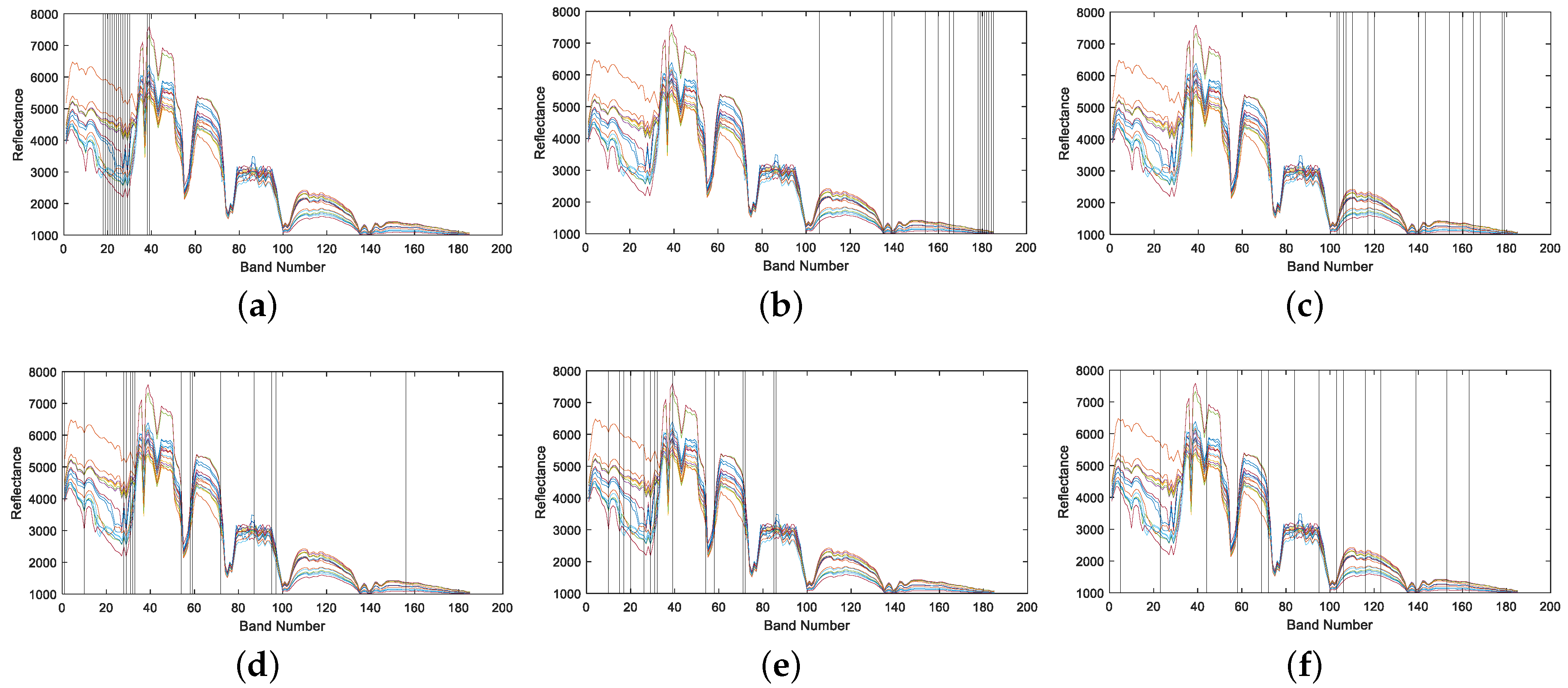
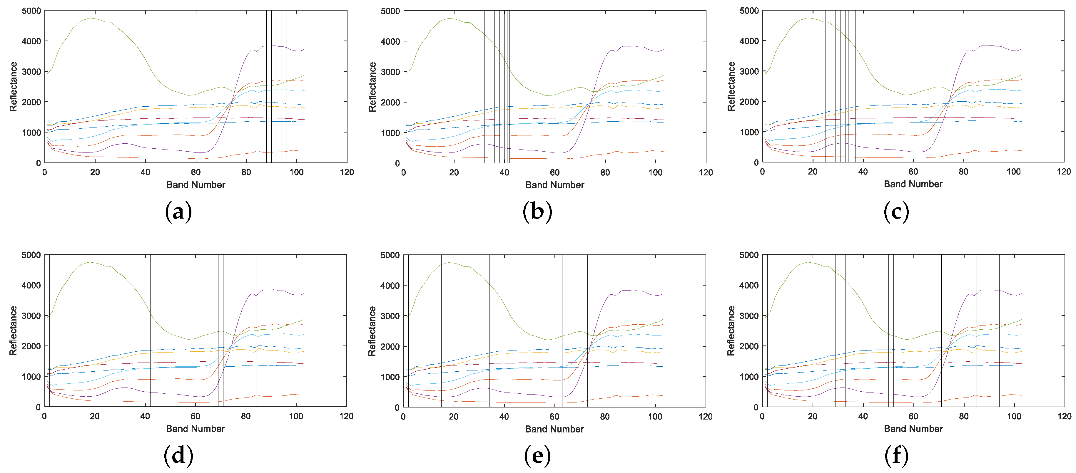
4.1.2. Band Correlation Comparison

BS methods should also take the band correlation among selected bands into consideration, because the high correlation among selected bands usually leads to much information redundancy and then deteriorates the pixel classification performances. In this section, we compare the average band correlation among the selected bands obtained by each BS methods. The overall band correlation of one band subset is measured by the average of correlation coefficients (ACC) of all the band pairs in this band set. Obviously, the larger the ACC is, the higher the band correlation is.

The ACCs of the fifteen selected bands of different BS methods are listed in

Table 2. Average band correlation and computing time for selecting fifteen bands from the Indian Pine dataset.

	Band Correlation (ACC)	Computing Time (s)
1.MVPCA	0.5950	0.2825
2.LCMVBCC	0.9816	3.0452
3.LCMVBCM	0.9882	2.5048
4.ECA	0.2988	1.6770
5.OPBS	0.1815	0.6376
6.MRMR	0.2179	1.7101

, from which we can see that the bands obtained by the MVPCA and LCMV-based methods are highly correlated, while the ones obtained by the other BS methods are with much lower correlation. Among all the BS methods, the OPBS method selects the bands with the lowest correlation, this occurs because that the OPBS method selects the band that is the most dissimilar (i.e., the lowest correlated) to the currently selected bands in each round. The bands selected by MRMR are also with low correlation, which is quite close to the correlation of the bands selected by OPBS. This demonstrates that the selection criterion of MRMR have well taken into account the band correlation among bands.

Furthermore, Figure 7 shows the 2D maps of the distribution of the bands along with the marked selected bands. In Figure 7, each curve denotes a spectrum of one category across a range of wavelengths, and the straight lines denotes the selected bands. For each category, the average of samples is used to represent this category. The 2D maps demonstrates that most of the bands selected by the MVPCA and LCMV-based methods are neighboring bands, while the ECA, OPBS and MRMR methods select much fewer neighboring bands. The neighboring hyperspectral bands are generally highly correlated with each other, so if a BS method selects many neighboring bands, the correlation among these selected bands would be significant. This is exactly the reason that the bands selected by the MVPCA and LCMV-based methods are with so high correlation. In practice, the high correlation among selected bands leads to much redundancy, which deteriorates the classification performances. For instance, we can observe from Table 1 and Table 2 that, the bands with high correlation usually corresponds to the low classification accuracies, and reducing the correlation among selected bands is helpful for improving the classification accuracies. Additionally, although ECA and OPBS select the bands that have quite low correlation, their classification performances are not as good as that of the proposed MRMR method, this occurs because that the selected bands obtained by these two methods are less informative than the bands obtained by the MRMR method, which indicates that the selection criterion of MRMR is more effective for finding the bands that have good representativeness.

To sum up, a good band selection method should pay sufficient attention on the band correlation among selected bands, and the band correlation comparison has verified that the proposed method can take into account the band correlation and select the bands with low redundancy.

4.1.3. Computing Time Comparison

The computing time of selecting 15 bands by different methods is also listed in Table 2, from which we can see that the MVPCA method runs the fastest, followed by OPBS, ECA, MRMR and other methods. Although the MVPCA method has better computational efficiency than the proposed method, considering that the MRMR method can achieve much better classification accuracy, it is acceptable that the MRMR method costs a little more time. When compared with the methods except for MVPCA, the MRMR method costs the medium time, so it also has a satisfactory computational efficiency and it enable to find the desired bands in a reasonable time. It should be pointed that, because the Indian Pine dataset is an image with a small number of pixels ($N=145\times 145=$ 21,025), the acceleration effect of the tricks introduced in Section 3.4 is not very significant. In fact, for the following dataset of larger size, the superiority of the proposed method on the computational efficiency would become more significant.

4.2. Pavia University Image

The second image is the Pavia University dataset, which is acquired by the ROSIS-3 optical sensor (Germany). The dataset has 103 spectral bands and there are $610\times 340$ pixels. There are nine classes in this image and all the classes are used in our experiments (Figure 8). For this dataset, we also randomly choose $10\%$ pixels for training and the rest for testing.

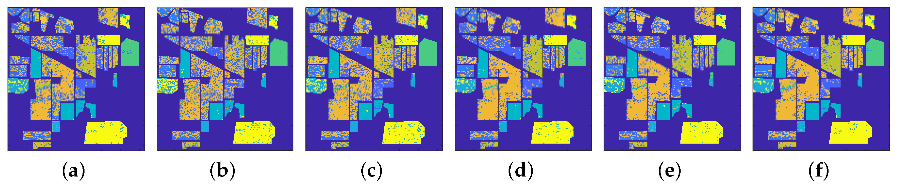
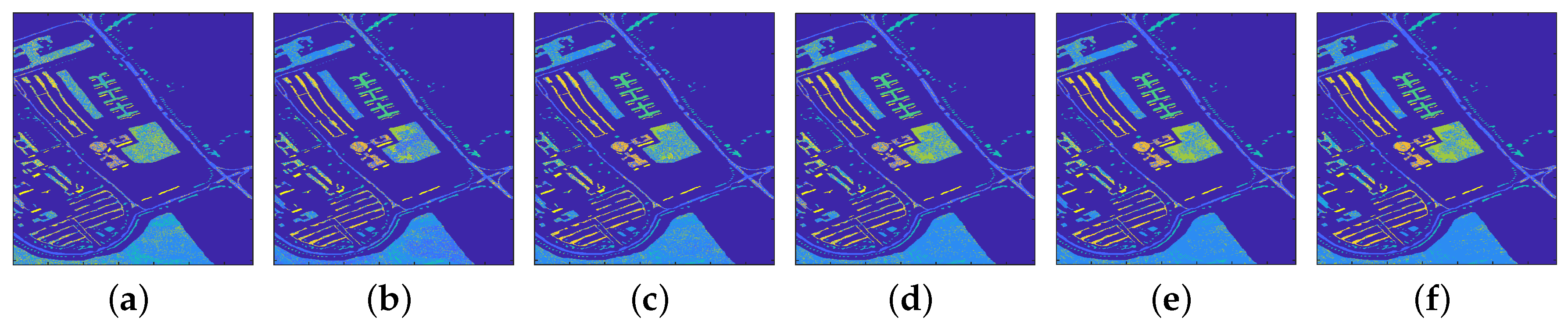
4.2.1. Classification Results

Likewise, different numbers of bands are selected from this dataset and the number ranges from 2 to 50. The average classification results of five runs are shown in Figure 9. Figure 10 and Figure 11 also show the classification maps of using the ten bands selected by different methods. It is evident that, for this dataset, the proposed method is also superior to other competitors.

It can be observed from Figure 9 that, the MRMR method performs the best, followed by the OPBS, ECA, MVPCA and LCMV-based methods. For the SVM classifier (Figure 9a), the MRMR method achieves the highest overall accuracies. In the case of selecting a small number of bands, e.g., less than 12 bands, the accuracy of the MRMR method is about 3% higher than the accuracy of the second best method (i.e., OPBS). When more bands are selected, the accuracy of the OPBS method increases significantly and is sometimes slightly higher than that of MRMR. As for the KNN classifier, likewise, MRMR achieves the highest classification accuracy, and OPBS also performs well. These two methods show a significant superiority relative to the remaining four methods. We also notice that when a large number of bands are selected, e.g., larger than 25 bands, most BS methods can obtain good classification performances. Since the major purpose of BS is selecting a few informative bands to improve the computational efficiency and ease the storage burden, fewer bands with a good classification performance is encouraged. The proposed method achieves the best classification performance and shows a significant superiority to other competitive methods when selecting quite few bands (e.g., less than 15 bands), which indicates that the proposed method is valuable.

Furthermore, we can observe from Figure 10 and Figure 11 that the classification maps of MRMR are the most correct.

Table 3. Overall Classification Accuracies and Average Classification Accuracies of Using the Ten Bands Selected from the Pavia University Dataset. (The bold denotes the best result).

	SVM		KNN
	OA (100%)	AA (100%)	OA (100%)	AA (100%)
1.MVPCA	70.96	62.83	63.87	59.09
2.LCMVBCC	69.08	64.36	60.69	62.52
3.LCMVBCM	77.19	70.20	68.27	68.27
4.ECA	83.89	79.96	76.62	72.65
5.OPBS	86.58	83.62	80.87	78.38
6.MRMR	90.15	87.78	83.76	82.57

further lists the OAs and AAs of using the ten bands obtained by different methods. Similar to the results on the Indian Pine dataset, MRMR again acquires the highest OAs and AAs. These results further support the observations from Figure 9 and we can conclude that the MRMR method is superior to others.

4.2.2. Band Correlation Comparison

Table 4. Average band correlation and computing time for selecting fifteen bands from the Pavia University dataset.

	Band Correlation (ACC)	Computing Time (s)
1.MVPCA	0.9981	1.1549
2.LCMVBCC	0.9880	5.7662
3.LCMVBCM	0.9934	4.3998
4.ECA	0.6223	15.2934
5.OPBS	0.5267	2.5998
6.MRMR	0.5788	2.3671

lists the average band correlation of the ten selected bands. Similarly, for this dataset, the bands selected by the MVPCA, LCMV-based methods are still highly correlated, whereas the other BS methods select the bands with lower correlation. Figure 12 shows that the MVPCA, LCMV-based methods select many neighboring bands, while the other three methods select less neighboring bands. It is worth noting that, although the bands selected by ECA and OPBS are not with high correlation, the distributions of these two methods’ selected bands are more centralized than that of the MRMR method. In other words, the distribution of the bands selected by MRMR is more dispersed. For instance, most bands selected by ECA are distributed among the bands 1–10 and 65–85; and about one half of the selected bands of OPBS belong to the bands 1–10; while the bands selected by MRMR are much more isolated. By observing the spectrums of categories, we can find that, for ECA and OPBS, some selected bands like bands 74 and 73 may be little useful for discriminating most categories in the dataset, and some bands like bands 1–4 are actually similar to each other, which means some selected bands of OPBS and ECA may be lowly representative (e.g., bands 73 and 74) or redundant (e.g., bands 1–4). On the contrary, the distribution of the selected bands of MRMR is more dispersed, and each selected band is useful for discriminating categories, so we can intuitively conclude that the selected bands of MRMR is more useful for classification. Some similar results can be also observed in Figure 7. Therefore, it can be concluded according to the classification results and band correlation comparison that the selected bands obtained by the MRMR method are not only highly representative but also lowly redundant.

4.2.3. Computing Time Comparison

Table 4 also gives the computing time of selecting ten bands by different methods. For this dataset, MVPCA costs the shortest time, followed by MRMR, OPBS, and other methods. We can see that the computing time of MRMR is only higher than that of MVPCA and is close to that of OPBS, this occurs because that the Pavia University dataset is with a huge number of pixels ($N=610\times 340=$ 207,400), so the accelerating effect of the tricks introduced in Section 3.4 becomes more significant. When compared with the results on the Indian Pine dataset, it can be concluded that the proposed method has a more significant superiority in computational efficiency when dealing with large-scale images. Therefore, the experimental results on this dataset further proves that the MRMR method has a satisfactory computational efficiency, especially when processing the large-scale images.

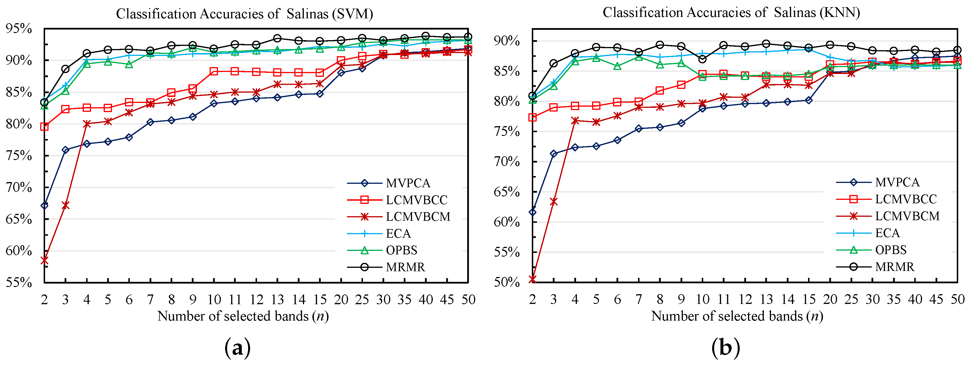
4.3. Salinas Dataset

The third image was also collected by the 224-band AVIRIS sensor over Salinas Valley, California, and was characterized by a high spatial resolution (3.7-meter pixels) (Figure 13) [45]. The dataset has a medium size of $512\times 217$ pixels, and the spectral range is from 370 to 2507 nm. In our experiments, all the 16 classes in the Salinas dataset are used.

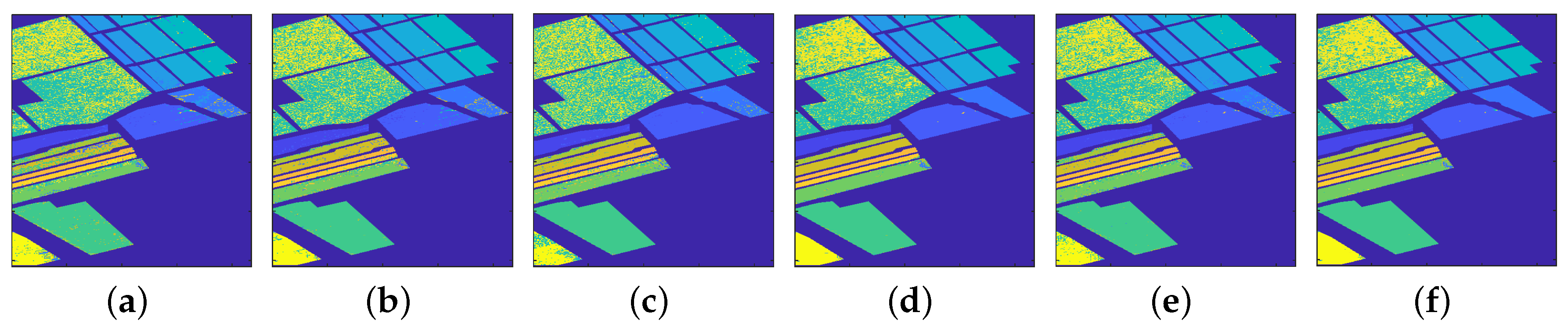
4.3.1. Classification Results

The classification results on this dataset are shown in Figure 14, Figure 15 and Figure 16 and

Table 5. Overall Classification Accuracies and Average Classification Accuracies of Using the Fifteen Bands Selected from the Salinas Dataset. (The bold denotes the best result).

	SVM		KNN
	OA (100%)	AA (100%)	OA (100%)	AA (100%)
1.MVPCA	84.75	87.78	80.16	83.56
2.LCMVBCC	88.06	90.91	84.08	86.57
3.LCMVBCM	86.36	87.02	82.65	85.44
4.ECA	92.16	95.67	88.58	92.87
5.OPBS	91.72	95.34	84.54	88.77
6.MRMR	93.02	96.31	88.83	93.13

. It is evident that, for this dataset, the proposed method is also superior to other competitors.

The classification accuracy curves in Figure 14 shows all methods perform well for this dataset, especially the MRMR, OPBS and ECA methods. Although OPBS and ECA performs quite well, we can see that the proposed method still obtains the best results in most cases. We also notice that, for this dataset, the proposed can obtain quite good classification performances when selecting quite a limited number of bands (e.g., less than 5 bands). Furthermore, the results in Table 5 demonstrate that the proposed method obtains the highest OAs and AAs for both the two classifiers, and correspondingly, the associated classification maps of the proposed method is the most similar to the ground truth maps among all the classification maps (Figure 15 and Figure 16). Therefore, these classification results on Salinas dataset further indicate that the proposed method is effective for finding the bands that are informative for classification.

4.3.2. Band Correlation Comparison

Likewise,

Table 6. Average band correlation and computing time for selecting fifteen bands from the Salinas dataset.

	Band Correlation (ACC)	Computing Time (s)
1.MVPCA	0.9976	1.1549
2.LCMVBCC	0.6282	5.7662
3.LCMVBCM	0.7001	4.3998
4.ECA	0.4509	15.2934
5.OPBS	0.3728	2.5998
6.MRMR	0.3039	2.3671

lists the average band correlation of the fifteen selected bands. For this dataset, the bands selected by the MVPCA, LCMV-based methods are still highly correlated, whereas the other BS methods select the bands with lower correlation. For this dataset, the proposed method’s selected bands have the lowest average correlation, and we can also see from Figure 17 that the MVPCA, LCMV-based methods select many neighboring bands, while the selected bands of other methods are more dispersed. It is worth noting that when compared with the OPBS and ECA methods, the distribution of the bands selected by the proposed method is also more dispersed and it can be intuitively seen that the bands selected by the proposed method are more reasonable.

4.3.3. Computing Time Comparison

The computing time of selecting ten bands by different methods is also listed in Table 6. The Salinas dataset has more pixels than the previous Indian Pine dataset, so the proposed method should show good performance in terms of the computational efficiency. We can see that MVPCA costs the shortest time, followed by MRMR, OPBS, and other methods. The computing time of MRMR is only higher than that of MVPCA and is slighted shorter than that of OPBS, which further indicates that the accelerating effect of the tricks introduced in Section 3.4 is effective. Therefore, the experimental results on this dataset also proves that the MRMR method has a satisfactory computational efficiency, especially when processing the large-scale images.

4.4. Summary

In the end, some important results can be summarized from all the experiments. In unsupervised band selection, the BS methods should evaluate the representativeness and the correlation among selected bands jointly. The proposed method explicitly designs two metrics for evaluating these two factors and then combine them into an effective selection criterion. Experimental results have verified that the selected bands obtained by the MRMR method are not only informative for pixel classification but also with low correlation. Among all the methods we used, the MRMR method shows the best performance of classification, it even outperforms the state-of-art methods like OPBS and ECA. When compared with the similar methods, namely, the OPBS and LCMV-based methods, the MRMR method is much superior to them, which demonstrates the effectiveness of the proposed selection criterion. Furthermore, considering that BS is to select several bands to replace the whole dataset, it is preferable that the BS methods select fewer bands but maintain a satisfactory classification performance. When selecting quite few bands, the MRMR method still obtains quite good classification performances, so this method is valuable. Finally, thanks to the accelerating tricks for computing the orthogonal projection, the MRMR method has a satisfactory computational efficiency. In conclusion, the effectiveness of the proposed method has been verified.

5. Conclusions

In this paper, we proposed an unsupervised feature selection approach based on maximizing representativeness and minimizing redundancy to select some important bands from hyperspectral images. The MRMR method aims to find the band subset that has the maximum representativeness and the minimum redundancy. The representativeness of one band subset is measured by the distances of the remaining bands to their orthogonal projections onto the hyperplane which is spanned by the bands of the subset. The redundancy of one band subset is measured by the average correlation coefficient of the bands in this subset. To find the subset with good representativeness and low redundancy, an effective evolutionary algorithm named the Immune Clone Selection (ICS) is applied as the searching strategy. Moreover, to ensure that the proposed method can be used in practical applications, two useful tricks are introduced to accelerate the computation of the subsets’ representativeness, any of them can be applied to reduce the computational burden of the MRMR method. The experimental results on three different datasets have verified that the proposed method is a highly effective BS method with a satisfactory computational efficiency. Finally, our future research interest is to find the other effective metrics to evaluate the representativeness and redundancy for improving the performance of the proposed method.

References

1. Jolliffe, I.T. Principal Component Analysis. In Principal Component Analysis; Springer: Berlin/Heidelberg, Germany, 1986; pp. 115–128. [Google Scholar]
2. Khan, Z.; Shafait, F.; Mian, A. Joint Group Sparse PCA for Compressed Hyperspectral Imaging. IEEE Trans. Image Process. 2015, 24, 4934–4942. [Google Scholar] [CrossRef] [PubMed]
3. Lee, D.D.; Seung, H.S. Learning the parts of objects by non-negative matrix factorization. Nature 1999, 401, 788–791. [Google Scholar] [CrossRef] [PubMed]
4. Hyvärinen, A.; Hurri, J.; Hoyer, P.O. Independent component analysis. Natural Image Statistics; Springer Science & Business Media: New York, NY, USA, 2009; pp. 151–175. [Google Scholar]
5. Roweis, S.T.; Saul, L.K. Nonlinear dimensionality reduction by locally linear embedding. Science 2000, 290, 2323–2326. [Google Scholar] [CrossRef] [PubMed]
6. Prabukumar, M.; Shrutika, S. Band clustering using expectation–maximization algorithm and weighted average fusion-based feature extraction for hyperspectral image classification. J. Appl. Remote Sens. 2018, 12, 046015. [Google Scholar] [CrossRef]
7. Prabukumar, M.; Sawant, S.; Samiappan, S.; Agilandeeswari, L. Three-dimensional discrete cosine transform-based feature extraction for hyperspectral image classification. J. Appl. Remote Sens. 2018, 12, 046010. [Google Scholar] [CrossRef]
8. Taşkın, G.; Kaya, H.; Bruzzone, L. Feature Selection Based on High Dimensional Model Representation for Hyperspectral Images. IEEE Trans. Image Process. 2017, 26, 2918–2928. [Google Scholar] [CrossRef] [PubMed]
9. Persello, C.; Bruzzone, L. Kernel-Based Domain-Invariant Feature Selection in Hyperspectral Images for Transfer Learning. IEEE Trans. Geosci. Remote Sens. 2016, 54, 2615–2626. [Google Scholar] [CrossRef]
10. Chang, C.I.; Wang, S. Constrained band selection for hyperspectral imagery. IEEE Trans. Geosci. Remote Sens. 2006, 44, 1575–1585. [Google Scholar] [CrossRef]
11. Yuan, Y.; Zheng, X.; Lu, X. Discovering diverse subset for unsupervised hyperspectral band selection. IEEE Trans. Image Process. 2017, 26, 51–64. [Google Scholar] [CrossRef] [PubMed]
12. Guo, B.; Gunn, S.R.; Damper, R.I.; Nelson, J.D. Band selection for hyperspectral image classification using mutual information. IEEE Geosci. Remote Sens. Lett. 2006, 3, 522–526. [Google Scholar] [CrossRef]
13. Chang, C.I.; Du, Q.; Sun, T.L.; Althouse, M.L. A joint band prioritization and band-decorrelation approach to band selection for hyperspectral image classification. IEEE Trans. Geosci. Remote Sens. 1999, 37, 2631–2641. [Google Scholar] [CrossRef] [Green Version]
14. Liu, X.S.; Ge, L.; Wang, B.; Zhang, L.M. An unsupervised band selection algorithm for hyperspectral imagery based on maximal information. J. Infrared Millim. Waves 2012, 31, 166–176. [Google Scholar] [CrossRef]
15. Sheffield, C. Selecting band combinations from multispectral data. Photogramm. Eng. Remote Sens. 1985, 51, 681–687. [Google Scholar]
16. Zhang, W.; Li, X.; Zhao, L. Hyperspectral band selection based on triangular factorization. J. Appl. Remote Sens. 2017, 11, 025007. [Google Scholar] [CrossRef]
17. Zare, A.; Gader, P. Hyperspectral band selection and endmember detection using sparsity promoting priors. IEEE Geosci. Remote Sens. Lett. 2008, 5, 256–260. [Google Scholar] [CrossRef]
18. Zhang, W.; Li, X.; Dou, Y.; Zhao, L. Fast linear-prediction-based band selection method for hyperspectral image analysis. J. Appl. Remote Sens. 2018, 12, 016027. [Google Scholar] [CrossRef]
19. Zhang, W.; Li, X.; Dou, Y.; Zhao, L. A Geometry-Based Band Selection Approach for Hyperspectral Image Analysis. IEEE Trans. Geosci. Remote Sens. 2018, 56, 4318–4333. [Google Scholar] [CrossRef]
20. Geng, X.; Sun, K.; Ji, L.; Zhao, Y. A fast volume-gradient-based band selection method for hyperspectral image. IEEE Trans. Geosci. Remote Sens. 2014, 52, 7111–7119. [Google Scholar] [CrossRef]
21. Yu, C.; Lee, L.; Chang, C.; Xue, B.; Song, M.; Chen, J. Band-Specified Virtual Dimensionality for Band Selection: An Orthogonal Subspace Projection Approach. IEEE Trans. Geosci. Remote Sens. 2018, 56, 2822–2832. [Google Scholar] [CrossRef]
22. Wang, L.; Jia, X.; Zhang, Y. A novel geometry-based feature-selection technique for hyperspectral imagery. IEEE Geosci. Remote Sens. Lett. 2007, 4, 171–175. [Google Scholar] [CrossRef]
23. Sun, K.; Geng, X.; Ji, L. Exemplar component analysis: A fast band selection method for hyperspectral imagery. IEEE Geosci. Remote Sens. Lett. 2015, 12, 998–1002. [Google Scholar]
24. Ahmad, M.; Haq, D.I.U.; Mushtaq, Q.; Sohaib, M. A new statistical approach for band clustering and band selection using K-means clustering. IACSIT Int. J. Eng. Technol. 2011, 3, 606–614. [Google Scholar]
25. Jia, S.; Tang, G.; Zhu, J.; Li, Q. A Novel Ranking-Based Clustering Approach for Hyperspectral Band Selection. IEEE Trans. Geosci. Remote Sens. 2016, 54, 88–102. [Google Scholar] [CrossRef]
26. Li, H.; Xiang, S.; Zhong, Z.; Ding, K.; Pan, C. Multicluster Spatial-Spectral Unsupervised Feature Selection for Hyperspectral Image Classification. IEEE Geosci. Remote Sens. Lett. 2015, 12, 1660–1664. [Google Scholar] [CrossRef]
27. Qian, Y.; Yao, F.; Jia, S. Band selection for hyperspectral imagery using affinity propagation. IET Comput. Vis. 2009, 3, 213–222. [Google Scholar] [CrossRef]
28. Wang, Q.; Lin, J.; Yuan, Y. Salient band selection for hyperspectral image classification via manifold ranking. IEEE Trans. Neural Netw. Learn. Syst. 2016, 27, 1279–1289. [Google Scholar] [CrossRef]
29. Sun, K.; Geng, X.; Ji, L. A new sparsity-based band selection method for target detection of hyperspectral image. IEEE Geosci. Remote Sens. Lett. 2015, 12, 329–333. [Google Scholar]
30. Xenaki, S.D.; Koutroumbas, K.D.; Rontogiannis, A.A.; Sykioti, O.A. A new sparsity-aware feature selection method for hyperspectral image clustering. In Proceedings of the 2015 IEEE International Geoscience and Remote Sensing Symposium (IGARSS), Milan, Italy, 26–31 July 2015; pp. 445–448. [Google Scholar]
31. De Castro, L.N.; Von Zuben, F.J. Learning and optimization using the clonal selection principle. IEEE Trans. Evol. Comput. 2002, 6, 239–251. [Google Scholar] [CrossRef]
32. Chang, C.I. Hyperspectral Imaging: Techniques for Spectral Detection and Classification; Springer Science & Business Media: New York, NY, USA, 2003; Volume 1. [Google Scholar]
33. Pudil, P.; Ferri, F.J.; Novovicova, J.; Kittler, J. Floating search methods for feature selection with nonmonotonic criterion functions. In Proceedings of the 12th IAPR International Conference on Pattern Recognition, Jerusalem, Israel, 9–13 October 1994; Volume 2, pp. 279–283. [Google Scholar]
34. Zhang, X.D. Matrix Analysis and Applications; Cambridge University Press: Cambridge, UK, 2017. [Google Scholar]
35. Jain, A.; Zongker, D. Feature selection: Evaluation, application, and small sample performance. IEEE Trans. Pattern Anal. Mach. Intell. 1997, 19, 153–158. [Google Scholar] [CrossRef]
36. Somol, P.; Pudil, P.; Kittler, J. Fast branch & bound algorithms for optimal feature selection. IEEE Trans. Pattern Anal. Mach. Intell. 2004, 26, 900–912. [Google Scholar] [CrossRef]
37. Gen, M.; Cheng, R. Genetic Algorithms and Engineering Optimization; John Wiley & Sons: Hoboken, NJ, USA, 2000; Volume 7. [Google Scholar]
38. Serpico, S.B.; Bruzzone, L. A new search algorithm for feature selection in hyperspectral remote sensing images. IEEE Trans. Geosci. Remote Sens. 2001, 39, 1360–1367. [Google Scholar] [CrossRef]
39. Furcy, D.; Koenig, S. Limited discrepancy beam search. In Proceedings of the 19th International Joint Conference on Artificial Intelligence (IJCAI’05), Edinburgh, Scotland, UK, 30 July–5 August 2005; pp. 125–131. [Google Scholar]
40. Kennedy, J. Particle swarm optimization. In Encyclopedia of Machine Learning; Springer: Berlin/Heidelberg, Germany, 2011; pp. 760–766. [Google Scholar]
41. Chang, C.I.; Du, Q. Estimation of number of spectrally distinct signal sources in hyperspectral imagery. IEEE Trans. Geosci. Remote Sens. 2004, 42, 608–619. [Google Scholar] [CrossRef]
42. Melgani, F.; Bruzzone, L. Classification of hyperspectral remote sensing images with support vector machines. IEEE Trans. Geosci. Remote Sens. 2004, 42, 1778–1790. [Google Scholar] [CrossRef] [Green Version]
43. Devroye, L.; Györfi, L.; Lugosi, G. A Probabilistic Theory of Pattern Recognition; Springer Science & Business Media: New York, NY, USA, 2013; Volume 31. [Google Scholar]
44. Rifkin, R.; Klautau, A. In defense of one-vs-all classification. J. Mach. Learn. Res. 2004, 5, 101–141. [Google Scholar]
45. Dópido, I.; Li, J.; Gamba, P.; Plaza, A. A new hybrid strategy combining semisupervised classification and unmixing of hyperspectral data. IEEE J. Sel. Top. Appl. Earth Obs. Remote Sens. 2014, 7, 3619–3629. [Google Scholar] [CrossRef]
Figure 1. An intuitive explanation of orthogonal projection. (a) The vector x 0 cannot be linearly represented by the vectors x 1 and x 2 . (b) The vector x 0 can be linearly represented by the vectors x 1 and x 2 .
Remotesensing 11 01341 g001
Figure 2. A 3-D example for illustrating the rationality of Equation (7). The round marks denote the bands of the remaining subset Y , and the hyperplane is spanned by X .
Remotesensing 11 01341 g002
Figure 3. Band 170 and the ground truth of the Indian Pine dataset. (a) Band 170. (b) The ground truth map (label 0 denotes background).
Remotesensing 11 01341 g003
Figure 4. Overall classification accuracies of using the bands selected by different BS methods from the Indian Pine dataset. (a) SVM (b) KNN.
Remotesensing 11 01341 g004
Figure 5. SVM classification maps of using the fifteen bands selected by different methods from the Indian Pine dataset. (a) MVPCA (b) LCMVBCC (c) LCMVBCM (d) ECA (e) OPBS (f) MRMR.
Remotesensing 11 01341 g005
Figure 6. KNN classification maps of using the fifteen bands selected by different methods from the Indian Pine dataset. (a) MVPCA (b) LCMVBCC (c) LCMVBCM (d) ECA (e) OPBS (f) MRMR.
Remotesensing 11 01341 g006
Figure 7. Spectrums of the categories on the Indian Pine dataset. The straight lines denote the bands selected by different BS methods. (a) MVPCA (b) LCMVBCC (c) LCMVBCM (d) ECA (e) OPBS (f) MRMR.
Remotesensing 11 01341 g007
Figure 8. Band 50 and the ground truth of the Pavia University dataset. (a) Band 50. (b) The ground truth (label 0 denotes background).
Remotesensing 11 01341 g008
Figure 9. Overall classification accuracies of using the bands selected by different BS methods from the Pavia University dataset. (a) SVM (b) KNN.
Remotesensing 11 01341 g009
Figure 10. SVM classification maps of using the ten bands selected by different methods from the Pavia University dataset. (a) MVPCA (b) LCMVBCC (c) LCMVBCM (d) ECA (e) OPBS (f) MRMR.
Remotesensing 11 01341 g010
Figure 11. KNN classification maps of using the ten bands selected by different methods from the Pavia University dataset. (a) MVPCA (b) LCMVBCC (c) LCMVBCM (d) ECA (e) OPBS (f) MRMR.
Remotesensing 11 01341 g011
Figure 12. Spectrums of the categories on the Pavia University dataset. The straight lines denote the bands selected by different BS methods. (a) MVPCA (b) LCMVBCC (c) LCMVBCM (d) ECA (e) OPBS (f) MRMR.
Remotesensing 11 01341 g012
Figure 13. Band 100 and the ground truth of the Salinas dataset. (a) Band 100. (b) The ground truth (label 0 denotes background).
Remotesensing 11 01341 g013
Figure 14. Overall classification accuracies of using the bands selected by different BS methods from the Salinas dataset. (a) SVM (b) KNN.
Remotesensing 11 01341 g014
Figure 15. SVM classification maps of using the ten bands selected by different methods from the Salinas dataset. (a) MVPCA (b) LCMVBCC (c) LCMVBCM (d) ECA (e) OPBS (f) MRMR.
Remotesensing 11 01341 g015
Figure 16. KNN classification maps of using the ten bands selected by different methods from the Salinas dataset. (a) MVPCA (b) LCMVBCC (c) LCMVBCM (d) ECA (e) OPBS (f) MRMR.
Remotesensing 11 01341 g016
Figure 17. Spectrums of the categories on the Salinas dataset. The straight lines denote the bands selected by different BS methods. (a) MVPCA (b) LCMVBCC (c) LCMVBCM (d) ECA (e) OPBS (f) MRMR.
Remotesensing 11 01341 g017