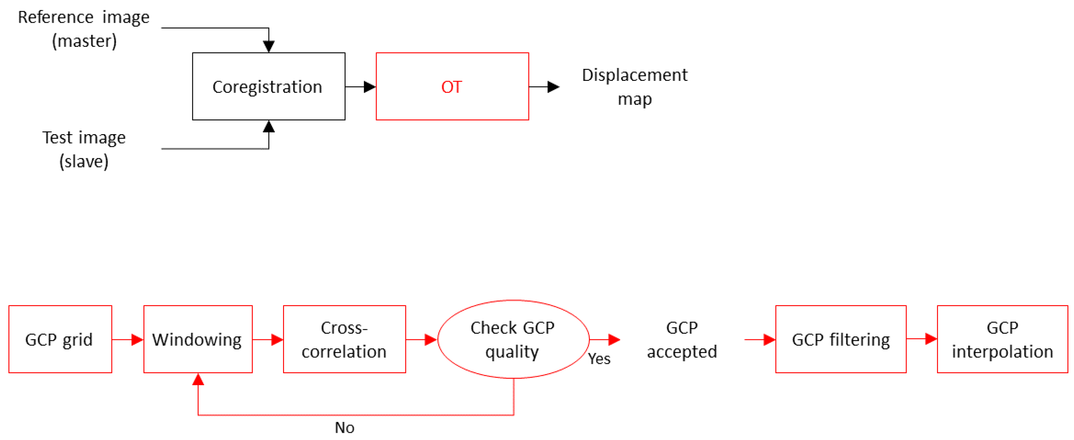
Figure 1.
Block diagram of the implemented frequency-domain offset tracking (OT) technique. The lower diagram is an exploded view of the OT processing block.
Figure 1.
Block diagram of the implemented frequency-domain offset tracking (OT) technique. The lower diagram is an exploded view of the OT processing block.
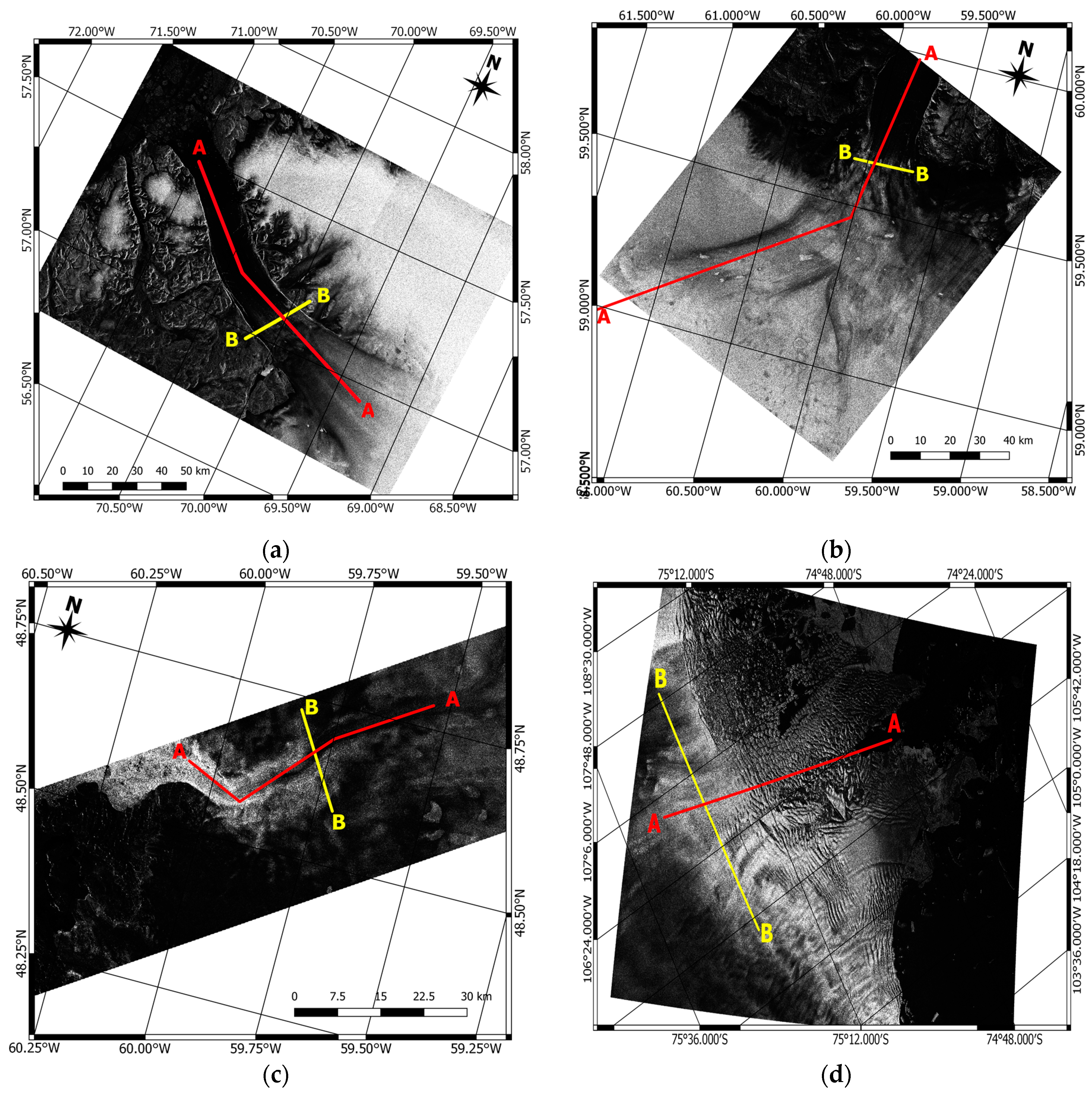
Figure 2.
SAR images (all acquired in right ascending orbit) of the test sites with the corresponding analyzed transects (AA—along flow, BB—across flow). (a) Petermann glacier, (b) Nioghalvfjerdsfjorden, (c) Jakobshavn Isbræ and (d) Thwaites glacier.
Figure 2.
SAR images (all acquired in right ascending orbit) of the test sites with the corresponding analyzed transects (AA—along flow, BB—across flow). (a) Petermann glacier, (b) Nioghalvfjerdsfjorden, (c) Jakobshavn Isbræ and (d) Thwaites glacier.
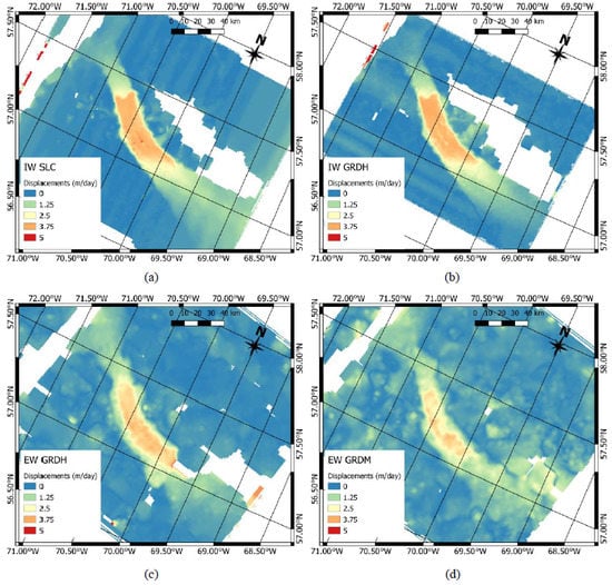
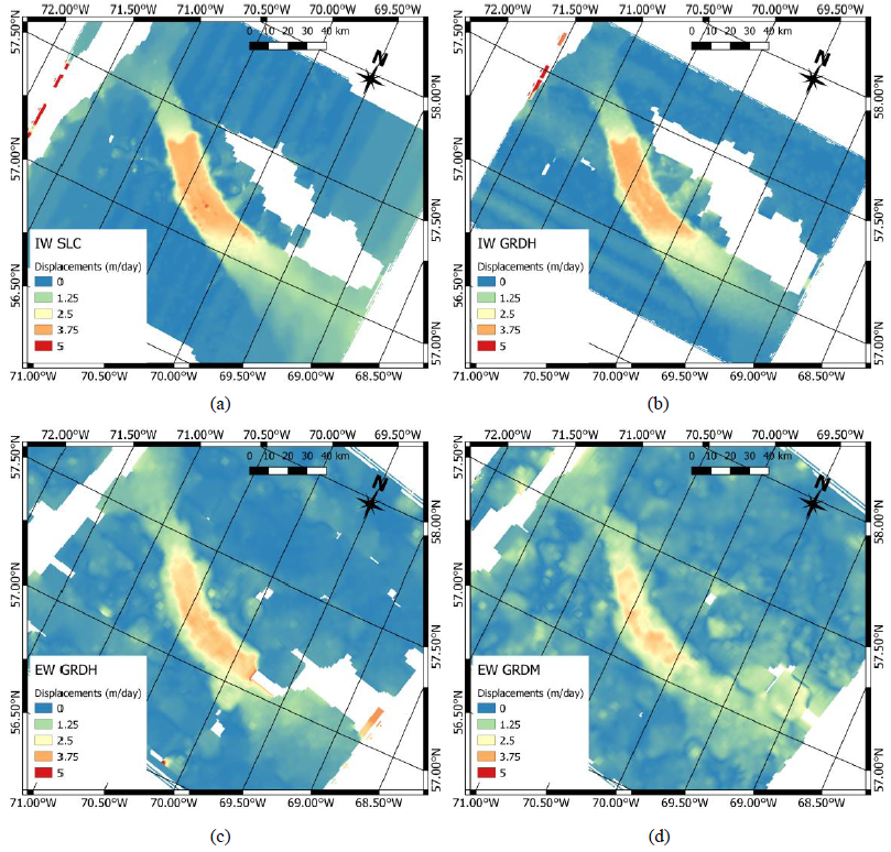
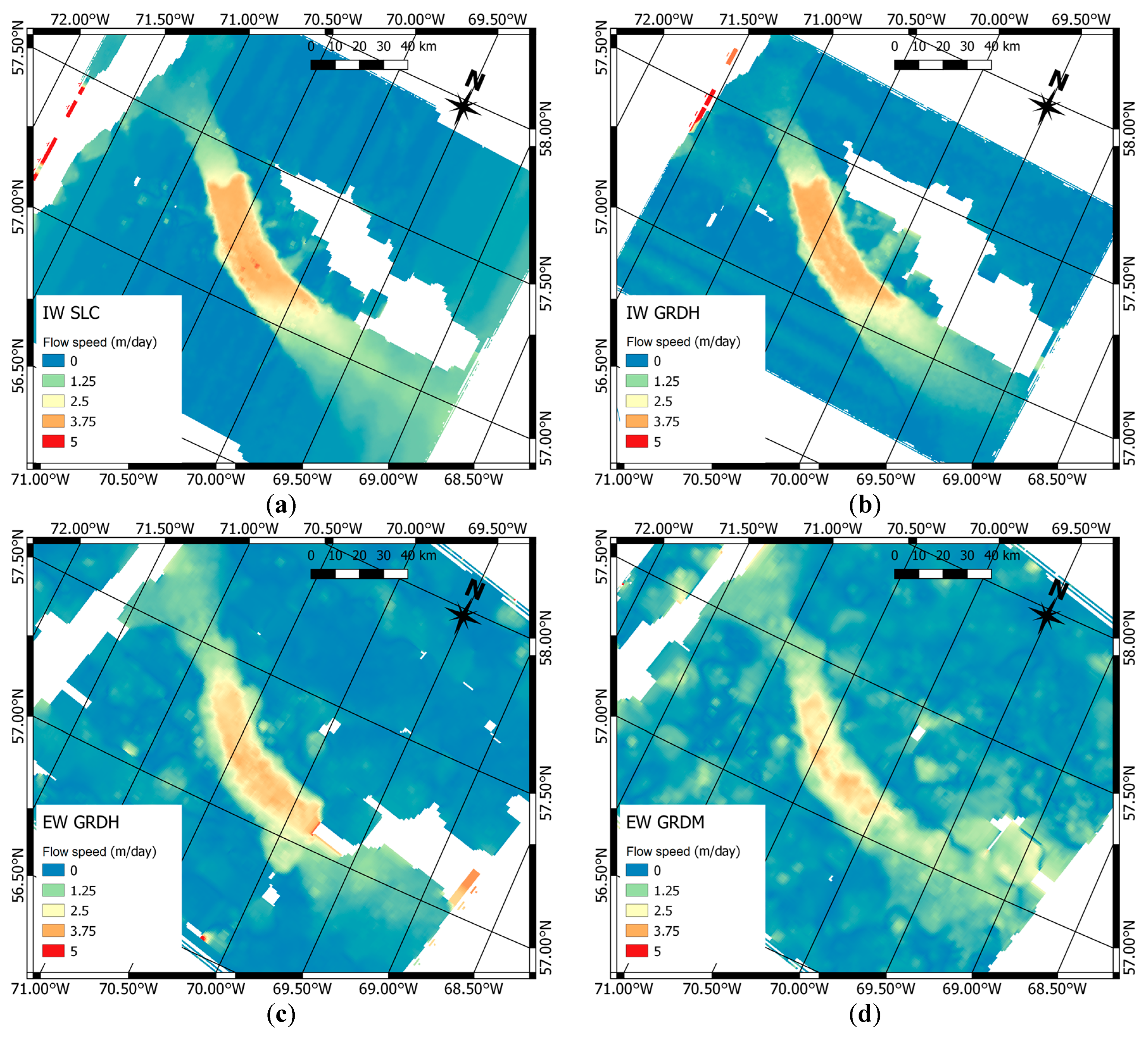
Figure 3.
PG, flow speed maps obtained using (a) IW SLC, (b) IW GRDH, (c) EW GRDH and (d) EW GRDM images. Observation periods are 6–12 January 2017 for IW images and 1–13 April for EW images.
Figure 3.
PG, flow speed maps obtained using (a) IW SLC, (b) IW GRDH, (c) EW GRDH and (d) EW GRDM images. Observation periods are 6–12 January 2017 for IW images and 1–13 April for EW images.
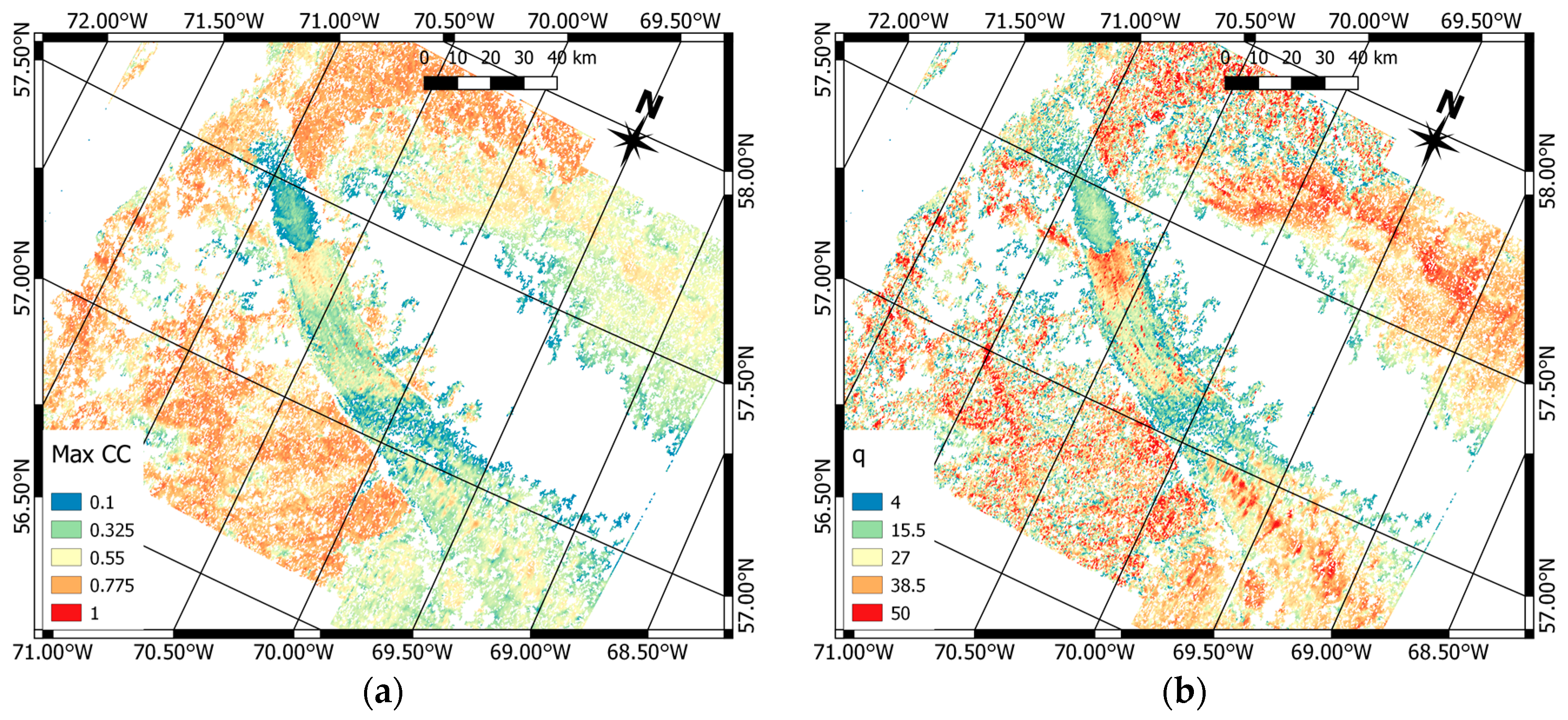
Figure 4.
PG, quality parameters maps obtained by processing the IW SLC pair 6–12 January 2017. (a) Maximum correlation. (b) Ratio between the peak and the background of the correlation matrix (q-parameter).
Figure 4.
PG, quality parameters maps obtained by processing the IW SLC pair 6–12 January 2017. (a) Maximum correlation. (b) Ratio between the peak and the background of the correlation matrix (q-parameter).
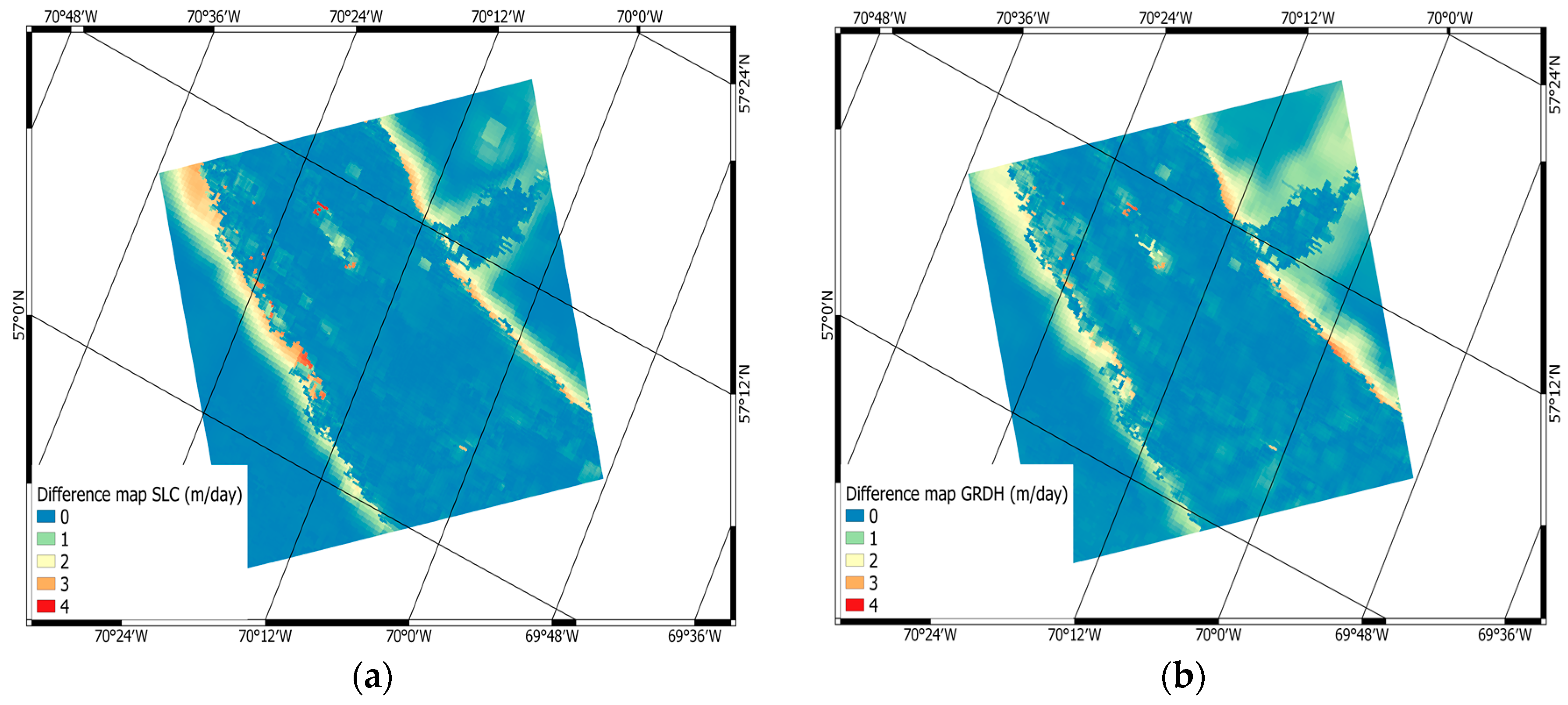
Figure 5.
PG, velocity difference map relevant to the observation period 6–12 January 2017 between the implemented frequency domain OT and reference data for (a) SLC and (b) GRDH image input.
Figure 5.
PG, velocity difference map relevant to the observation period 6–12 January 2017 between the implemented frequency domain OT and reference data for (a) SLC and (b) GRDH image input.
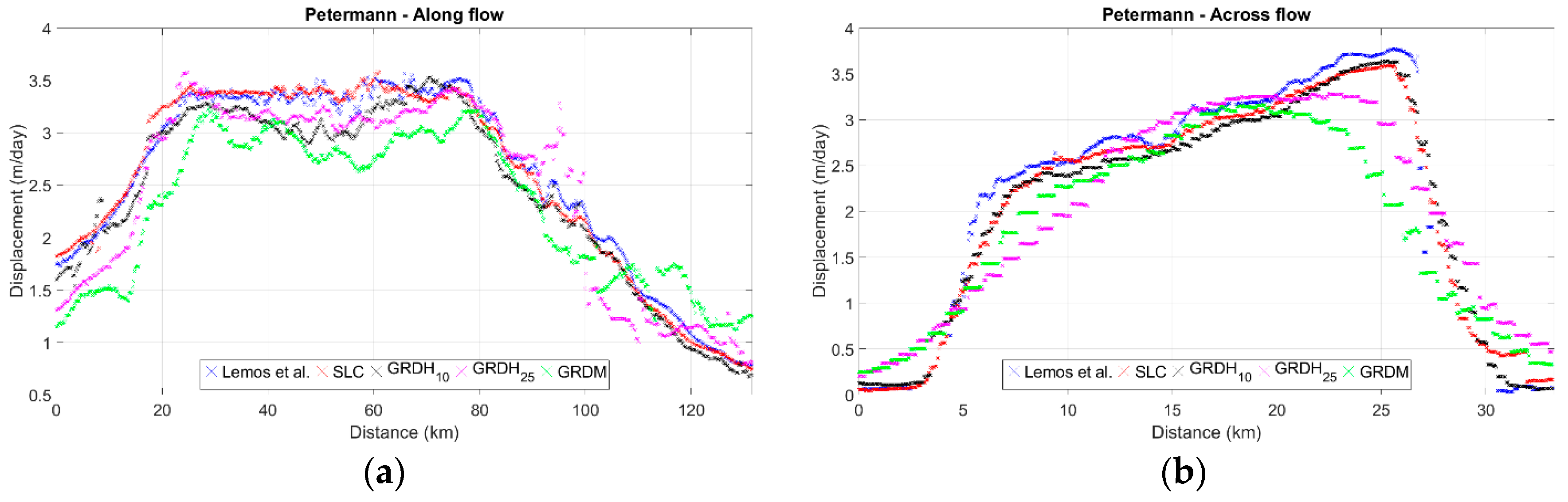
Figure 6.
PG, average annual flow speed for reference data (blue curve) and all the analyzed products (IW SLC red curve, IW GRDH black curve, EW GRDH magenta curve, EW GRDM green curve). (a) Along flow speed. (b) Across flow speed.
Figure 6.
PG, average annual flow speed for reference data (blue curve) and all the analyzed products (IW SLC red curve, IW GRDH black curve, EW GRDH magenta curve, EW GRDM green curve). (a) Along flow speed. (b) Across flow speed.
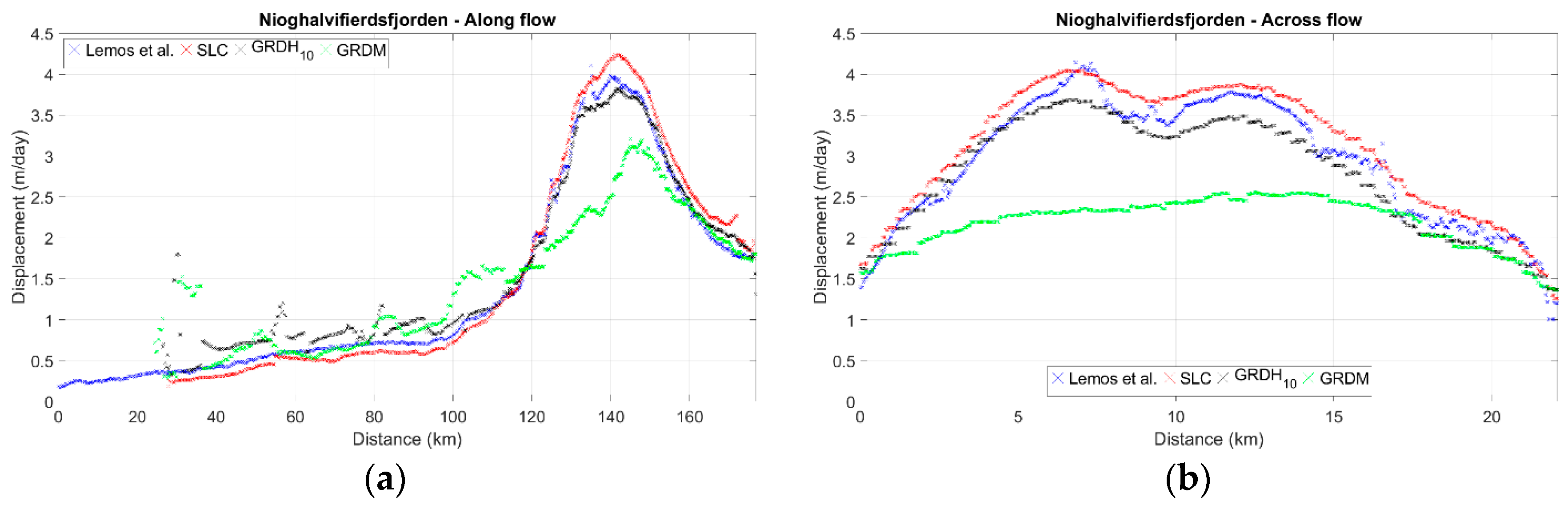
Figure 7.
NI, average annual flow speed for reference data (blue curve) and all the analyzed products (IW SLC red curve, IW GRDH black curve, EW GRDM green curve). (a) Along flow speed. (b) Across flow speed.
Figure 7.
NI, average annual flow speed for reference data (blue curve) and all the analyzed products (IW SLC red curve, IW GRDH black curve, EW GRDM green curve). (a) Along flow speed. (b) Across flow speed.
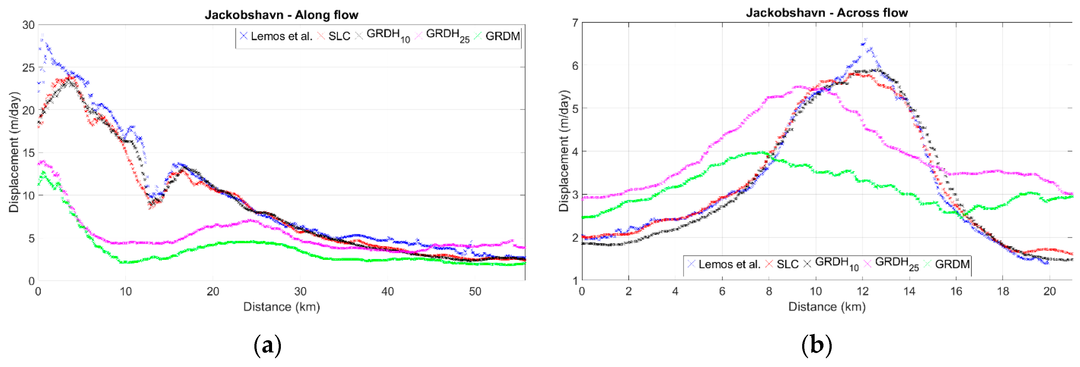
Figure 8.
JAK, average annual flow speed for reference data (blue curve) and all the analyzed products (IW SLC red curve, IW GRDH black curve, EW GRDH magenta curve, EW GRDM green curve). (a) Along flow speed. (b) Across flow speed.
Figure 8.
JAK, average annual flow speed for reference data (blue curve) and all the analyzed products (IW SLC red curve, IW GRDH black curve, EW GRDH magenta curve, EW GRDM green curve). (a) Along flow speed. (b) Across flow speed.
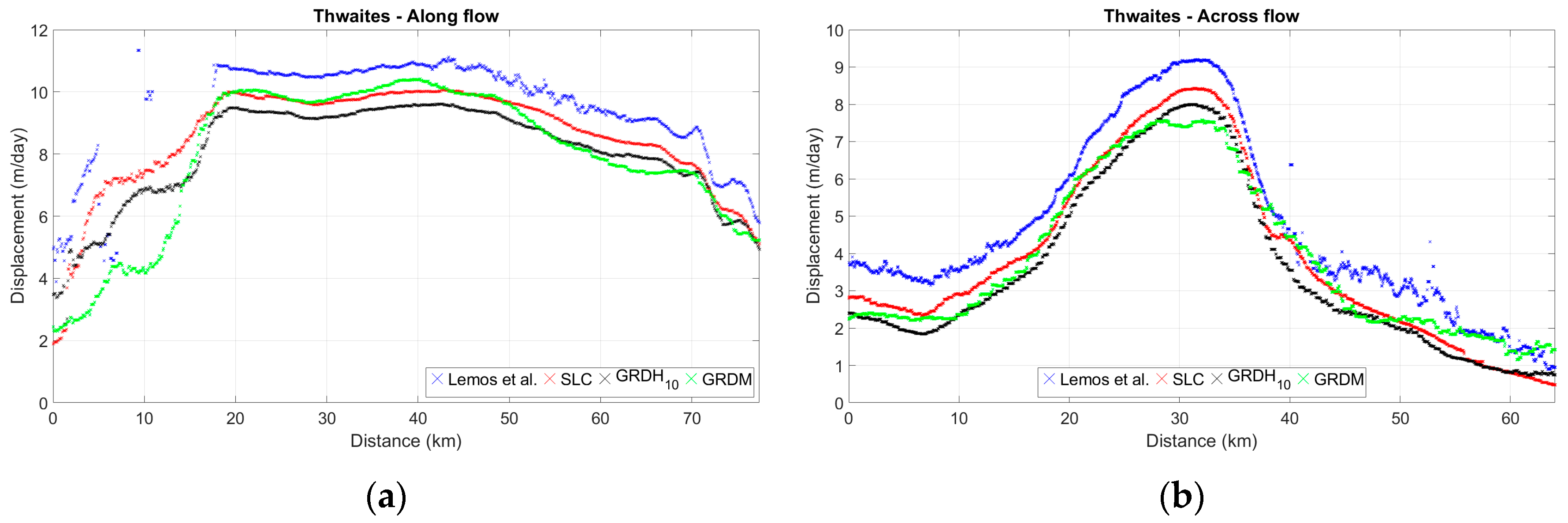
Figure 9.
THW, average annual flow speed for reference data (blue curve) and all the analyzed products (IW SLC red curve, IW GRDH black curve, EW GRDM green curve). (a) Along flow speed. (b) Across flow speed.
Figure 9.
THW, average annual flow speed for reference data (blue curve) and all the analyzed products (IW SLC red curve, IW GRDH black curve, EW GRDM green curve). (a) Along flow speed. (b) Across flow speed.
Table 1.
OT algorithm parameters for the different product classes and test sites.
Table 1.
OT algorithm parameters for the different product classes and test sites.
| Parameter | Unit | SLC | GRDH10 | GRDH25 | GRDM | Glacier |
|---|
Pixel spacing
azimuth/range | m | 13.9/3.79 | 10.1/10.0 | 25.4/25.3 | 40.6/40.4 | PG |
| 13.8/3.49 | 10.1/10.0 | na | 40.5/40.0 | NI |
| 13.8/7.04 | 10.1/10.0 | 25.4/25.3 | 40.6/40.6 | JAK |
| 14.03/4.27 | 10.1/10.0 | na | 40.3/40.1 | THW |
Sensitivity
azimuth/range | m | [0.9, 1.7]/0.9 | [1.2, 2.5]/[1.2, 2.5] | 1.6/1.6 | 2.5/2.5 | PG |
| [0.9, 1.7]/0.9 | [1.2, 2.5]/[1.2, 2.5] | na | 2.5/2.5 | NI |
| 1.7/1.7 | [1.2, 2.5]/[1.2, 2.5] | 1.6/1.6 | 2.5/2.5 | JAK |
| [0.9, 1.7]/0.9 | [1.2, 2.5]/[1.2, 2.5] | na | 2.5/2.5 | THW |
CC window size
azimuth/range | m | [64, 128]/[64, 256] | [64, 256]/[64, 256] | [64, 128]/[64, 128] | [64, 128]/[64, 128] | PG |
| [64, 128]/[64, 256] | [64, 256]/[64, 256] | na | [64, 128]/[64, 128] | NI |
| [64, 128]/[64, 128] | [64, 128]/[64, 128] | [64, 128]/[64, 128] | [64, 128]/[64, 128] | JAK |
| [64, 128]/[64, 256] | [64, 256]/[64, 256] | na | [64, 128]/[64, 128] | THW |
Grid size
azimuth/range | Pixel | 30/100
30/50 (JAK) | 40/40 | 30/30 | 20/20 | |
| CC threshold | | 0.1 | |
| q threshold | | 4 | |
| Max flow speed | m/day | 8 | PG |
| 8 | NI |
| 40 | JAK |
| 20 | THW |
| Subset size | km2 × 103 | 37.8 | 25.0 | 53.8 | 47.4 | PG |
| 21.3 | 15.0 | na | 43.8 | NI |
| 9.65 | 4.43 | 13.42 | 7.22 | JAK |
| 23.5 | 13.6 | na | 22.8 | THW |
Table 2.
Monthly average flow velocities for the four considered glaciers extracted from the reference literature [
47]. Values are expressed in m/day.
Table 2.
Monthly average flow velocities for the four considered glaciers extracted from the reference literature [
47]. Values are expressed in m/day.
| Time | PG | NI | JAK | THW |
|---|
| Along | Across | Along | Across | Along | Across | Along | Across |
|---|
| January | 2.49 | 2.95 | 1.94 | 2.86 | 10.6 | 3.45 | 9.64 | 4.75 |
| February | 2.58 | 2.86 | 1.92 | 2.87 | 9.76 | 3.26 | 9.88 | 5.62 |
| March | 2.57 | 2.87 | 1.93 | 2.90 | 9.71 | 3.30 | 9.86 | 5.26 |
| April | 2.45 | 2.91 | 1.88 | 2.88 | 9.26 | 3.29 | 9.75 | 4.87 |
| May | 2.47 | 2.97 | 1.92 | 2.87 | 10.3 | 2.47 | 9.68 | 5.07 |
| June | 2.60 | 2.99 | 1.89 | 3.04 | 12.3 | 3.17 | 9.64 | 5.20 |
| July | 3.56 | 3.22 | 3.16 | 3.12 | 8.80 | 3.48 | 9.67 | 5.05 |
| August | 2.87 | 3.21 | 1.97 | 3.08 | 13.0 | 3.54 | 9.08 | 5.09 |
| September | 2.69 | 2.96 | 1.90 | 2.99 | 11.0 | 3.25 | 9.08 | 4.68 |
| October | 2.73 | 2.90 | 1.94 | 2.90 | 10.4 | 3.25 | 9.39 | 4.68 |
| November | 2.73 | 2.93 | 1.88 | 2.92 | 10.0 | 3.25 | 9.71 | 4.73 |
| December | 2.72 | 2.93 | 1.93 | 2.91 | 9.65 | 3.24 | 10.3 | 4.75 |
Table 3.
PG, IW SLC product class experiments, RMSE (expressed in m/day) with respect to available literature data measured along selected along flow and across flow transects.
Table 3.
PG, IW SLC product class experiments, RMSE (expressed in m/day) with respect to available literature data measured along selected along flow and across flow transects.
| Petermann–IW SLC |
|---|
| Observation | Track | w = 64, f = 16/4 | w = 64/128, f = 8/4 | w = 128, f = 8/4 | w = 64/256, f = 8/4 |
|---|
| Along | Across | Along | Across | Along | Across | Along | Across |
|---|
| 6–12 Jan | 26 AA | 0.14 | 0.10 | 0.14 | 0.14 | 0.14 | 0.17 | 0.10 | 0.14 |
| 11–17 Feb | 26 DD | 0.30 | 0.26 | 0.28 | 0.28 | 0.28 | 0.28 | 0.28 | 0.26 |
| 1–7 Mar | 26 DD | 0.14 | 0.14 | 0.14 | 0.14 | 0.10 | 0.14 | 0.10 | 0.14 |
| 6–12 Apr | 26 DD | 0.20 | 0.14 | 0.22 | 0.14 | 0.22 | 0.14 | 0.20 | 0.14 |
| 18–24 May | 26 DD | 0.17 | 0.10 | 0.14 | 0.17 | 0.17 | 0.14 | 0.14 | 0.14 |
| 11–17 Jun | 26 DD | 0.14 | 0.10 | 0.28 | 0.24 | 0.17 | 0.35 | 0.20 | 0.28 |
| 11–17 Aug | 26 DD | 0.20 | 0.26 | 0.20 | 0.35 | 0.17 | 0.28 | 0.17 | 0.33 |
| 10–16 Aug | 26 DD | 0.26 | 0.45 | 0.22 | 0.45 | 0.22 | 0.44 | 0.24 | 0.35 |
| 9–15 Sep | 26 DD | 0.10 | 0.10 | 0.10 | 0.10 | 0.00 | 0.10 | 0.10 | 0.10 |
| 9–15 Oct | 26 DD | 0.14 | 0.17 | 0.14 | 0.17 | 0.14 | 0.17 | 0.14 | 0.17 |
| 8–14 Nov | 26 DD | 0.10 | 0.14 | 0.10 | 0.17 | 0.14 | 0.20 | 0.10 | 0.17 |
| 8–14 Dec | 26 DD | 0.24 | 0.32 | 0.26 | 0.35 | 0.24 | 0.35 | 0.26 | 0.36 |
| Time | | ≈1.5 h | ≈1.7 h | ≈3.5 h | ≈4 h |
Table 4.
PG, IW GRDH product class experiments, RMSE (expressed in m/day) with respect to available literature data measured along selected along flow and across flow transects.
Table 4.
PG, IW GRDH product class experiments, RMSE (expressed in m/day) with respect to available literature data measured along selected along flow and across flow transects.
| Petermann–IW GRDH |
|---|
| Observation | Track | w = 64, f = 8 | w = 128, f = 8 | w = 256, f = 4 |
|---|
| Along | Across | Along | Across | Along | Across |
|---|
| 6–12 Jan | 26 AA | 0.17 | 0.24 | 0.14 | 0.17 | 0.14 | 0.32 |
| 11–17 Feb | 26 DD | 0.28 | 0.26 | 0.24 | 0.24 | 0.22 | 0.33 |
| 1–7 Mar | 26 DD | 0.26 | 0.24 | 0.24 | 0.22 | 0.22 | 0.30 |
| 6–12 Apr | 26 DD | 0.28 | 0.28 | 0.24 | 0.28 | 0.22 | 0.48 |
| 18–24 May | 26 DD | 0.28 | 0.32 | 0.26 | 0.30 | 0.17 | 0.45 |
| 11–17 Jun | 26 DD | 0.87 | 0.48 | 0.28 | 0.47 | 0.32 | 0.46 |
| 11–17 Aug | 26 DD | 0.36 | 0.32 | 0.32 | 0.28 | 0.28 | 0.37 |
| 10–16 Aug | 26 DD | 0.24 | 0.24 | 0.22 | 0.20 | 0.20 | 0.30 |
| 9–15 Sep | 26 DD | 0.17 | 0.17 | 0.17 | 0.28 | 0.42 | 0.30 |
| 9–15 Oct | 26 DD | 0.17 | 0.28 | 0.10 | 0.17 | 0.10 | 0.41 |
| 8–14 Nov | 26 DD | 0.24 | 0.20 | 0.24 | 0.20 | 0.14 | 0.33 |
| 8–14 Dec | 26 DD | 0.33 | 0.22 | 0.33 | 0.22 | 0.26 | 0.37 |
| Time | | ≈1 h | ≈7.5 h | ≈8.8 h |
Table 5.
PG, EW GRDH and EW GRDM product classes experiments, RMSE (expressed in m/day) with respect to available literature data measured along selected along flow and across flow transects.
Table 5.
PG, EW GRDH and EW GRDM product classes experiments, RMSE (expressed in m/day) with respect to available literature data measured along selected along flow and across flow transects.
| | Petermann–EW GRDH | Petermann–EW GRDM |
|---|
| Observation | Track | w = 64, f = 16 | w = 128, f = 16 | w = 64, f =16 | w = 128, f = 16 |
|---|
| Along | Across | Along | Across | Along | Across | Along | Across |
|---|
| 1–7 Jan | 41 AA | na | na | na | na | na | na | na | na |
| 12–18 Feb | 41 DD | na | na | na | na | na | na | na | na |
| 8–1 Apr | 41 AA | na | na | na | na | na | na | na | na |
| 1–13 Apr | 41 AA | 0.47 | 0.46 | 0.42 | 0.75 | 0.69 | 0.66 | 0.67 | 1.02 |
| 7–19 May | 41 AA | 0.45 | 0.62 | 0.44 | 0.62 | 0.67 | 0.91 | 0.73 | 1.17 |
| 10–22 Jun | 41 AA | na | na | 0.35 | 0.68 | 0.61 | 0.98 | 0.57 | 1.21 |
| 6–18 Jul | 41 AA | 0.88 | 0.82 | 0.62 | 0.68 | 0.49 | 0.68 | 0.75 | 1.07 |
| 11–23 Aug | 41 AA | 0.50 | 0.59 | 0.37 | 0.63 | 0.48 | 0.59 | 0.69 | 1.10 |
| 4–16 Sep | 41 AA | 0.36 | 0.40 | 0.32 | 0.41 | 0.62 | 0.94 | 0.60 | 1.14 |
| 10–22 Oct | 41 AA | 0.48 | 0.52 | 0.36 | 0.69 | 0.70 | 0.81 | 0.48 | 1.10 |
| 3–15 Nov | 41 AA | 0.33 | 0.35 | 0.35 | 0.45 | 0.71 | 0.71 | 0.42 | 1.07 |
| 9–21 Dec | 41 AA | 0.33 | 0.41 | 0.33 | 0.66 | 0.33 | 0.63 | 0.22 | 1.04 |
| Time | | ≈0.8 h | ≈22.4 h | ≈1.7 h | ≈15.6 h |
Table 6.
NI, IW SLC product class experiments, RMSE (expressed in m/day) with respect to available literature data measured along selected along/across flow transects.
Table 6.
NI, IW SLC product class experiments, RMSE (expressed in m/day) with respect to available literature data measured along selected along/across flow transects.
| Nioghalvifierdsfjorden–IW SLC |
|---|
| Observation | Track | w = 64, f = 16/4 | w = 64/128, f = 8/4 | w = 128, f = 8/4 | w = 256, f = 8/4 |
|---|
| Along | Across | Along | Across | Along | Across | Along | Across |
|---|
| 3–9 Jan | 74 AA | 0.36 | 0.47 | 0.33 | 0.32 | 0.33 | 0.39 | 0.33 | 0.44 |
| 2–8 Feb | 74 AA | 0.24 | 0.20 | 0.30 | 0.26 | 0.30 | 0.24 | 0.30 | 0.30 |
| 4–10 Mar | 74 AA | 0.28 | 0.26 | 0.47 | 0.45 | 0.45 | 0.47 | 0.37 | 0.41 |
| 15–21 Apr | 74 AA | 0.14 | 0.22 | 0.10 | 0.22 | 0.10 | 0.24 | 0.10 | 0.30 |
| 3–9 May | 74 AA | 0.28 | 0.41 | 0.42 | 0.40 | 0.37 | 0.45 | 0.39 | 0.52 |
| 2–8 Jun | 74 AA | 0.52 | 0.59 | 0.70 | 0.66 | 0.49 | 0.48 | 0.49 | 0.53 |
| 2–8 Jul | 74 AA | 0.28 | 0.53 | 1.05 | 1.02 | 0.22 | 0.37 | 0.22 | 0.42 |
| 1–7 Aug | 74 AA | 0.42 | 0.40 | 1.35 | 1.04 | 0.24 | 0.37 | 0.26 | 0.40 |
| 6–12 Sep | 74 AA | 0.33 | 0.32 | 0.32 | 0.33 | 0.28 | 0.20 | 0.56 | 0.28 |
| 6–12 Oct | 74 AA | 0.14 | 0.20 | 0.14 | 0.30 | 0.10 | 0.14 | 0.14 | 0.20 |
| 5–11 Nov | 74 AA | 0.14 | 0.17 | 0.20 | 0.50 | 0.10 | 0.20 | 0.14 | 0.26 |
| 5–11 Dec | 74 AA | 0.14 | 0.22 | 0.22 | 0.17 | 0.22 | 0.20 | 0.22 | 0.17 |
| Time | | ≈1 h | ≈1.4 h | ≈2.8 h | ≈15.8 h |
Table 7.
NI, IW GRDH product class experiments, RMSE (expressed in m/day) with respect to available literature data measured along selected along/across flow transects.
Table 7.
NI, IW GRDH product class experiments, RMSE (expressed in m/day) with respect to available literature data measured along selected along/across flow transects.
| Nioghalvifierdsfjorden–IW GRDH |
|---|
| Observation | Track | w = 64, f = 8 | w = 128, f = 8 | w = 256, f = 4 |
|---|
| Along | Across | Along | Across | Along | Across |
|---|
| 3–9 Jan | 74 AA | 0.24 | 0.33 | 0.22 | 0.32 | 0.17 | 0.26 |
| 2–8 Feb | 74 AA | 0.35 | 0.54 | 0.32 | 0.57 | 0.28 | 0.47 |
| 4–10 Mar | 74 AA | 0.30 | 0.56 | 0.24 | 0.52 | 0.22 | 0.45 |
| 15–21 Apr | 74 AA | 0.28 | 0.48 | 0.24 | 0.48 | 0.20 | 0.42 |
| 3–9 May | 74 AA | 0.24 | 0.33 | 0.24 | 0.33 | 0.24 | 0.39 |
| 2–8 Jun | 74 AA | 0.30 | 0.40 | 0.30 | 0.41 | 0.33 | 0.47 |
| 2–8 Jul | 74 AA | 0.17 | 0.24 | 0.20 | 0.26 | 0.14 | 0.28 |
| 1–7 Aug | 74 AA | 0.20 | 0.44 | 0.14 | 0.30 | 0.20 | 0.37 |
| 6–12 Sep | 74 AA | 0.61 | 0.50 | 0.32 | 0.24 | 0.63 | 0.22 |
| 6–12 Oct | 74 AA | 0.14 | 0.22 | 0.10 | 0.20 | 0.26 | 0.35 |
| 5–11 Nov | 74 AA | 0.10 | 0.10 | 0.10 | 0.36 | 0.22 | 0.36 |
| 5–11 Dec | 74 AA | 0.10 | 0.24 | 0.10 | 0.24 | 0.20 | 0.33 |
| Time | | ≈0.7 h | ≈4.5 h | ≈5.3 h |
Table 8.
JAK, IW SLC product class experiments, RMSE (expressed in m/day) with respect to available literature data measured along selected along/across flow transects.
Table 8.
JAK, IW SLC product class experiments, RMSE (expressed in m/day) with respect to available literature data measured along selected along/across flow transects.
| Jackobshavn–IW SLC |
|---|
| Observation | Track | w = 64, f = 8/4 | w = 64/128, f = 8/4 | w = 128, f = 8/4 | w = 128/256, f = 8/4 |
|---|
| Along | Across | Along | Across | Along | Along | Along | Across |
|---|
| 4–10 Jan | 90 AA | 1.67 | 0.33 | 1.29 | 0.38 | 1.65 | 0.41 | 2.52 | 0.34 |
| 15–21 Feb | 90 AA | 1.57 | 0.31 | 1.35 | 0.22 | 1.44 | 0.26 | 2.15 | 0.22 |
| 5–11 Mar | 90 AA | 1.55 | 0.26 | 1.56 | 0.24 | 1.57 | 0.26 | 1.97 | 0.28 |
| 4–10 Apr | 90 AA | 1.58 | 0.38 | 1.10 | 0.41 | 1.20 | 0.42 | 1.90 | 0.37 |
| 4–10 May | 90 AA | 1.45 | 0.86 | 1.08 | 0.30 | 1.30 | 0.28 | 2.43 | 0.30 |
| 3–9 Jun | 90 AA | 1.59 | 0.47 | 1.22 | 0.26 | 1.83 | 0.26 | 2.97 | 0.24 |
| 2–2 Aug | 90 AA | 1.12 | 0.22 | 1.35 | 0.20 | 1.22 | 0.22 | 2.32 | 0.28 |
| 20–26 Aug | 90 AA | 2.25 | 0.65 | 2.39 | 0.20 | 1.40 | 0.26 | 3.40 | 0.24 |
| 13–19 Sep | 90 AA | 1.32 | 0.66 | 1.44 | 0.30 | 1.80 | 0.34 | 4.01 | 0.36 |
| 7–13 Oct | 90 AA | 1.75 | 0.48 | 1.27 | 0.31 | 1.55 | 0.36 | 2.20 | 0.33 |
| 6–12 Nov | 90 AA | 1.62 | 0.64 | 1.17 | 0.28 | 1.40 | 0.17 | 2.70 | 0.20 |
| 6–12 Dec | 90 AA | 1.88 | 0.55 | 1.51 | 0.24 | 1.63 | 0.26 | 2.35 | 0.28 |
| Time | | ≈0.2 h | ≈0.3 h | ≈0.6 h | ≈1.6 h |
Table 9.
JAK, IW GRDH product class experiments, RMSE (expressed in m/day) with respect to available literature data measured along selected along/across flow transects.
Table 9.
JAK, IW GRDH product class experiments, RMSE (expressed in m/day) with respect to available literature data measured along selected along/across flow transects.
| Jackobshavn–IW GRDH |
|---|
| Observation | Track | w = 64, f = 8 | w = 64/128, f = 8 | w = 128/64, f = 8 | w = 128, f = 8 | w = 256, f = 4 |
|---|
| Along | Across | Along | Across | Along | Across | Along | Across | Along | Across |
|---|
| 4–10 Jan | 90 AA | 1.99 | 0.79 | 2.03 | 0.82 | 1.89 | 0.85 | 1.45 | 0.42 | 3.07 | 0.45 |
| 15–21 Feb | 90 AA | 1.44 | 0.24 | 1.82 | 0.26 | 1.27 | 0.24 | 1.42 | 0.24 | 2.46 | 0.49 |
| 5–11 Mar | 90 AA | 1.57 | 0.53 | 1.76 | 0.32 | 1.35 | 0.35 | 1.43 | 0.32 | 2.24 | 0.55 |
| 4–10 Apr | 90 AA | 1.81 | 0.77 | 1.37 | 0.37 | 1.17 | 0.40 | 1.10 | 0.35 | 1.98 | 0.49 |
| 4–10 May | 90 AA | 1.61 | 0.41 | 1.79 | 0.41 | 1.28 | 0.42 | 1.76 | 0.44 | 3.08 | 0.42 |
| 3–9 Jun | 90 AA | 1.52 | 0.79 | 1.69 | 0.39 | 1.06 | 0.45 | 1.24 | 0.36 | 3.42 | 0.41 |
| 27–2 Aug | 90 AA | 1.66 | 1.10 | 1.09 | 0.57 | 0.85 | 0.37 | 0.89 | 0.33 | 2.47 | 0.45 |
| 20–26 Aug | 90 AA | 1.86 | 0.58 | 1.88 | 0.57 | 1.20 | 0.37 | 1.17 | 0.28 | 2.91 | 0.32 |
| 13–19 Sep | 90 AA | 2.14 | 0.92 | 1.65 | 0.48 | 1.30 | 0.45 | 1.57 | 0.45 | 3.95 | 0.47 |
| 7–13 Oct | 90 AA | 1.82 | 0.91 | 1.57 | 0.20 | 1.29 | 0.20 | 1.31 | 0.17 | 2.63 | 0.42 |
| 6–12 Nov | 90 AA | 1.97 | 0.71 | 2.20 | 0.70 | 1.72 | 0.63 | 1.35 | 0.44 | 3.24 | 0.33 |
| 6–12 Dec | 90 AA | 1.94 | 0.72 | 1.90 | 0.36 | 1.51 | 0.35 | 1.55 | 0.35 | 2.80 | 0.37 |
| Time | | ≈0.2 h | ≈0.4 h | ≈0.4 h | ≈1.3 h | ≈1.2 h |
Table 10.
THW, IW SLC product class experiments, RMSE (expressed in m/day) with respect to available literature data measured along selected along/across flow transects.
Table 10.
THW, IW SLC product class experiments, RMSE (expressed in m/day) with respect to available literature data measured along selected along/across flow transects.
| Thwaites–IW SLC |
|---|
| Observation | Track | w = 64, f = 16/4 | w = 64/128, f = 16/4 | w = 128, f = 8/4 | w = 128/256, f = 8/4 |
|---|
| Along | Across | Along | Across | Along | Across | Along | Across |
|---|
| 9–15 Jan | 65 AA | 0.62 | 0.62 | 0.67 | 0.70 | 0.73 | 0.74 | 0.71 | 0.73 |
| 20–26 Feb | 65 AA | na | na | na | na | na | na | na | na |
| 10–16 Mar | 65 AA | na | na | na | na | na | na | na | na |
| 9–15 Apr | 65 AA | 0.51 | 0.52 | 0.48 | 0.50 | 0.50 | 0.49 | 0.47 | 0.49 |
| 15–21 May | 65 AA | 1.79 | 1.56 | 1.78 | 1.61 | 1.68 | 1.52 | 1.65 | 1.52 |
| 2–8 Jun | 65 AA | 1.17 | 1.28 | 1.13 | 1.37 | 1.11 | 1.34 | 1.08 | 1.35 |
| 2–8 Jul | 65 DD | 1.10 | 1.15 | 0.98 | 1.09 | 0.89 | 1.05 | 0.89 | 1.05 |
| 1–7 Aug | 65 DD | na | Na | na | na | na | na | na | na |
| 6–12 Sep | 65 DD | 1.64 | 1.10 | 1.75 | 1.27 | 1.77 | 1.25 | 1.65 | 1.09 |
| 6–12 Oct | 65 DD | 0.71 | 0.59 | 0.61 | 0.53 | 0.66 | 0.56 | 0.66 | 0.55 |
| 5–11 Nov | 65 DD | 0.99 | 0.68 | 0.94 | 0.63 | 0.96 | 0.69 | 0.78 | 0.59 |
| 5–11 Dec | 65 DD | 1.68 | 0.83 | 1.37 | 0.95 | 1.42 | 1.00 | 1.52 | 0.98 |
| Time | | ≈0.75 h | ≈1.5 h | ≈2 h | ≈4.9 h |
Table 11.
THW, IW GRDH product class experiments, RMSE (expressed in m/day) with respect to available literature data measured along selected along/across flow transects.
Table 11.
THW, IW GRDH product class experiments, RMSE (expressed in m/day) with respect to available literature data measured along selected along/across flow transects.
| Thwaites–IW GRDH |
|---|
| Observation | Track | w = 64, f = 8 | w = 128, f = 8 | w = 256, f = 4 |
|---|
| Along | Across | Along | Across | Along | Across |
|---|
| 9–15 Jan | 65 AA | 0.95 | 0.90 | 0.84 | 0.87 | 1.07 | 1.00 |
| 20–26 Feb | 65 AA | na | na | 1.64 | 1.51 | 1.71 | 1.51 |
| 10–16 Mar | 65 AA | na | na | na | na | 1.29 | 1.27 |
| 9–15 Apr | 65 AA | 1.55 | 1.20 | 1.41 | 1.21 | 1.47 | 1.26 |
| 15–21 May | 65 AA | 1.55 | 1.28 | 1.70 | 1.45 | 1.49 | 1.30 |
| 2–8 Jun | 65 AA | 1.52 | 1.51 | 1.55 | 1.47 | 1.45 | 1.39 |
| 2–8 Jul | 65 DD | 1.33 | 0.99 | 1.43 | 1.31 | 0.84 | 0.73 |
| 1–7 Aug | 65 DD | na | na | na | na | 1.38 | 1.26 |
| 6–12 Sep | 65 DD | 1.97 | 1.70 | 2.01 | 1.67 | 2.12 | 1.72 |
| 6–12 Oct | 65 DD | 1.28 | 1.28 | 1.20 | 1.20 | 1.26 | 1.23 |
| 5–11 Nov | 65 DD | na | na | 1.16 | 1.36 | 1.42 | 1.49 |
| 5–11 Dec | 65 DD | 1.49 | 1.43 | 1.57 | 1.56 | 1.73 | 1.36 |
| Time | | ≈0.5 h | ≈2.5 h | ≈3.5 h |
Table 12.
RMSE (expressed in m/day) against reference literature for the selected along/across flow transects for the four analyzed glaciers and product classes calculated by averaging one year of observations.
Table 12.
RMSE (expressed in m/day) against reference literature for the selected along/across flow transects for the four analyzed glaciers and product classes calculated by averaging one year of observations.
| Glacier | IW SLC | IW GRDH | EW GRDH | EW GRDM |
|---|
| | Along | Across | Along | Across | Along | Across | Along | Across |
|---|
| Petermann | 0.10 | 0.20 | 0.17 | 0.24 | 0.32 | 0.50 | 0.53 | 0.66 |
| Nioghalvifierdsfjorden | 0.17 | 0.20 | 0.14 | 0.20 | na | na | 0.57 | 0.91 |
| Jackobshavn | 1.69 | 0.17 | 1.55 | 0.22 | 7.37 | 1.24 | 8.39 | 1.37 |
| Thwaites | 1.10 | 0.81 | 1.41 | 1.17 | na | na | 1.63 | 1.01 |
Table 13.
RMSE (expressed in m/day) for the displacement velocities calculated with the in-house OT algorithm with respect to reference IW SLC results for the PG (left panel) and NI (right panel).
Table 13.
RMSE (expressed in m/day) for the displacement velocities calculated with the in-house OT algorithm with respect to reference IW SLC results for the PG (left panel) and NI (right panel).
| Petermann | Nioghalvifierdsfjorden |
|---|
| Observation | Track | IW GRDH | Observation | Track | IW GRDH |
|---|
| Along | Across | Along | Across |
|---|
| 6–12 Jan | 26 AA | 0.17 | 0.36 | 3–9 Jan | 74 AA | 0.47 | 0.39 |
| 11–17 Feb | 26 DD | 0.26 | 0.20 | 2–8 Feb | 74 AA | 0.47 | 0.59 |
| 1–7 Mar | 26 DD | 0.32 | 0.30 | 4–10 mar | 74 AA | 0.42 | 0.49 |
| 6–12 Apr | 26 DD | 0.26 | 0.35 | 15–21 Apr | 74 AA | 0.30 | 0.54 |
| 18–24 May | 26 DD | 0.36 | 0.30 | 3–9 May | 74 AA | 0.30 | 0.67 |
| 11–17 Jun | 26 DD | 0.44 | 0.92 | 2–8 Jun | 74 AA | 0.46 | 0.66 |
| 11–17 Jul | 26 DD | 0.35 | 0.73 | 2–8 Jul | 74 AA | 0.28 | 0.30 |
| 10–16 Aug | 26 DD | 0.26 | 0.69 | 1–7 Aug | 74 AA | 0.54 | 0.30 |
| 9–15 Sep | 26 DD | 0.20 | 0.20 | 6–12 Sep | 74 AA | 0.64 | 0.32 |
| 9–15 Oct | 26 DD | 0.14 | 0.22 | 6–12 Oct | 74 AA | 0.17 | 0.24 |
| 8–14 Nov | 26 DD | 0.22 | 0.14 | 5–11 Nov | 74 AA | 0.20 | 0.36 |
| 8–14 Dec | 26 DD | 0.33 | 0.17 | 5–11 Dec | 74 AA | 0.26 | 0.20 |
| Mean | | 0.20 | 0.10 | Mean | | 0.24 | 0.33 |
Table 14.
RMSE (expressed in m/day) for the displacement velocities calculated with the in-house OT algorithm with respect to reference IW SLC results for JAK (left panel) and THW (right panel).
Table 14.
RMSE (expressed in m/day) for the displacement velocities calculated with the in-house OT algorithm with respect to reference IW SLC results for JAK (left panel) and THW (right panel).
| Jackobshavn | Thwaites |
|---|
| Observation | Track | GRDH10 | Observation | Track | GRDH10 |
|---|
| Along | Across | Along | Across |
|---|
| 4–10 Jan | 90 AA | 1.36 | 0.75 | 9–15 Jan | 65 AA | 0.62 | 0.33 |
| 15–21 Feb | 90 AA | 1.19 | 0.20 | 20–26 Feb | 65 AA | na | na |
| 5–11 Mar | 90 AA | 1.23 | 0.32 | 10–16 Mar | 65 AA | na | na |
| 4–10 Apr | 90 AA | 1.79 | 0.30 | 9–15 Apr | 65 AA | 1.12 | 1.18 |
| 4–10 May | 90 AA | 0.95 | 0.42 | 15–21 May | 65 AA | 0.62 | 0.30 |
| 3–9 Jun | 90 AA | 0.95 | 0.56 | 2–8 Jun | 65 AA | 0.64 | 0.24 |
| 27–2 Aug | 90 AA | 1.34 | 0.40 | 2–8 Jul | 65 DD | 0.79 | 0.47 |
| 20–26 Aug | 90 AA | 2.36 | 0.42 | 1–7 Aug | 65 DD | na | na |
| 13–19 Sep | 90 AA | 1.38 | 0.36 | 6–12 Sep | 65 DD | 0.57 | 0.69 |
| 7–13 Oct | 90 AA | 1.24 | 0.35 | 6–12 Oct | 65 DD | 0.74 | 0.85 |
| 6–12 Nov | 90 AA | 1.18 | 0.73 | 5–11 Nov | 65 DD | 0.92 | 1.04 |
| 6–12 Dec | 90 AA | 0.90 | 0.26 | 5–11 Dec | 65 DD | 0.72 | 0.45 |
| Mean | | 0.67 | 0.17 | Mean | | 0.75 | 0.45 |
Table 15.
Storage needs (in GB) per analyzed time-series, processing step, and product class.
Table 15.
Storage needs (in GB) per analyzed time-series, processing step, and product class.
| Glacier | Level-1 | Coregistration | Subset | OT | Map | Product |
|---|
| PG | 93.1 | 78.8 | 62.5 | 62.5 | 0.35 | IW SLC |
| 20.2 | 37.8 | 22.0 | 22.0 | 0.24 | IW GRDH |
| 15.2 | 18.2 | 5.66 | 5.66 | 0.77 | EW GRDH |
| 5.74 | 8.92 | 1.95 | 1.95 | 0.67 | EW GRDM |
| NI | 106 | 81.6 | 39.4 | 39.4 | 0.20 | IW SLC |
| 22.9 | 37.8 | 13.2 | 13.2 | 0.15 | IW GRDH |
| 6.07 | 8.66 | 2.21 | 2.21 | 0.27 | EW GRDM |
| JAK | 80.5 | 80.2 | 17.7 | 17.7 | 0.07 | IW SLC |
| 17.7 | 38.3 | 3.91 | 3.91 | 0.04 | IW GRDH |
| 17.6 | 19.2 | 1.70 | 1.70 | 0.17 | EW GRDH |
| 6.54 | 9.30 | 0.45 | 0.45 | 0.11 | EW GRDM |
| THW | 51.6 | 77.3 | 36.7 | 36.7 | 0.28 | IW SLC |
| 12.0 | 37.9 | 11.3 | 11.3 | 0.12 | IW GRDH |
| 6.40 | 9.28 | 1.28 | 1.28 | 0.20 | EW GRDM |


