Comparison of Hyperspectral Techniques for Urban Tree Diversity Classification

 ,
,
Abstract
:
1. Introduction
- Feature extraction is defined as a set of methods for extracting information from an image [33], such as transformative methods to derive a characteristic [34]. Principal component analysis (PCA) is often used as a DR method because it preserves the greatest spectral variability of original images [35]. However, it does not take account of the signal-to-noise ratio (SNR), unlike the minimal noise fraction (MNF) [36].
- Feature selection methods consist of considering one or more subsets of initial features according to their relevance to the considered question. These methods preserve the interpretability of the original data [37]. In the absence of prior knowledge, a selection is made based on the most informative, least correlated elements in order to preserve the original information as much as possible [38,39]. Vegetation indices are regularly used to provide information on the biogeochemical properties of plants in order to distinguish them. Moreover, these indices allow for better discrimination than when using spectral values from spectral bands alone, for instance in the case of a vegetation class whose composition is too similar [37].
2. Materials and Methods
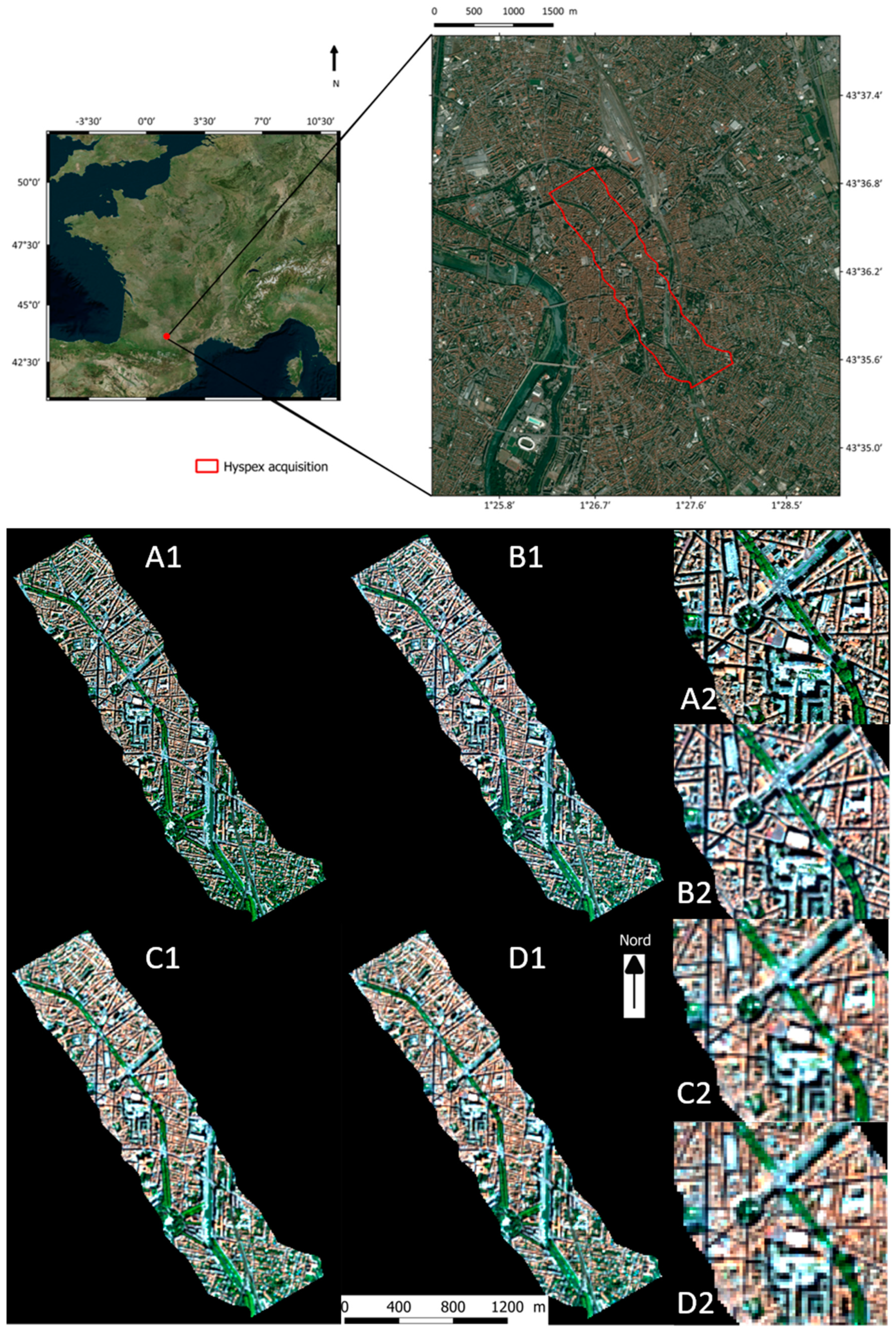
2.1. Study Area
2.2. Remote Sensing Data
2.3. In Situ Samples
2.4. Methods
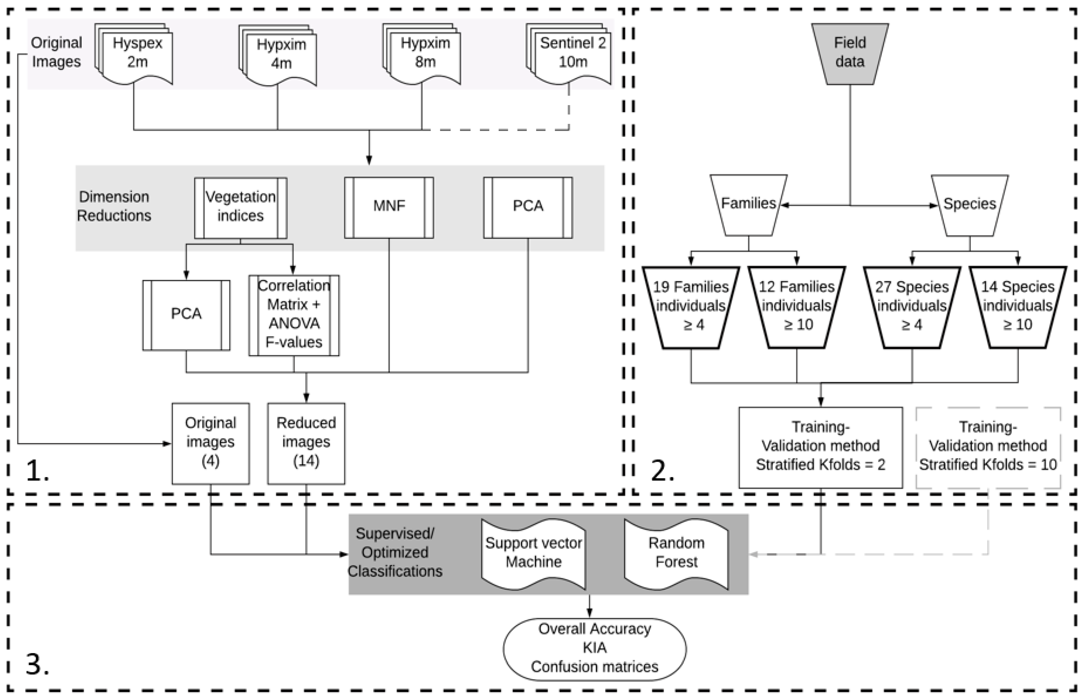
2.4.1. Overall Approach
2.4.2. Dimension Reductions Methods
- The K-best method uses the F-value of ANOVA (analysis of variance) as a ranking criterion. It compares the interclass and intra-class dispersion between VI. Subsequently, from a correlation matrix (Pearson’s r), if the correlation between two VI is greater than 85% (r > 0.85) then the VI with the smallest F-value is removed from the selection.
- A PCA method is used to eliminate the correlation between VI. Kaiser’s criterion [39] is used for the selection: components with a eigenvalue greater than 1 represents the same amount of information as a single variable.
2.4.3. Training Datasets and Method
2.4.4. Classification Methods
2.4.5. Experiments: Assessing the Respective and Combined Influence of Hyperspectral Techniques and Data
3. Results
3.1. Dimension Reductions: Comparison of Extracted Components
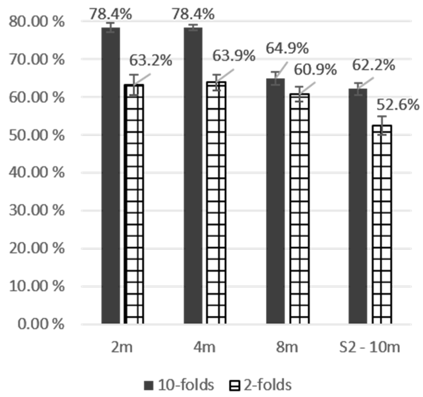
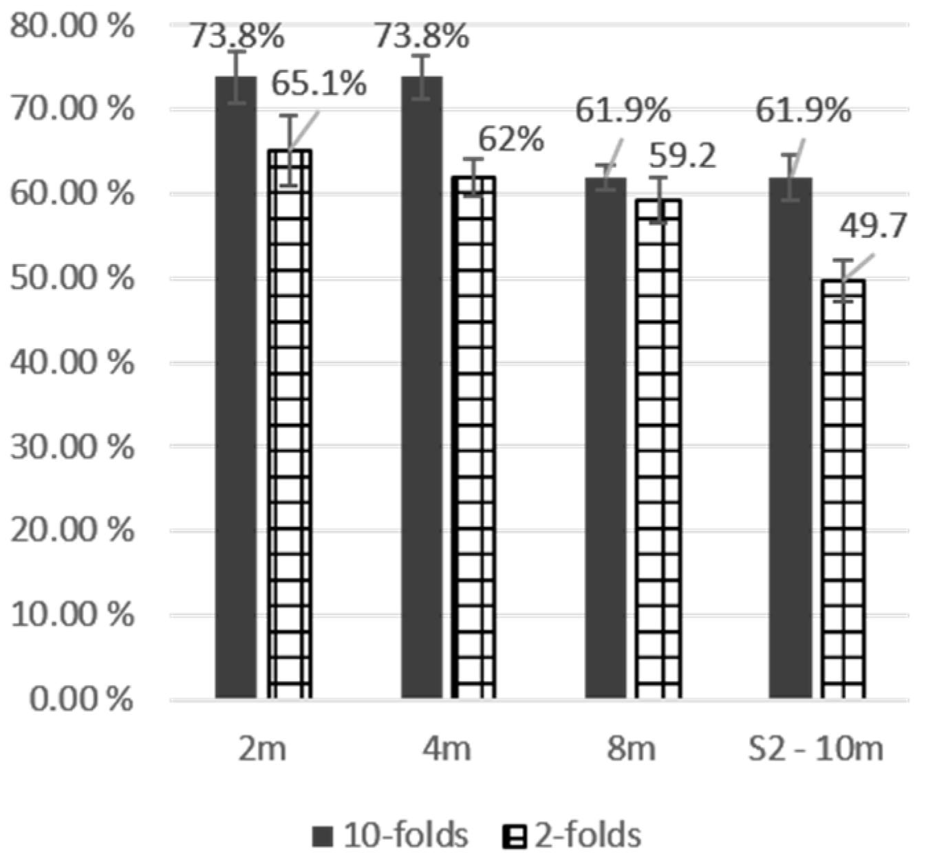
3.2. Evaluation of the Respective Influence of Hyperspectral Techniques and Data
3.3. Influence of Combined Techniques According to Images
4. Discussion
4.1. Evaluating the Respective Influence of Hyperspectral Techniques
4.2. Characterizing Urban Tree Diversity with VHRS Hyperspectral Remote Sensing: Advantages, Limitations and Prospects
4.3. Towards an Urban Sampling Strategy for Mapping Urban Tree Diversity?
5. Conclusions
Supplementary Materials
Author Contributions
Funding
Acknowledgments
Conflicts of Interest
References
- Masson, V.; Marchadier, C.; Adolphe, L.; Aguejdad, R.; Avner, P.; Bonhomme, M.; Bretagne, G.; Briottet, X.; Bueno, B.; de Munck, C.; et al. Adapting cities to climate change: A systemic modelling approach. Urban Clim. 2014, 10, 407–429. [Google Scholar] [CrossRef]
- Alberti, M. The Effects of Urban Patterns on Ecosystem Function. Int. Reg. Sci. Rev. 2005, 28, 168–192. [Google Scholar] [CrossRef]
- El Araby, M. Urban growth and environmental degradation. Cities 2002, 19, 389–400. [Google Scholar] [CrossRef]
- Pickett, S.T.; Burch, W.R., Jr.; Dalton, S.E.; Foresman, T.W.; Grove, J.M.; Rowntree, R. A conceptual framework for the study of human ecosystems in urban areas. Urban Ecosyst. 1997, 185–199. [Google Scholar] [CrossRef]
- Shepherd, J.M. A Review of Current Investigations of Urban-Induced Rainfall and Recommendations for the Future. Earth Interact. 2005, 9, 1–27. [Google Scholar] [CrossRef] [Green Version]
- Escobedo, F.J.; Nowak, D.J. Spatial heterogeneity and air pollution removal by an urban forest. Landsc. Urban Plan. 2009, 90, 102–110. [Google Scholar] [CrossRef]
- Akbari, H.; Pomerantz, M.; Taha, H. Cool surfaces and shade trees to reduce energy use and improve air quality in urban areas. Sol. Energy 2001, 70, 295–310. [Google Scholar] [CrossRef]
- Bolund, P.; Hunhammar, S. Ecosystem services in urban areas. Ecol. Econ. 1999, 29, 293–301. [Google Scholar] [CrossRef]
- Santamouris, M. Using cool pavements as a mitigation strategy to fight urban heat island—A review of the actual developments. Renew. Sustain. Energy Rev. 2013, 26, 224–240. [Google Scholar] [CrossRef]
- McCarthy, H.R.; Pataki, D.E. Drivers of variability in water use of native and non-native urban trees in the greater Los Angeles area. Urban Ecosyst. 2010, 13, 393–414. [Google Scholar] [CrossRef] [Green Version]
- McPherson, E.G.; Simpson, J.R.; Xiao, Q.; Wu, C. Million trees Los Angeles canopy cover and benefit assessment. Landsc. Urban Plan. 2011, 99, 40–50. [Google Scholar] [CrossRef]
- Simpson, J.R. Improved estimates of tree-shade effects on residential energy use. Energy Build. 2002, 34, 1067–1076. [Google Scholar] [CrossRef]
- Lemonsu, A.; Masson, V.; Shashua-Bar, L.; Erell, E.; Pearlmutter, D. Inclusion of vegetation in the Town Energy Balance model for modelling urban green areas. Geosci. Model Dev. 2012, 5, 1377–1393. [Google Scholar] [CrossRef] [Green Version]
- Redon, E.C.; Lemonsu, A.; Masson, V.; Morille, B.; Musy, M. Implementation of street trees within the solar radiative exchange parameterization of TEB in SURFEX v8.0. Geosci. Model Dev. 2017, 10, 385–411. [Google Scholar] [CrossRef] [Green Version]
- Pu, R.; Landry, S.; Yu, Q. Assessing the potential of multi-seasonal high resolution Pléiades satellite imagery for mapping urban tree species. Int. J. Appl. Earth Obs. Geoinf. 2018, 71, 144–158. [Google Scholar] [CrossRef]
- Pu, R.; Landry, S. A comparative analysis of high spatial resolution IKONOS and WorldView-2 imagery for mapping urban tree species. Remote Sens. Environ. 2012, 124, 516–533. [Google Scholar] [CrossRef]
- Alonzo, M.; Bookhagen, B.; Roberts, D.A. Urban tree species mapping using hyperspectral and lidar data fusion. Remote Sens. Environ. 2014, 148, 70–83. [Google Scholar] [CrossRef]
- Voss, M.; Sugumaran, R. Seasonal Effect on Tree Species Classification in an Urban Environment Using Hyperspectral Data, LiDAR, and an Object-Oriented Approach. Sensors 2008, 8, 3020–3036. [Google Scholar] [CrossRef] [PubMed]
- Xiao, Q.; Ustin, S.L.; McPherson, E.G. Using AVIRIS data and multiple-masking techniques to map urban forest tree species. Int. J. Remote Sens. 2004, 25, 5637–5654. [Google Scholar] [CrossRef] [Green Version]
- Boschetti, M.; Boschetti, L.; Oliveri, S.; Casati, L.; Canova, I. Tree species mapping with Airborne hyper-spectral MIVIS data: the Ticino Park study case. Int. J. Remote Sens. 2007, 28, 1251–1261. [Google Scholar] [CrossRef]
- Maschler, J.; Atzberger, C.; Immitzer, M. Individual Tree Crown Segmentation and Classification of 13 Tree Species Using Airborne Hyperspectral Data. Remote Sens. 2018, 10, 1218. [Google Scholar] [CrossRef]
- Immitzer, M.; Vuolo, F.; Atzberger, C. First Experience with Sentinel-2 Data for Crop and Tree Species Classifications in Central Europe. Remote Sens. 2016, 8, 166. [Google Scholar] [CrossRef]
- Gaia Vaglio, L.; Pulleti, N.; Hawthorne, W.; Liesenberg, V.; Corona, P.; Papale, D.; Chen, Q.; Valentini, R. Discrimination of tropical forest types, dominant species, and mapping of functional guilds by hyperspectral and simulated multispectral Sentinel-2 data. Remote Sens. Environ. 2016, 176, 163–176. [Google Scholar] [CrossRef] [Green Version]
- Shi, Y.; Skidmore, A.K.; Wang, T.; Holzwarth, S.; Heiden, U.; Pinnel, N.; Zhu, X.; Heurich, M. Tree species classification using plant functional traits from LiDAR and hyperspectral data. Int. J. Appl. Earth Obs. Geoinf. 2018, 73, 207–219. [Google Scholar] [CrossRef]
- Mozgeris, G.; Juodkienė, V.; Jonikavičius, D.; Straigytė, L.; Gadal, S.; Ouerghemmi, W. Ultra-Light Aircraft-Based Hyperspectral and Colour-Infrared Imaging to Identify Deciduous Tree Species in an Urban Environment. Remote Sens. 2018, 10, 1668. [Google Scholar] [CrossRef]
- Dabiri, Z.; Lang, S. Comparison of Independent Component Analysis, Principal Component Analysis, and Minimum Noise Fraction Transformation for Tree Species Classification Using APEX Hyperspectral Imagery. ISPRS Int. J. Geo Inf. 2018, 7, 488. [Google Scholar] [CrossRef]
- Liu, H.; Wu, C. Crown-level tree species classification from AISA hyperspectral imagery using an innovative pixel-weighting approach. Int. J. Appl. Earth Obs. Geoinf. 2018, 68, 298–307. [Google Scholar] [CrossRef]
- Dalponte, M.; Bruzzone, L.; Vescovo, L.; Gianelle, D. The role of spectral resolution and classifier complexity in the analysis of hyperspectral images of forest areas. Remote Sens. Environ. 2009, 113, 2345–2355. [Google Scholar] [CrossRef]
- Noyel, G. Filtrage, Réduction de Dimension, Classification et Segmentation Morphologique Hyperspectrale. Ph.D. Thesis, Mines ParisTech, University PSL, Paris, France, 2008; 280p. [Google Scholar]
- Landgrebe, D.A. Signal Theory Methods in Multispectral Remote Sensing; John Wiley & Sons: Hoboken, NJ, USA, 2005; Volume 29, ISBN 978-0-471-72125-3. [Google Scholar]
- Lu, D.; Weng, Q. A survey of image classification methods and techniques for improving classification performance. Int. J. Remote Sens. 2007, 28, 823–870. [Google Scholar] [CrossRef]
- Melgani, F.; Bruzzone, L. Classification of hyperspectral remote sensing images with support vector machines. IEEE Trans. Geosci. Remote Sens. 2004, 42, 1778–1790. [Google Scholar] [CrossRef] [Green Version]
- Girard, M.-C.; Girard, C.M. Traitement des Données de Télédétection: Environnement et Ressources Naturelles, 2nd ed.; Technique et Ingénierie; Dunod: Paris, France, 2017; ISBN 2-10-076370-9. [Google Scholar]
- Khoder, J.; Younes, R. Dimensionality reduction on hyperspectral images: A comparative review based on artificial datas. In Proceedings of the 4th International Congress on Image and Signal Processing, Shanghai, China, 15–17 October 2011; pp. 1875–1883. [Google Scholar]
- Farrell, M.D.; Mersereau, R.M. On the Impact of PCA Dimension Reduction for Hyperspectral Detection of Difficult Targets. IEEE Geosci. Remote Sens. Lett. 2005, 2, 192–195. [Google Scholar] [CrossRef]
- Green, A.A.; Berman, M.; Switzer, P. A Transformation for Ordering Multispectral Data in Terms of Image Quality with Implications for Noise Removal. IEEE Trans. Geosci. Remote Sens. 1988, 26, 65–74. [Google Scholar] [CrossRef]
- Erudel, T.; Fabre, S.; Houet, T.; Mazier, F.; Briottet, X. Criteria Comparison for Classifying Peatland Vegetation Types Using In Situ Hyperspectral Measurements. Remote Sens. 2017, 9, 748. [Google Scholar] [CrossRef]
- Clark, M.; Roberts, D.; Clark, D. Hyperspectral discrimination of tropical rain forest tree species at leaf to crown scales. Remote Sens. Environ. 2005, 96, 375–398. [Google Scholar] [CrossRef]
- Kaiser, H.F. The Application of Electronic Computers to Factor Analysis. Educ. Psychol. Meas. 1960, 20, 141–151. [Google Scholar] [CrossRef]
- Becker, B.L.; Lusch, D.P.; Qi, J. A classification-based assessment of the optimal spectral and spatial resolutions for Great Lakes coastal wetland imagery. Remote Sens. Environ. 2007, 108, 111–120. [Google Scholar] [CrossRef]
- Camps-Valls, G.; Bruzzone, L. Kernel Methods for Remote Sensing Data Analysis; Wiley: Hoboken, NJ, USA, 2009; p. 15. [Google Scholar]
- Chan, J.C.-W.; Paelinckx, D. Evaluation of Random Forest and Adaboost tree-based ensemble classification and spectral band selection for ecotope mapping using airborne hyperspectral imagery. Remote Sens. Environ. 2008, 112, 2999–3011. [Google Scholar] [CrossRef]
- Dalponte, M.; Orka, H.O.; Gobakken, T.; Gianelle, D.; Naesset, E. Tree Species Classification in Boreal Forests with Hyperspectral Data. IEEE Trans. Geosci. Remote Sens. 2013, 51, 2632–2645. [Google Scholar] [CrossRef]
- Foody, G.M.; Mathur, A. Toward intelligent training of supervised image classifications: Directing training data acquisition for SVM classification. Remote Sens. Environ. 2004, 93, 107–117. [Google Scholar] [CrossRef]
- Plaza, A.; Benediktsson, J.A.; Boardman, J.W.; Brazile, J.; Bruzzone, L.; Camps-Valls, G.; Chanussot, J.; Fauvel, M.; Gamba, P.; Gualtieri, A.; et al. Recent advances in techniques for hyperspectral image processing. Remote Sens. Environ. 2009, 113, S110–S122. [Google Scholar] [CrossRef]
- Willis, C.J. Hyperspectral Image Classification with Limited Training Data Samples Using Feature Subspaces. In Algorithms and Technologies for Multispectral, Hyperspectral, and Ultraspectral Imagery X; Shen, S.S., Lewis, P.E., Eds.; SPIE: Bellingham, WA, USA, 2004; p. 170. [Google Scholar]
- Rodriguez, J.D.; Perez, A.; Lozano, J.A. Sensitivity Analysis of k-Fold Cross Validation in Prediction Error Estimation. IEEE Trans. Pattern Anal. Mach. Intell. 2010, 32, 569–575. [Google Scholar] [CrossRef] [PubMed]
- Alonzo, M.; Roth, K.; Roberts, D. Identifying Santa Barbara’s urban tree species from AVIRIS imagery using canonical discriminant analysis. Remote Sens. Lett. 2013, 4, 513–521. [Google Scholar] [CrossRef]
- Karoui, M.; Benhalouche, F.; Deville, Y.; Djerriri, K.; Briottet, X.; Le Bris, A. Detection and area estimation for photovoltaic panels in urban hyperspectral remote sensing data by an original NMF-based unmixing method. In Proceedings of the IEEE International Geoscience and Remote Sensing Symposium (IGARSS 2018), Valencia, Spain, 22–27 July 2018. [Google Scholar]
- Miesch, C.; Poutier, L.; Achard, V.; Briottet, X.; Lenot, X.; Boucher, Y. Direct and Inverse Radiative Transfer Solutions for Visible and Near-Infrared Hyperspectral Imagery. IEEE Trans. Geosci. Remote Sens. 2005, 43, 1552–1562. [Google Scholar] [CrossRef]
- Roussel, G.; Weber, C.; Briottet, X.; Ceamanos, X. Comparison of two atmospheric correction methods for the classification of spaceborne urban hyperspectral data depending on the spatial resolution. Int. J. Remote Sens. 2017, 39, 1593–1614. [Google Scholar] [CrossRef]
- Crawford, M.M.; Ham, J.; Chen, Y.; Ghosh, J. Random forests of binary hierarchical classifiers for analysis of hyperspectral data. In Proceedings of the IEEE Workshop on Advances in Techniques for Analysis of Remotely Sensed Data, Greenbelt, MD, USA, 27–28 October 2003; pp. 337–345. [Google Scholar]
- Ham, J.; Chen, Y.; Crawford, M.M.; Ghosh, J. Investigation of the random forest framework for classification of hyperspectral data. IEEE Trans. Geosci. Remote Sens. 2005, 43, 492–501. [Google Scholar] [CrossRef] [Green Version]
- Oldeland, J.; Dorigo, W.; Lieckfeld, L.; Lucieer, A.; Jürgens, N. Combining vegetation indices, constrained ordination and fuzzy classification for mapping semi-natural vegetation units from hyperspectral imagery. Remote Sens. Environ. 2010, 114, 1155–1166. [Google Scholar] [CrossRef]
- Feilhauer, H.; Asner, G.P.; Martin, R.E.; Schmidtlein, S. Brightness-normalized Partial Least Squares Regression for hyperspectral data. J. Quant. Spectrosc. Radiat. Transf. 2010, 111, 1947–1957. [Google Scholar] [CrossRef]
- Tsai, F.; Philpot, W. Derivative Analysis of Hyperspectral Data. Remote Sens. Environ. 1998, 66, 41–51. [Google Scholar] [CrossRef]
- Van Aardt, J.A.N.; Wynne, R.H. Examining pine spectral separability using hyperspectral data from an airborne sensor: An extension of field-based results. Int. J. Remote Sens. 2007, 28, 431–436. [Google Scholar] [CrossRef]
- Zhang, C.; Qiu, F. Mapping Individual Tree Species in an Urban Forest Using Airborne Lidar Data and Hyperspectral Imagery. Photogramm. Eng. Remote Sens. 2012, 78, 1079–1087. [Google Scholar] [CrossRef] [Green Version]
- Xie, Y.; Sha, Z.; Yu, M. Remote sensing imagery in vegetation mapping: A review. J. Plant Ecol. 2008, 1, 9–23. [Google Scholar] [CrossRef]
- Feng, Q.; Liu, J.; Gong, J. UAV remote sensing for urban vegetation mapping using random forest and texture analysis. Remote Sens. 2015, 7, 1074–1094. [Google Scholar] [CrossRef]
- Tadjudin, S.; Landgrebe, D.A. Covariance estimation with limited training samples. IEEE Trans. Geosci. Remote Sens. 1999, 37, 2113–2118. [Google Scholar] [CrossRef] [Green Version]
- Chi, M.; Feng, R.; Bruzzone, L. Classification of hyperspectral remote-sensing data with primal SVM for small-sized training dataset problem. Adv. Space Res. 2008, 41, 1793–1799. [Google Scholar] [CrossRef]
- Benz, U.C.; Hofmann, P.; Willhauck, G.; Lingenfelder, I.; Heynen, M. Multi-resolution, object-oriented fuzzy analysis of remote sensing data for GIS-ready information. ISPRS J. Photogramm. Remote Sens. 2004, 58, 239–258. [Google Scholar] [CrossRef]
- Blaschke, T. Object based image analysis for remote sensing. ISPRS J. Photogramm. Remote Sens. 2010, 65, 2–16. [Google Scholar] [CrossRef] [Green Version]
- Myint, S.W.; Gober, P.; Brazel, A.; Grossman-Clarke, S.; Weng, Q. Per-pixel vs. object-based classification of urban land cover extraction using high spatial resolution imagery. Remote Sens. Environ. 2011, 115, 1145–1161. [Google Scholar] [CrossRef]
- Zhang, X.; Sun, Y.; Zhang, J.; Wu, P.; Jiao, L. Hyperspectral Unmixing via Deep Convolutional Neural Networks. IEEE Geosci. Remote Sens. Lett. 2018, 15, 1755–1759. [Google Scholar] [CrossRef]
- Chen, Y.; Lin, Z.; Zhao, X.; Wang, G.; Gu, Y. Deep Learning-Based Classification of Hyperspectral Data. IEEE J. Sel. Top. Appl. Earth Obs. Remote Sens. 2014, 7, 2094–2107. [Google Scholar] [CrossRef]


| Types | Sensors | Spatial Resolution | Spectral Resolution | Overall Accuracies/Number of Discriminated Species | Study |
|---|---|---|---|---|---|
| Multispectral | Pleiades | 0.7 m-Panchromatic 2.4 m-Multispectral | 4 | 63.51% for 7 species | [15] |
| Ikonos | 1 m-Panchromatic 4 m-Multispectral | 4 | 56.98% for 7 species | [16] | |
| Wordview 2 | 0.46 m-Panchromatic 1.84 m-Multispectral | 8 | 62.93% for 7 species | ||
| Hyperspectral | AVIRIS | 3.5 m | 224 | 79.2% for 29 species | [17] |
| AISA | 2 m | 63 | Summer = 48% for 7 species Fall = 45% | [18] | |
| AVIRIS | 3.5 m | 131 | 69% for 4 evergreen species 70% for 12 deciduous species | [19] | |
| MIVIS | 4 m | 102 | 75% for 7 families | [20] | |
| HySpex | 0.4 m | 80 | 91.7% for 13 species | [21] | |
| HySpex | 2 m | 290 | 69.3% for 5 species | [24] | |
| Rikola | 0.7 m | 64 | 63% for 6 species | [25] | |
| APEX | 2.5 m | 288 | 90% for 7 species | [26] | |
| Hyperspectral + LiDAR | AVIRIS + LiDAR | 3.5 m | 224 | 83.4% for 29 species | [17] |
| AISA + LiDAR | 2 m | 63 | Summer = 57% Fall = 56% | [18] | |
| Hyspex + LiDAR | 2 m | 290 | 83.7% for 5 species | [24] | |
| AISA + LiDAR | 1 m | 366 | 82.12% for 4 species | [27] |
| Sensor | Spatial Resolution | Bands | Dynamic Range | Spectral Resolution |
|---|---|---|---|---|
| HySpex | 2 m | 408 | 0.4–2.5 µm | 0.41 to 0.96 µm = 3.64 nm 0.96 to 2.5 µm = 6 nm |
| HYPXIM | 4 m | 192 | 10.9 nm | |
| HYPXIM | 8 m | 192 | ||
| Sentinel2 (simulated) | 10 m | 4 | 0.4–0.8 µm | 38–145 nm |
| 6 | 0.7–2.2 µm | 18–242 nm | ||
| 3 | 0.4–1.3 µm | 26–75 nm |
| FAMILIES | SPECIES | ||||||
|---|---|---|---|---|---|---|---|
| Familiy Name | Number of Individuals | Datasets | Species Name | Number of Individuals | Datasets | ||
| Aceraceae | 4 | “19 families” | Silver birch | 4 | “4 species” | ||
| Betulaceae | 4 | Caucasian Wingnut | 4 | ||||
| Cupressaceae | 4 | Pine sp | 4 | ||||
| Juglandaceae | 4 | Wych elm | 4 | ||||
| Mimosaceae | 5 | Caucasian Zelkova | 4 | ||||
| Rosaceae | 8 | Albizia sp | 5 | ||||
| Salicaceae | 8 | Atlas cedar | 5 | ||||
| Mixed shrub | 14 | “12 families” | Deodar cedar | 5 | |||
| Arecaceae | 16 | Cedar sp | 5 | ||||
| Lawn | 17 | Poplar sp | 5 | ||||
| Magnoliaceae | 21 | Western redbud | 6 | ||||
| Fagaceae | 22 | Cherry | 7 | ||||
| Oleaceae | 23 | Holm oak | 8 | ||||
| Fabaceae | 26 | Maple sp | 10 | "10 species " | |||
| Sapindaceae | 29 | Oak | 12 | ||||
| Pinaceae | 32 | Fir sp | 13 | ||||
| Ulmaceae | 49 | Shrub mix | 14 | ||||
| Tiliaceae | 80 | Dwarf plam | 16 | ||||
| Platanaceae | 144 | Southern magnolia | 16 | ||||
| Number of tree classes | 19 | 12 | Lawn | 17 | |||
| Total of individuals | 510 | 473 | White linden | 17 | |||
| Horse chesnut | 21 | ||||||
| number of individuals > 4 | Black locust | 21 | |||||
| number of individuals > 10 | Common privet | 22 | |||||
| Mediterranean hackberry | 35 | ||||||
| Silver Linden | 63 | ||||||
| London plane | 144 | ||||||
| Number of tree classes | 27 | 14 | |||||
| Total of individuals | 487 | 421 | |||||
| 19 Families (n indiv. > 4) | 12 Families (n indiv. > 10) | 27 Species (n indiv. > 4) | 14 Species (n indiv. > 10) | Mean Values | ||||||||||||||||||
|---|---|---|---|---|---|---|---|---|---|---|---|---|---|---|---|---|---|---|---|---|---|---|
| AOA | σ | AKIA | AOA | σ | AKIA | AOA | σ | AKIA | AOA | σ | AKIA | AOA | σ | AKIA | ||||||||
| SVM | Original images | 36.40% | ± | 3.6 | 0.18 | 39.18% | ± | 4.1 | 0.22 | 35.55% | ± | 3.5 | 0.16 | 41.53% | ± | 3.0 | 0.19 | 38.16% | ± | 3.6 | 0.19 | |
| PCA | 36.44% | ± | 4.3 | 0.18 | 38.86% | ± | 3.9 | 0.20 | 34.54% | ± | 3.5 | 0.14 | 40.04% | ± | 3.3 | 0.17 | 37.47% | ± | 3.7 | 0.17 | ||
| MNF | 54.17% | ± | 6.0 | 0.46 | 59.00% | ± | 5.9 | 0.51 | 51.76% | ± | 4.9 | 0.44 | 58.72% | ± | 4.3 | 0.48 | 55.91% | ± | 5.3 | 0.47 | ||
| VI ANOVA | 40.92% | ± | 3.3 | 0.28 | 45.15% | ± | 3.0 | 0.33 | 37.63% | ± | 3.7 | 0.23 | 44.37% | ± | 4.3 | 0.29 | 42.02% | ± | 3.6 | 0.28 | ||
| VI by PCA | 37.90% | ± | 2.0 | 0.24 | 41.34% | ± | 2.2 | 0.27 | 36.14% | ± | 4.7 | 0.20 | 42.54% | ± | 3.0 | 0.27 | 39.48% | ± | 3.0 | 0.24 | ||
| Mean values | 41.17% | ± | 3.8 | 0.27 | 44.70% | ± | 3.8 | 0.30 | 39.12% | ± | 4.0 | 0.23 | 45.44% | ± | 3.6 | 0.28 | 42.61% | ± | 3.8 | 0.27 | ||
| AOA | σ | AKIA | AOA | σ | AKIA | AOA | σ | AKIA | AOA | σ | AKIA | AOA | σ | AKIA | ||||||||
| RF | Original images | 37.64% | ± | 3.8 | 0.25 | 40.99% | ± | 3.8 | 0.28 | 35.76% | ± | 4.0 | 0.23 | 41.74% | ± | 4.8 | 0.26 | 39.03% | ± | 4.1 | 0.25 | |
| PCA | 37.21% | ± | 4.6 | 0.22 | 39.91% | ± | 4.8 | 0.24 | 36.85% | ± | 3.3 | 0.20 | 44.19% | ± | 4.5 | 0.25 | 39.54% | ± | 4.3 | 0.23 | ||
| MNF | 53.02% | ± | 5.8 | 0.44 | 57.43% | ± | 5.9 | 0.48 | 51.36% | ± | 4.6 | 0.42 | 58.54% | ± | 4.4 | 0.48 | 55.09% | ± | 5.2 | 0.45 | AOA | |
| VI ANOVA | 48.30% | ± | 3.7 | 0.39 | 52.21% | ± | 3.8 | 0.42 | 45.08% | ± | 3.5 | 0.36 | 53.01% | ± | 2.8 | 0.43 | 49.65% | ± | 3.5 | 0.40 | 50–60% | |
| VI by PCA | 40.35% | ± | 3.3 | 0.29 | 42.13% | ± | 3.3 | 0.30 | 40.98% | ± | 5.5 | 0.30 | 46.37% | ± | 4.2 | 0.34 | 42.46% | ± | 4.1 | 0.31 | 60–70% | |
| Mean values | 43.30% | ± | 4.2 | 0.32 | 46.53% | ± | 4.3 | 0.34 | 42.00% | ± | 4.2 | 0.30 | 48.77% | ± | 4.1 | 0.35 | 45.15% | ± | 4.2 | 0.33 | >70% | |
| 12 Families (n > 10) | 14 Species (n > 10) | |||||||||||||||||||||
|---|---|---|---|---|---|---|---|---|---|---|---|---|---|---|---|---|---|---|---|---|---|---|
| Spatial Resolution | SVM | RF | SVM | RF | Mean Values | |||||||||||||||||
| OA | σ | KIA | OA | σ | KIA | OA | σ | KIA | OA | σ | KIA | OA | σ | KIA | ||||||||
| HySpex | 2 m | 73.81% | ± | 7.5 | 0.68 | 73.81% | ± | 6.0 | 0.68 | 78.38% | ± | 2.5 | 0.73 | 75.68% | ± | 2.5 | 0.70 | 75.42% | ± | 4.6 | 0.70 | |
| HYPXIM | 4 m | 73.81% | ± | 5.0 | 0.68 | 73.81% | ± | 6.5 | 0.67 | 78.38% | ± | 1.5 | 0.73 | 72.97% | ± | 0.5 | 0.65 | 74.74% | ± | 3.4 | 0.68 | AOA |
| 8 m | 59.52% | ± | 4.0 | 0.49 | 61.90% | ± | 3.0 | 0.51 | 62.16% | ± | 3.0 | 0.51 | 64.86% | ± | 3.5 | 0.55 | 62.11% | ± | 3.4 | 0.52 | 50–60% | |
| Sentinel2 | 10 m | 61.90% | ± | 5.5 | 0.53 | 59.52% | ± | 4.5 | 0.49 | 59.46% | ± | 5.5 | 0.48 | 62.16% | ± | 3.0 | 0.52 | 60.76% | ± | 4.6 | 0.51 | 60–70% |
| Mean values | 67.26% | ± | 5.5 | 0.60 | 67.26% | ± | 5.0 | 0.59 | 69.60% | ± | 3.1 | 0.61 | 68.92% | ± | 2.4 | 0.61 | 68.26% | ± | 4.0 | 0.60 | > 70% | |
| 12 Families (n > 10) | 14 Species (n > 10) | |||||||||||||||||||||
|---|---|---|---|---|---|---|---|---|---|---|---|---|---|---|---|---|---|---|---|---|---|---|
| Spatial Resolution | SVM | RF | SVM | RF | Mean Values | |||||||||||||||||
| OA | σ | KIA | OA | σ | KIA | OA | σ | KIA | OA | σ | KIA | OA | σ | KIA | ||||||||
| HySpex | 2 m | 65.13% | ± | 8.5 | 0.58 | 64.08% | ± | 8.0 | 0.57 | 63.20% | ± | 5.5 | 0.55 | 62.29% | ± | 5.0 | 0.53 | 63.67% | ± | 6.8 | 0.56 | |
| HYPXIM | 4 m | 61.96% | ± | 4.5 | 0.55 | 60.71% | ± | 6.5 | 0.53 | 63.88% | ± | 4.0 | 0.56 | 61.07% | ± | 3.0 | 0.52 | 61.90% | ± | 4.5 | 0.54 | AOA |
| 8 m | 59.21% | ± | 5.5 | 0.51 | 56.07% | ± | 5.0 | 0.5 | 60.85% | ± | 4.0 | 0.5 | 58.27% | ± | 4.5 | 0.5 | 58.60% | ± | 4.8 | 0.49 | 50–60% | |
| Sentinel2 | 10 m | 49.70% | ± | 5.0 | 0.39 | 48.86% | ± | 4.0 | 0.38 | 46.95% | ± | 3.5 | 0.30 | 52.56% | ± | 5.0 | 0.4 | 49.52% | ± | 4.4 | 0.37 | 60–70% |
| Mean values | 59.00% | ± | 5.9 | 0.51 | 57.43% | ± | 5.9 | 0.48 | 58.72% | ± | 4.3 | 0.48 | 58.54% | ± | 4.4 | 0.48 | 58.42% | ± | 5.1 | 0.49 | > 70% | |
| HySpex (2 m) | HYPXIM (4 m) | HYPXIM (8 m) | Sentinel2 (10) | Mean Values | ||||||||||||||||||
|---|---|---|---|---|---|---|---|---|---|---|---|---|---|---|---|---|---|---|---|---|---|---|
| AOA | σ | AKIA | AOA | σ | AKIA | AOA | σ | AKIA | AOA | σ | AKIA | AOA | σ | AKIA | ||||||||
| SVM | Original images | 51.67% | ± | 4.1 | 0.42 | 30.29% | ± | 3.4 | 0.04 | 30.94% | ± | 2.6 | 0.03 | 39.76% | ± | 4.1 | 0.27 | 38.16% | ± | 3.6 | 0.19 | |
| PCA | 49.95% | ± | 4.5 | 0.39 | 32.74% | ± | 4.0 | 0.12 | 31.63% | ± | 2.4 | 0.04 | 38.05% | ± | 4.5 | 0.25 | 38.09% | ± | 3.8 | 0.20 | ||
| MNF | 60.79% | ± | 6.9 | 0.53 | 59.29% | ± | 5.0 | 0.52 | 56.85% | ± | 4.4 | 0.49 | 47.96% | ± | 4.1 | 0.37 | 56.22% | ± | 5.1 | 0.48 | ||
| VI ANOVA | 46.62% | ± | 3.8 | 0.36 | 45.00% | ± | 3.8 | 0.34 | 34.44% | ± | 3.3 | 0.16 | 42.02% | ± | 3.6 | 0.28 | ||||||
| VI by PCA | 38.60% | ± | 2.3 | 0.21 | 42.10% | ± | 3.5 | 0.31 | 40.20% | ± | 3.8 | 0.28 | 40.30% | ± | 3.2 | 0.27 | ||||||
| RF | Original images | 44.71% | ± | 3.3 | 0.33 | 41.13% | ± | 4.9 | 0.28 | 35.97% | ± | 4.1 | 0.20 | 34.31% | ± | 4.0 | 0.21 | 39.03% | ± | 4.1 | 0.25 | |
| PCA | 48.19% | ± | 5.3 | 0.36 | 32.74% | ± | 4.0 | 0.12 | 33.66% | ± | 3.3 | 0.11 | 43.57% | ± | 4.6 | 0.33 | 39.54% | ± | 4.3 | 0.23 | ||
| MNF | 60.30% | ± | 6.8 | 0.52 | 58.08% | ± | 4.9 | 0.49 | 54.02% | ± | 4.9 | 0.43 | 47.96% | ± | 4.1 | 0.37 | 55.09% | ± | 5.2 | 0.45 | ||
| VI ANOVA | 54.56% | ± | 4.5 | 0.46 | 49.26% | ± | 3.0 | 0.39 | 45.13% | ± | 2.9 | 0.34 | 49.65% | ± | 3.5 | 0.40 | AOA | |||||
| VI by PCA | 41.54% | ± | 5.3 | 0.29 | 44.61% | ± | 3.3 | 0.34 | 41.21% | ± | 3.8 | 0.29 | 42.46% | ± | 4.1 | 0.31 | 50–60% | |||||
| Mean values (without VI) | 52.60% | ± | 5.1 | 0.42 | 42.38% | ± | 4.4 | 0.26 | 40.51% | ± | 3.6 | 0.22 | 41.93% | ± | 4.3 | 0.30 | 44.31% | ± | 4.1 | 0.30 | 60–70% | |
| Mean values | 49.69% | ± | 4.7 | 0.39 | 43.52% | ± | 4.0 | 0.29 | 40.40% | ± | 3.5 | 0.24 | 44.06% | ± | 4.0 | 0.31 | > 70% | |||||
| 2-Folds | 10-Folds | |||||||||
|---|---|---|---|---|---|---|---|---|---|---|
| Number of Individuals | HySpex 2 m | HYPXIM 4 m | HySpex 2 m | HYPXIM 4 m | ||||||
| PA | UA | PA | UA | PA | UA | PA | UA | |||
| SVM | Maple | 10 | 0.0% | 0.0% | 0.0% | 0.0% | 40.0% | 66.7% | 20.0% | 50.0% |
| Oak | 12 | 16.7% | 33.3% | 41.7% | 71.4% | 58.3% | 87.5% | 41.7% | 62.5% | |
| Fir | 13 | 7.7% | 25.0% | 0.0% | 0.0% | 38.5% | 35.7% | 23.1% | 20.0% | |
| Shrub mix | 14 | 0.0% | 0.0% | 28.6% | 44.4% | 21.4% | 27.3% | 35.7% | 55.6% | |
| Dwarf palm | 16 | 6.3% | 25.0% | 50.0% | 57.1% | 25.0% | 26.7% | 37.5% | 66.7% | |
| Southern magnolia | 16 | 25.0% | 33.3% | 62.5% | 55.6% | 56.3% | 52.9% | 50.0% | 53.3% | |
| Lawn | 17 | 47.1% | 80.0% | 52.9% | 69.2% | 58.8% | 71.4% | 58.8% | 62.5% | |
| Silver linden | 17 | 0.0% | 0.0% | 0.0% | 0.0% | 23.5% | 40.0% | 5.9% | 50.0% | |
| Horse chesnut | 21 | 76.2% | 94.1% | 85.7% | 100.0% | 90.5% | 93.5% | 85.7% | 94.7% | |
| Black locust | 21 | 33.3% | 58.3% | 47.6% | 45.5% | 42.9% | 42.9% | 38.1% | 61.5% | |
| Common privet | 22 | 54.5% | 46.2% | 63.6% | 50.0% | 59.1% | 61.9% | 59.1% | 52.0% | |
| Mediterranean hackberry | 35 | 65.7% | 46.9% | 80.0% | 66.7% | 65.7% | 62.2% | 71.4% | 62.5% | |
| Linden | 63 | 87.3% | 49.1% | 55.6% | 43.8% | 69.8% | 57.9% | 74.6% | 46.5% | |
| London plane | 144 | 95.1% | 83.5% | 88.9% | 84.8% | 92.4% | 88.7% | 89.6% | 89.0% | |
| OA | 63.2% | 63.9% | 78.4% | 78.4% | ||||||
© 2019 by the authors. Licensee MDPI, Basel, Switzerland. This article is an open access article distributed under the terms and conditions of the Creative Commons Attribution (CC BY) license (http://creativecommons.org/licenses/by/4.0/).
Share and Cite
Brabant, C.; Alvarez-Vanhard, E.; Laribi, A.; Morin, G.; Thanh Nguyen, K.; Thomas, A.; Houet, T. Comparison of Hyperspectral Techniques for Urban Tree Diversity Classification. Remote Sens. 2019, 11, 1269. https://doi.org/10.3390/rs11111269
Brabant C, Alvarez-Vanhard E, Laribi A, Morin G, Thanh Nguyen K, Thomas A, Houet T. Comparison of Hyperspectral Techniques for Urban Tree Diversity Classification. Remote Sensing. 2019; 11(11):1269. https://doi.org/10.3390/rs11111269
Chicago/Turabian StyleBrabant, Charlotte, Emilien Alvarez-Vanhard, Achour Laribi, Gwénaël Morin, Kim Thanh Nguyen, Alban Thomas, and Thomas Houet. 2019. "Comparison of Hyperspectral Techniques for Urban Tree Diversity Classification" Remote Sensing 11, no. 11: 1269. https://doi.org/10.3390/rs11111269