Range-Doppler Based CFAR Ship Detection with Automatic Training Data Selection


Abstract
1. Introduction
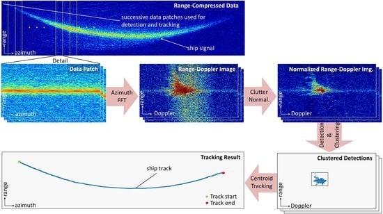
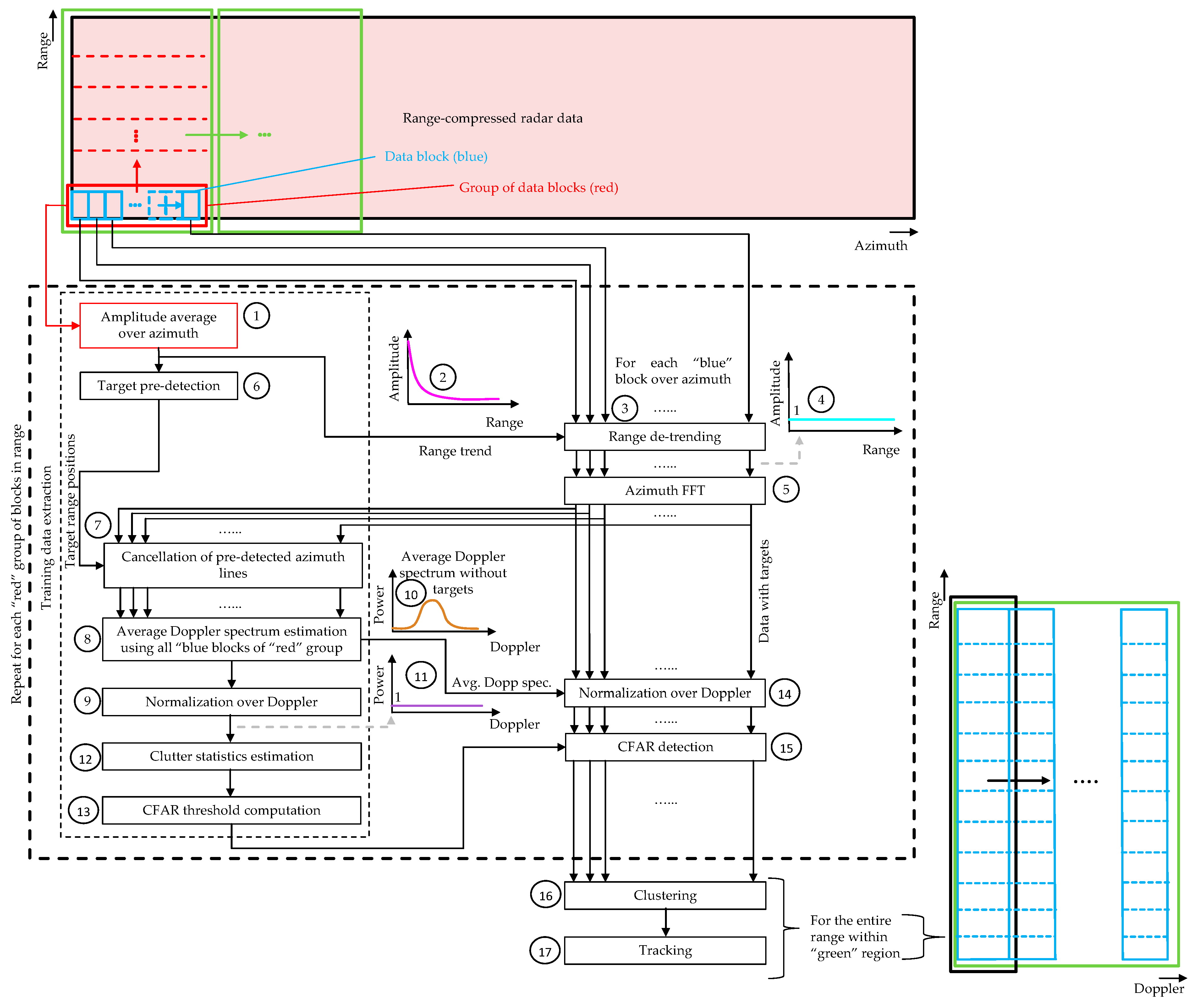
2. Principle of the Algorithm
- Extraction of a small data block from the RC radar data in time domain.
- Transformation of the data block to range-Doppler domain via azimuth fast Fourier transform (FFT).
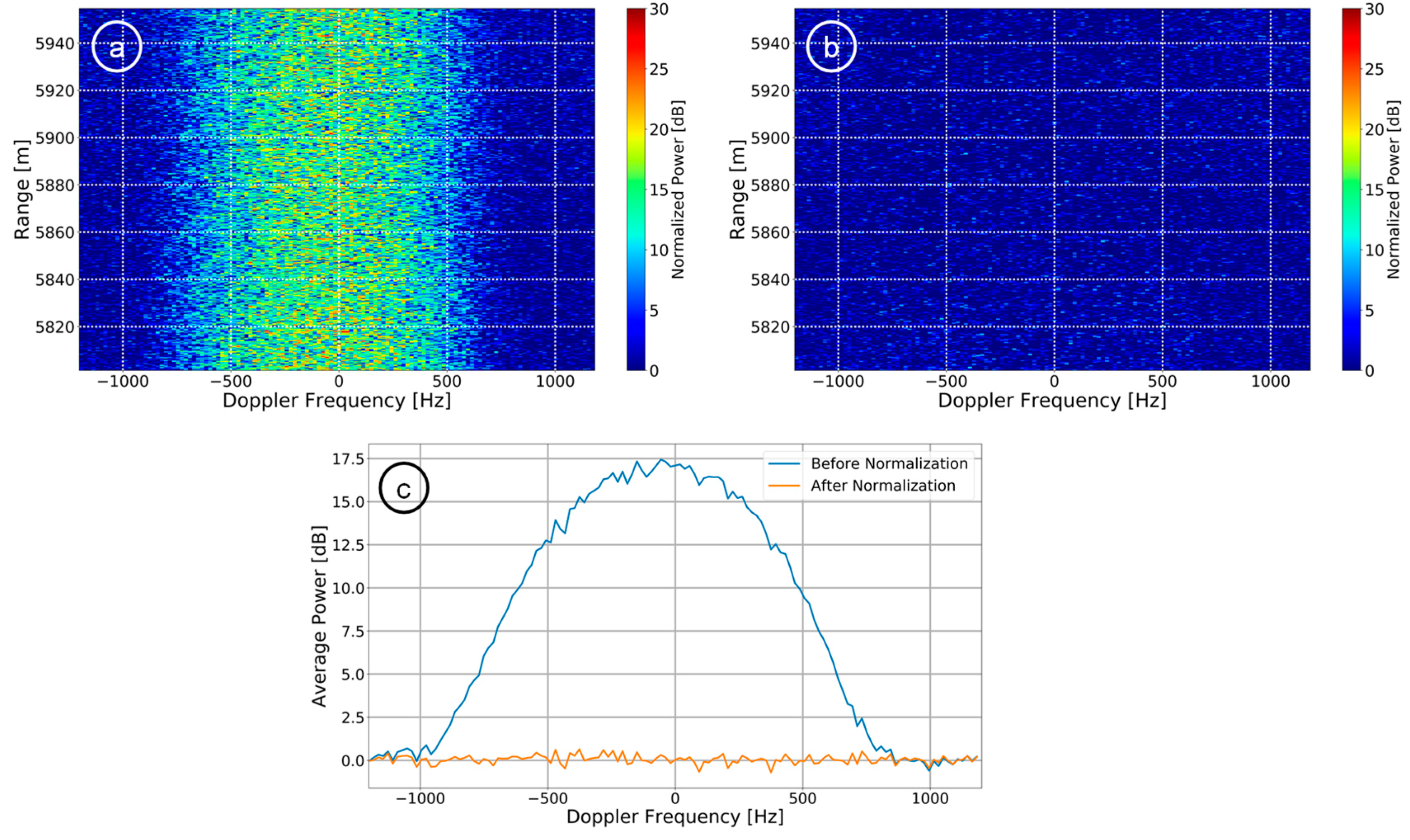
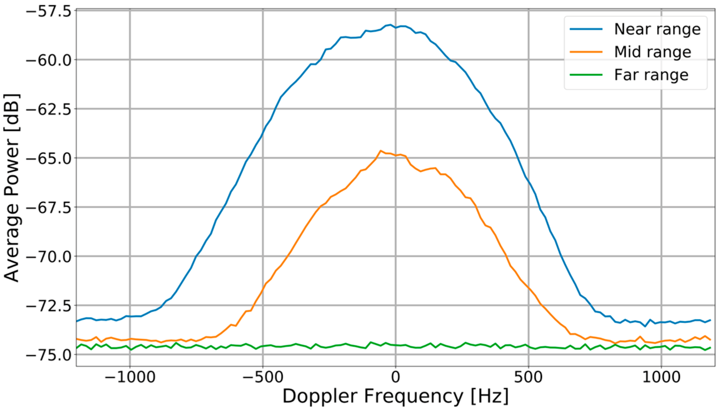
- Normalization over Doppler for achieving a “flat” spectrum.
- Estimation of the ocean clutter statistics.
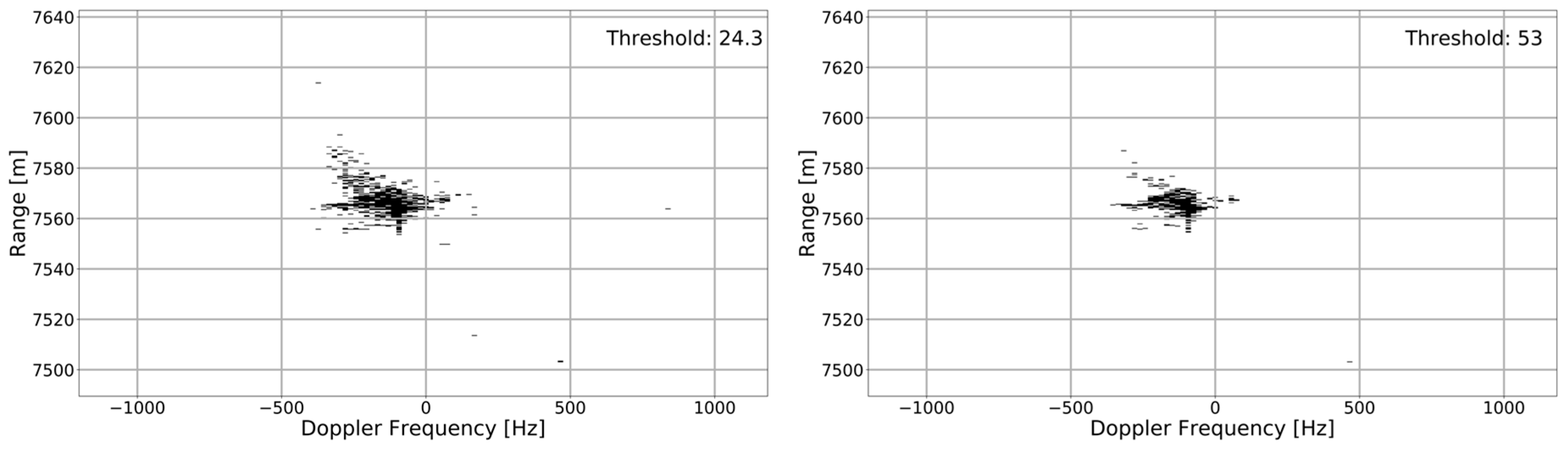
- Computation of a CFAR detection threshold based on the ocean clutter statistics.
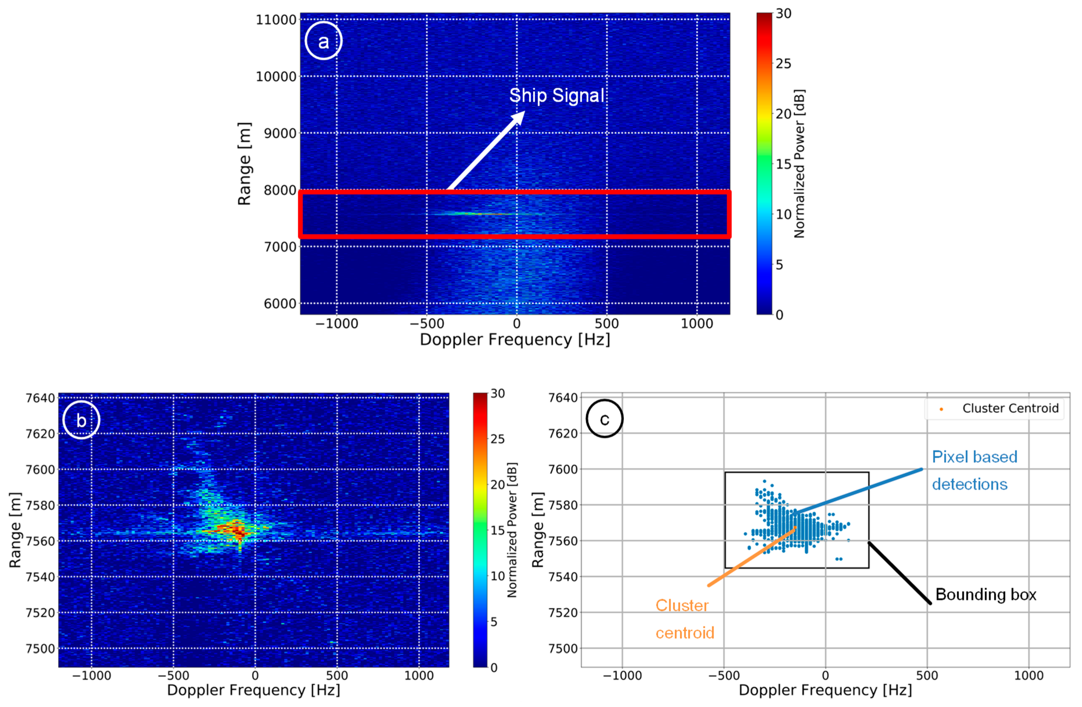
- Clustering of multiple detections to a single “physical object”.
- Tracking of the clusters, i.e., of the cluster centroid positions.
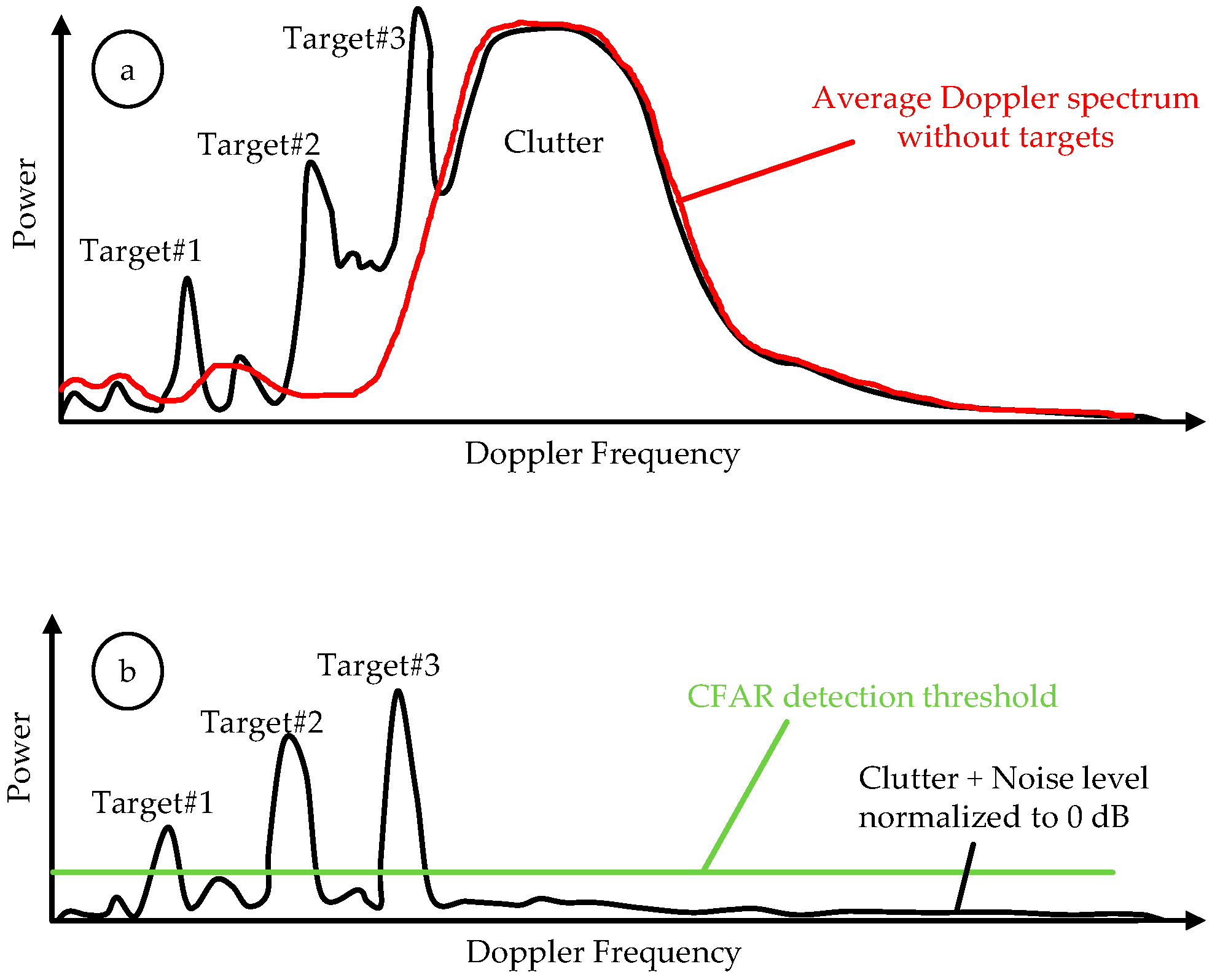
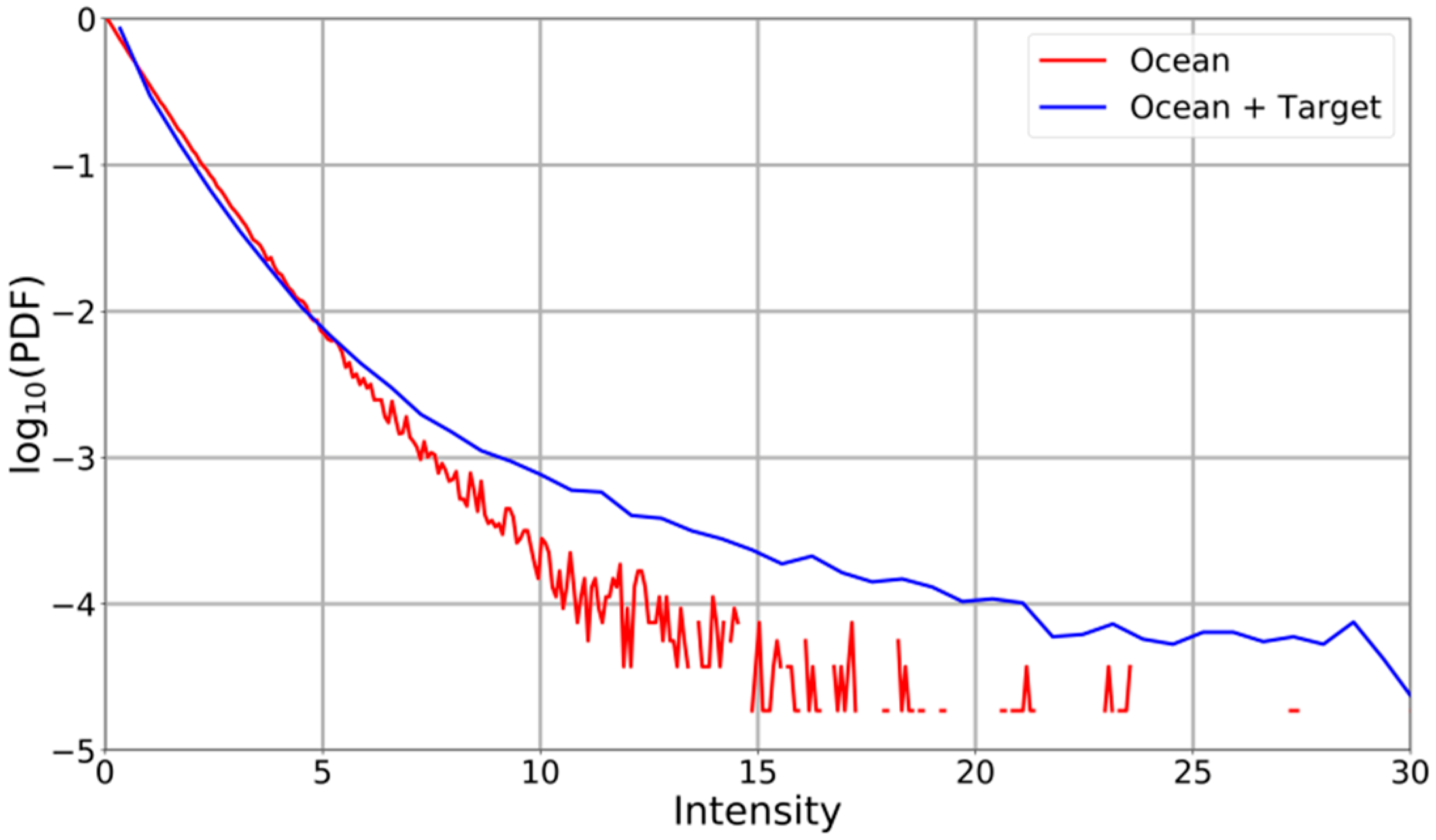
2.1. Importance of Clutter Normalization
2.2. Algorithm Block Diagram
3. Training Data Selection
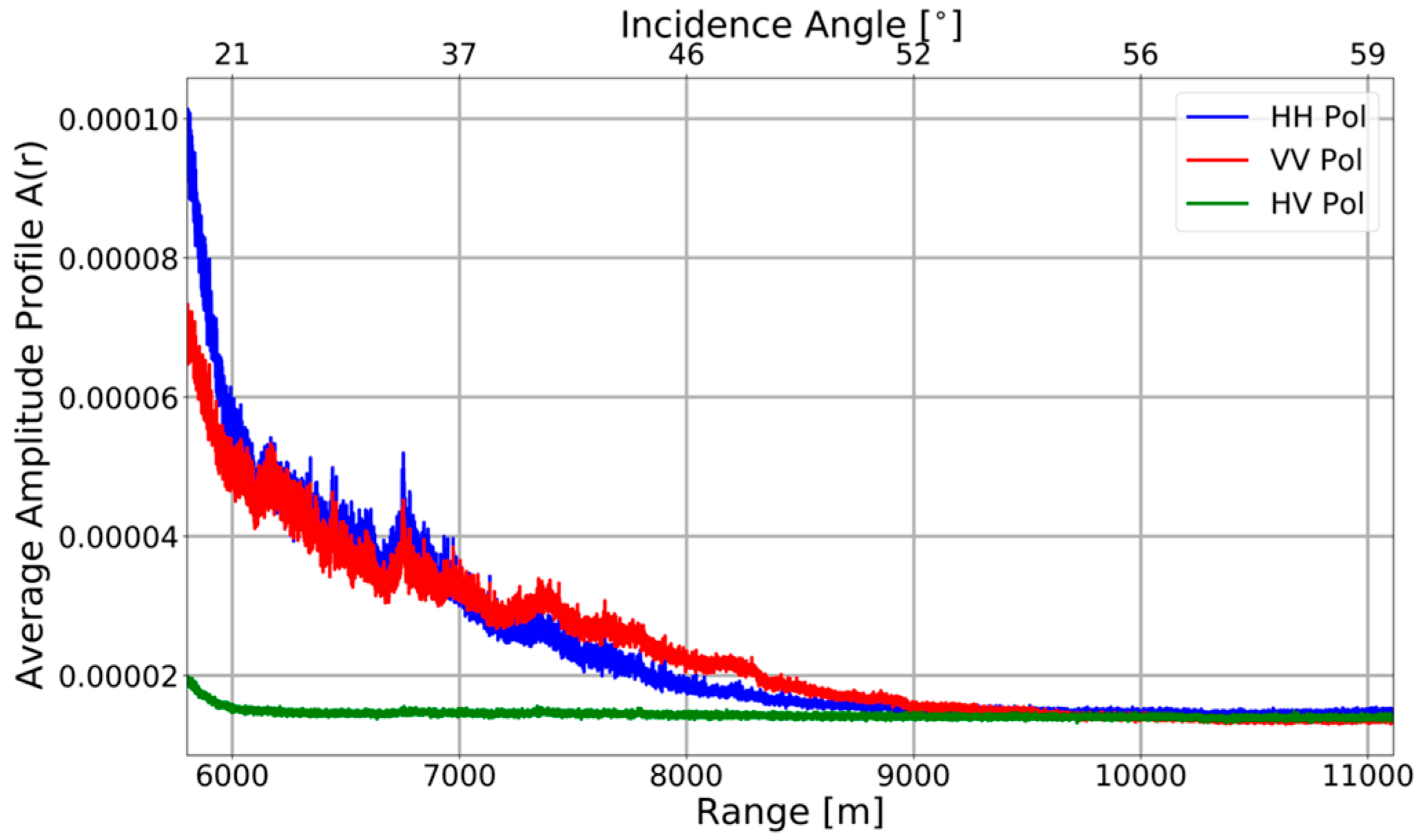
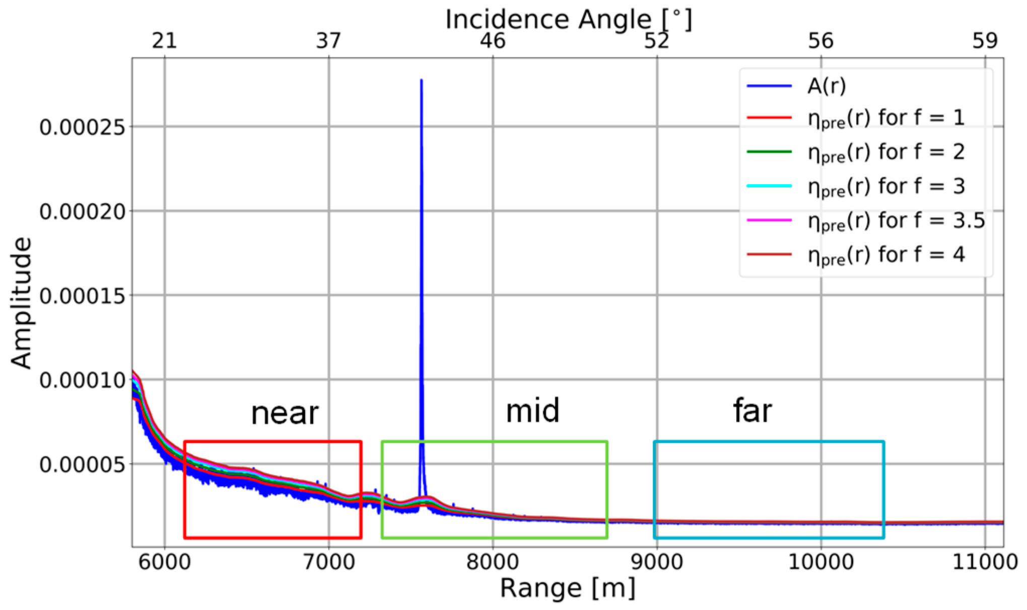
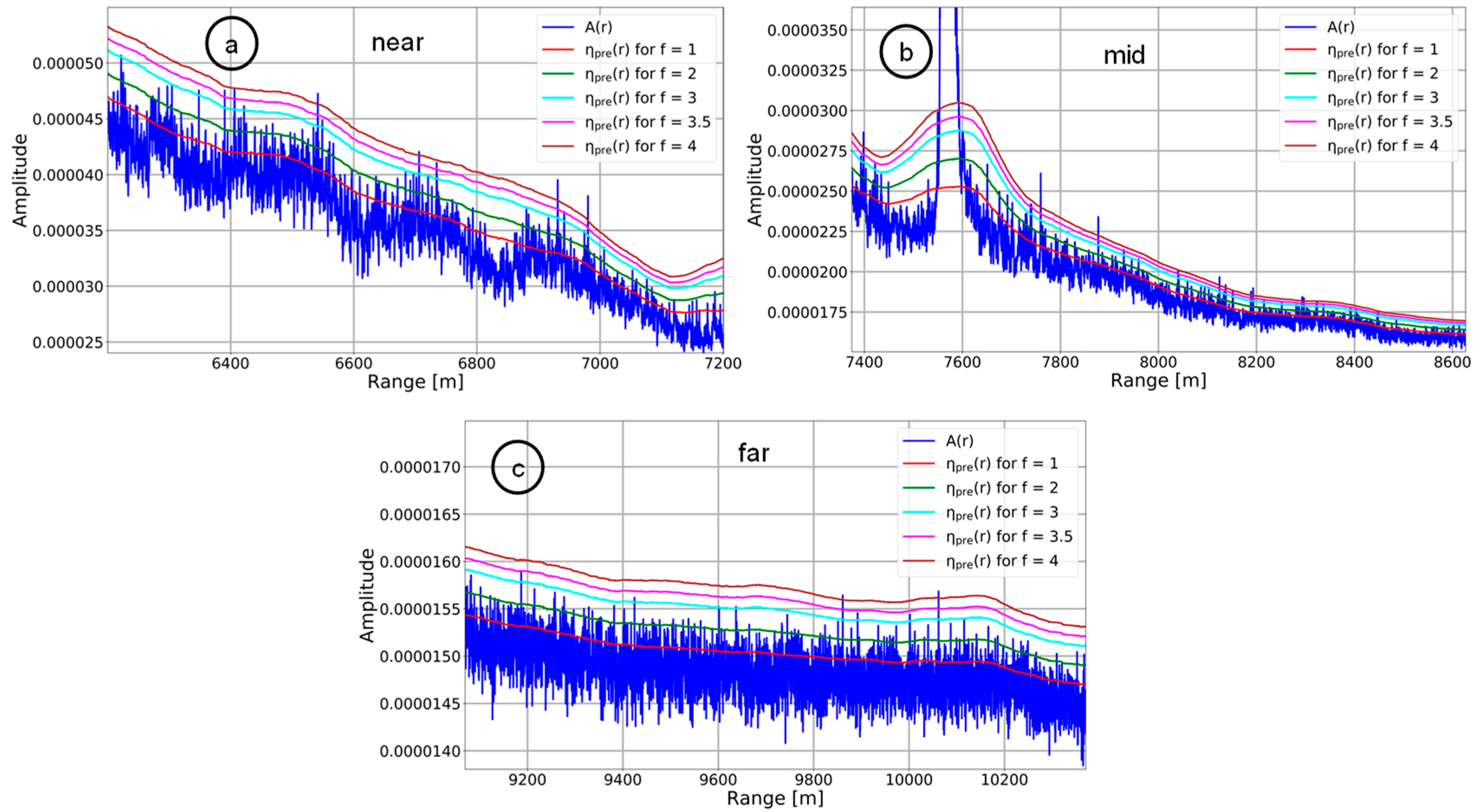
3.1. Target Pre-Detection
- RC radar data extraction in time domain (cf. green region in Figure 4).
- Incoherent summation over azimuth.
- Range-dependent adaptive threshold computation.
- Target peak detection and cancellation.
3.2. Clutter Normalization
3.3. Importance of Training Data Update
4. Clutter Statistics and Detection
4.1. K-Distribution
4.1.1. Method of Moments (MoM)
4.1.2. Non-Linear Least Squares Method (NLLSQ)
4.2. Chi Square Distribution
4.3. Tri-Modal Discrete (3MD) Texture Model
4.4. K-Rayleigh Distribution
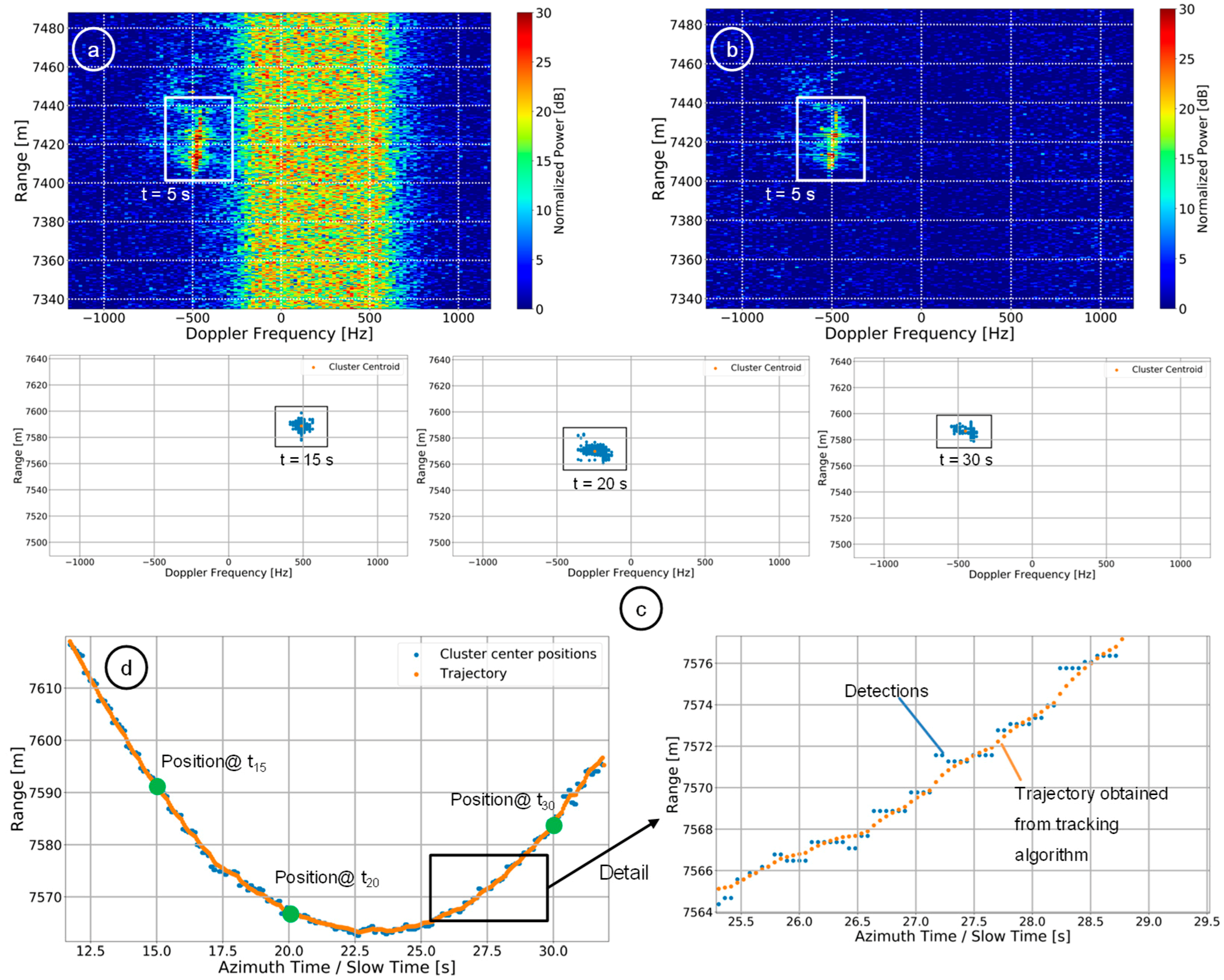
5. Clustering and Tracking
6. Experimental Results and Discussion
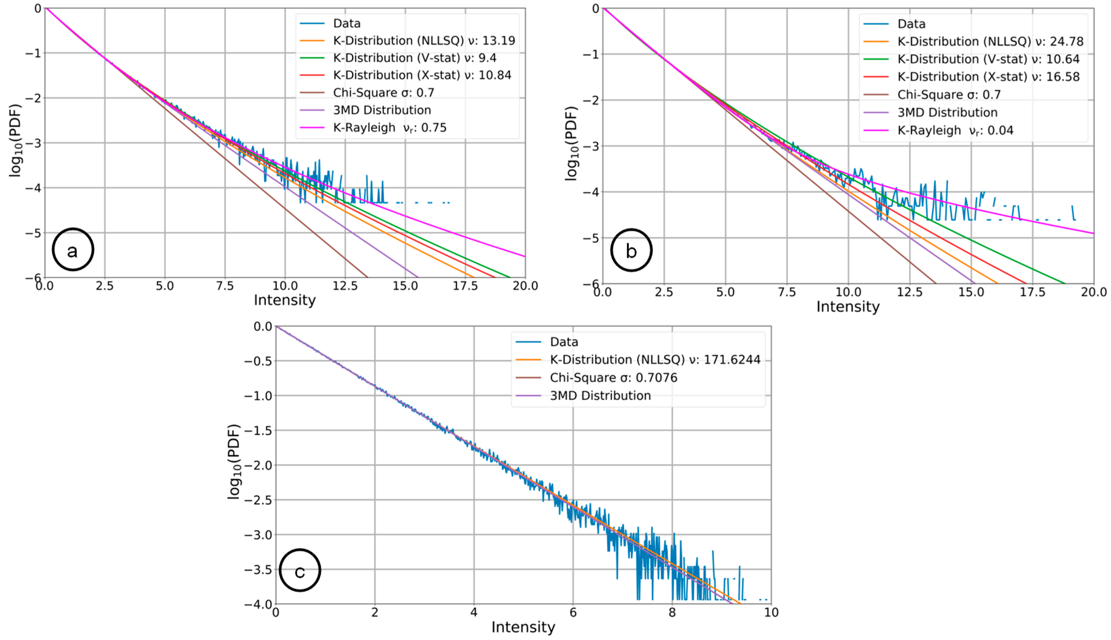
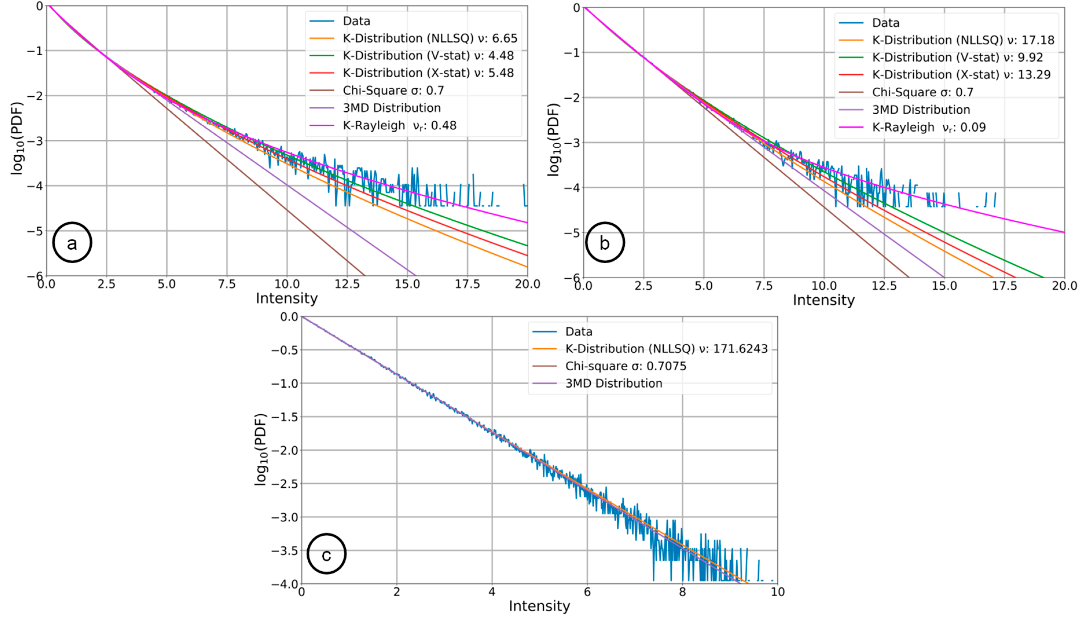
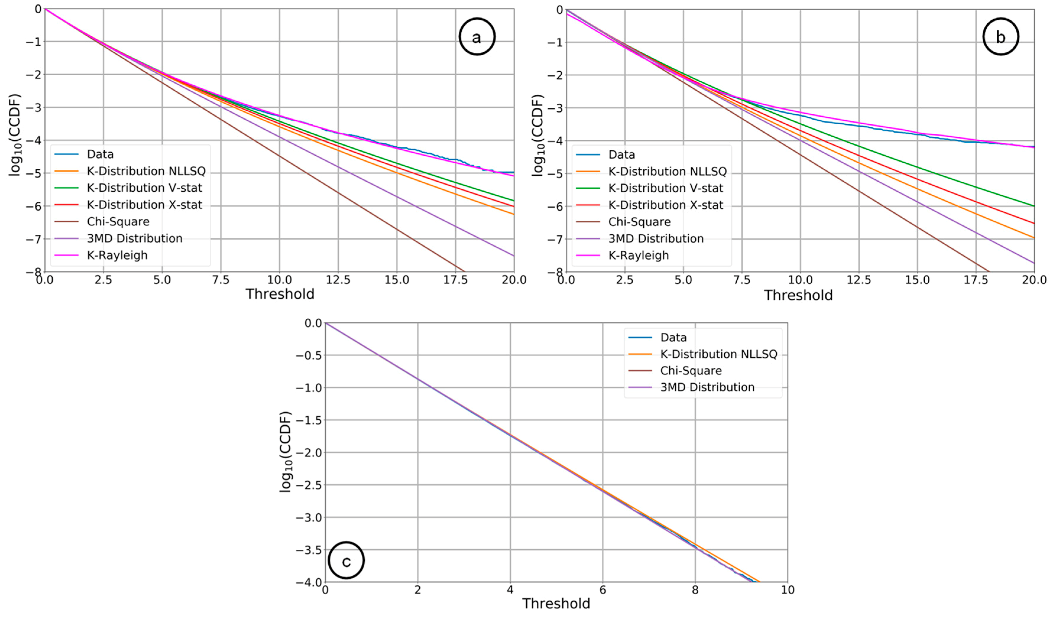
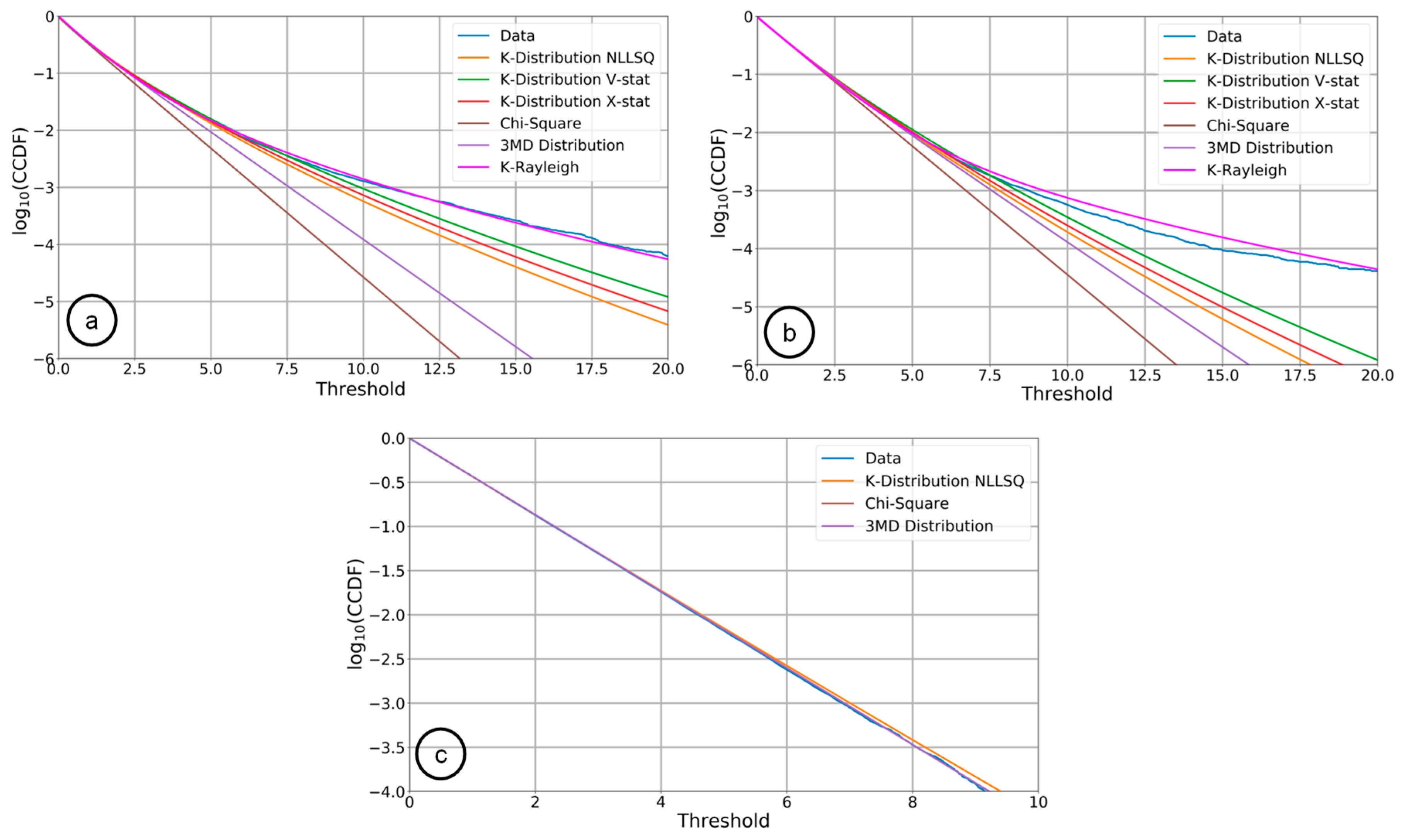
6.1. Clutter Model Fitting and Performance Evaluation
6.1.1. Threshold Error
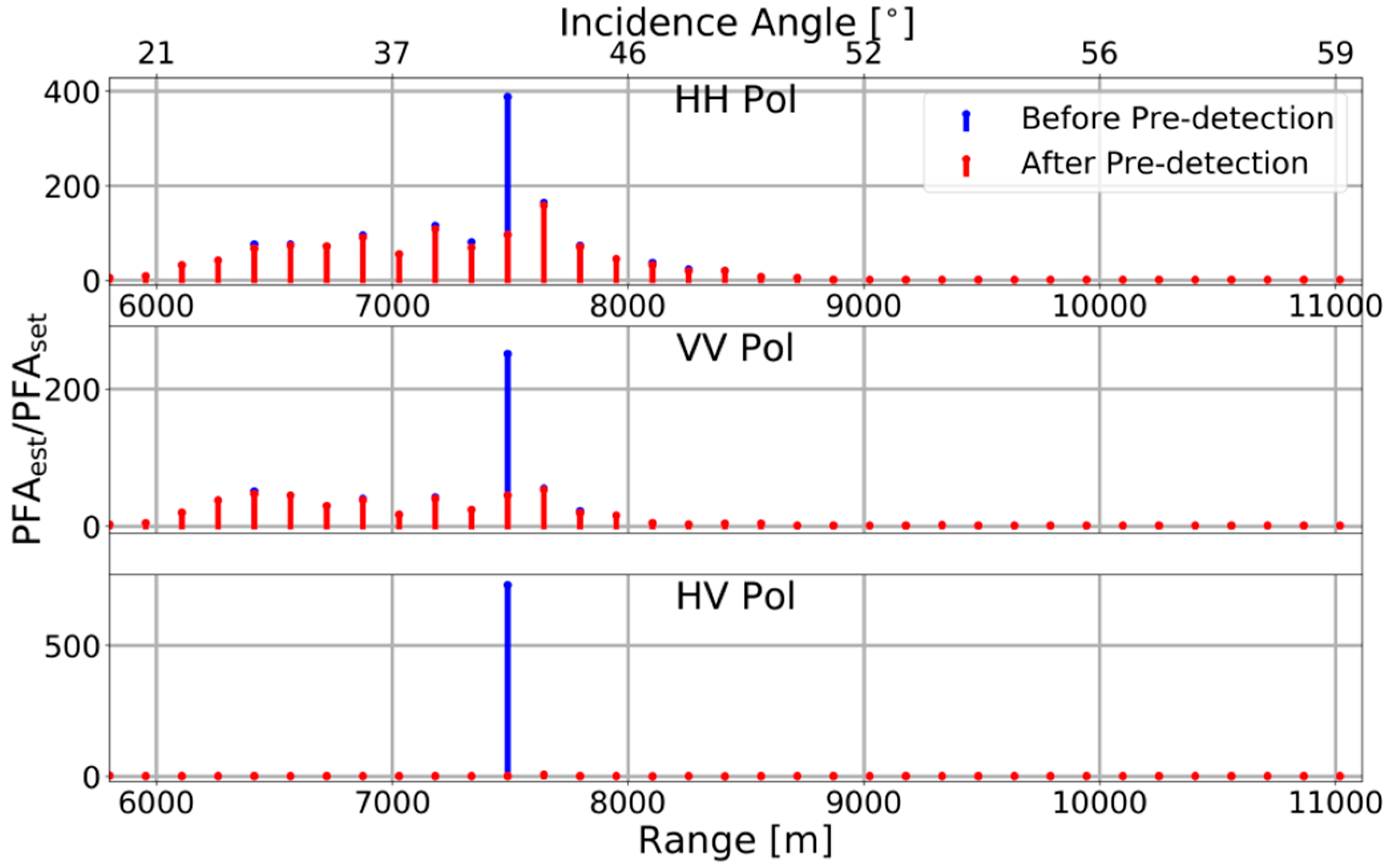
6.1.2. False Alarm Rate Error
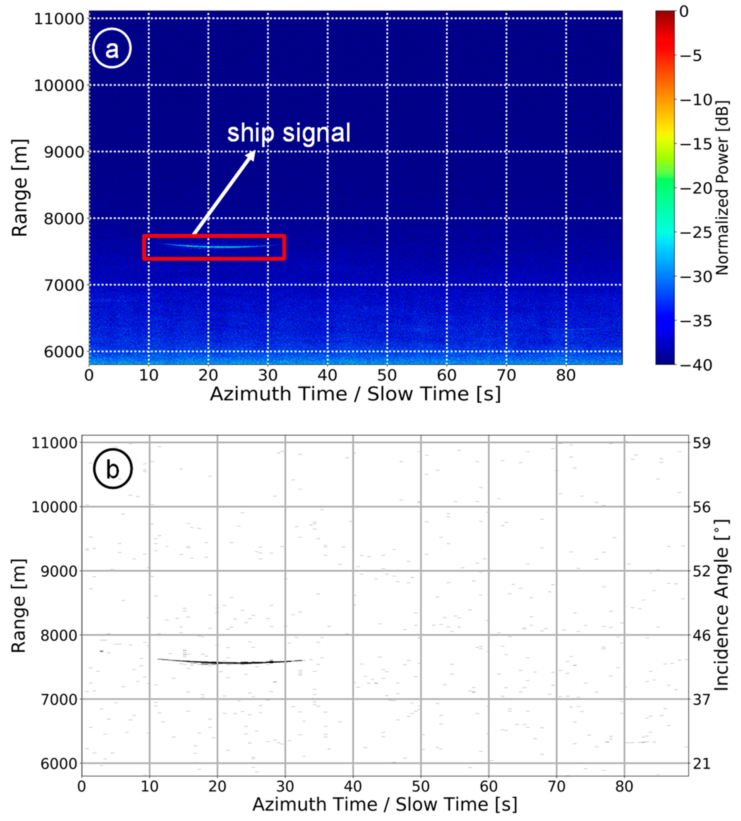
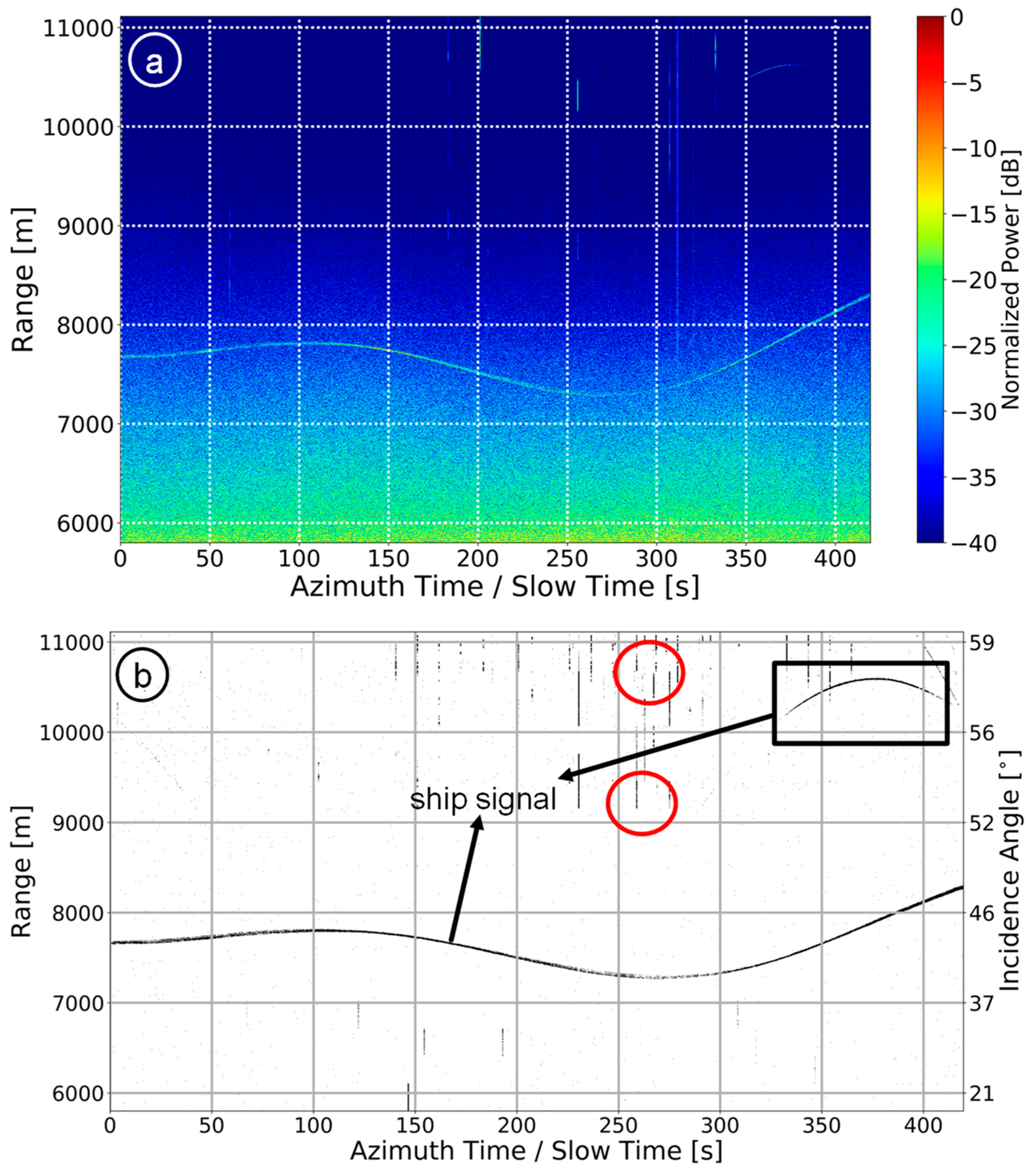
6.2. Detection Results
7. Conclusions
Author Contributions
Funding
Acknowledgments
Conflicts of Interest
References
- Te Hennepe, F.; Rinaldo, R.; Ginesi, A.; Tobehn, C.; Wieser, M.; Olsen, Ø.; Helleren, Ø.; Challamel, R.; Storesund, F. Space-based detection of AIS signals: Results of a feasibility study into an operational space-based AIS system. In Proceedings of the ASMS/SPSC 2010: 2010 5th Advanced Satellite Multimedia Systems Conference and the 11th Signal Processing for Space Communications Workshop, Cagliari, Italy, 13–15 September 2010; pp. 17–24. [Google Scholar]
- Eldhuset, K. An automatic ship and ship wake detection system for spaceborne SAR images in coastal regions. IEEE Trans. Geosci. Remote Sens. 1996, 34, 1010–1019. [Google Scholar] [CrossRef]
- Iervolino, P.; Guida, R.; Whittaker, P. A Model for the Backscattering from a Canonical Ship in SAR Imagery. IEEE J. Sel. Top. Appl. Earth Obs. Remote Sens. 2016, 9, 1163–1175. [Google Scholar] [CrossRef]
- Souyris, J.-C.; Henry, C.; Adragna, F. On the use of complex SAR image spectral analysis for target detection: Assessment of polarimetry. IEEE Trans. Geosci. Remote Sens. 2003, 41, 2725–2734. [Google Scholar] [CrossRef]
- Tings, B.; Velotto, D. Comparison of ship wake detectability on C-band and X-band SAR. Int. J. Remote Sens. 2018, 39, 4451–4468. [Google Scholar] [CrossRef]
- Biondi, F. A Polarimetric Extension of Low-Rank Plus Sparse Decomposition and Radon Transform for Ship Wake Detection in Synthetic Aperture Radar Images. IEEE Geosci. Remote Sens. Lett. 2019, 16, 75–79. [Google Scholar] [CrossRef]
- Biondi, F. Low-Rank Plus Sparse Decomposition, Multi-Chromatic Analysis and Generalized Likelihood Ratio Test for Ship Weak Detection, (L+S)-MCA-GLRT. In Proceedings of the 5th International Workshop on Compressed Sensing Applied to Radar, Multimodal Sensing, and Imaging (CoSeRa), Siegen, Germany, 10–13 September 2018; pp. 1–5. [Google Scholar]
- Brusch, S.; Lehner, S.; Fritz, T.; Soccorsi, M.; Soloviev, A.; van Schie, B. Ship surveillance with TerraSAR-X. IEEE Trans. Geosci. Remote Sens. 2011, 49, 1092–1103. [Google Scholar] [CrossRef]
- Baumgartner, S.V. Linear and Circular ISAR Imaging of Ships Using DLR’s Airborne Sensor F-SAR. In Proceedings of the International Conference on Radar Systems, IET Radar 2017, Belfast, UK, 23–26 October 2017. [Google Scholar]
- Martorella, M.; Pastina, D.; Berizzi, F.; Lombardo, P. Spaceborne radar imaging of maritime moving targets with the Cosmo-SkyMed SAR system. IEEE J. Sel. Top. Appl. Earth Obs. Remote Sens. 2014, 7, 2797–2810. [Google Scholar] [CrossRef]
- Liu, C.; Vachon, P.W.; Geling, G.W. Improved ship detection with airborne polarimetric SAR data. Can. J. Remote Sens. 2005, 31, 122–131. [Google Scholar] [CrossRef]
- Osman, H.; Blostein, S.D. Probabilistic winner-take-all segmentation of images with application to ship detection. IEEE Trans. Syst. Man Cybern. Part B Cybern. 2000, 30, 485–490. [Google Scholar] [CrossRef]
- Fingas, M.F.; Brown, C.E. Review of ship detection from airborne platforms. Can. J. Remote Sens. 2001, 27, 379–385. [Google Scholar] [CrossRef]
- Makhoul, E.; Baumgartner, S.V.; Jager, M.; Broquetas, A. Multichannel SAR-GMTI in Maritime Scenarios with F-SAR and TerraSAR-X Sensors. IEEE J. Sel. Top. Appl. Earth Obs. Remote Sens. 2015, 8, 5052–5067. [Google Scholar] [CrossRef]
- Cerutti-Maori, D.; Sikaneta, I.C.; Gierull, C.H. Ship Detection with Spaceborne Multi-channel SAR/GMTI Radars. In Proceedings of the 9th European Conference on Synthetic Aperture Radar, Nuremberg, Germany, 23–26 April 2012; pp. 400–403. [Google Scholar]
- Joshi, S.K.; Baumgartner, S.V. Sea clutter model comparison for ship detection using single channel airborne raw SAR data. In Proceedings of the EUSAR 2018: 12th European Conference on Synthetic Aperture Radar, Aachen, Germany, 4–7 June 2018; pp. 731–735. [Google Scholar]
- Melvin, W.L. A STAP overview. IEEE Aerosp. Electron. Syst. Mag. 2004, 19, 19–35. [Google Scholar] [CrossRef]
- Da Silva, A.B.C.; Baumgartner, S.V. Novel post-Doppler STAP with a priori knowledge information for traffic monitoring applications: Basic idea and first results. Adv. Radio Sci. 2017, 15, 77–82. [Google Scholar] [CrossRef][Green Version]
- Ward, J. Space-Time Adaptive Processing for Airborne Radar. IEE Colloq. Space Time Adapt. Process. 1998, 2/1–2/6. [Google Scholar]
- Reigber, A.; Scheiber, R.; Jager, M.; Prats-Iraola, P.; Hajnsek, I.; Jagdhuber, T.; Papathanassiou, K.P.; Nannini, M.; Aguilera, E.; Baumgartner, S.; et al. Very-high-resolution airborne synthetic aperture radar imaging: Signal processing and applications. Proc. IEEE 2013, 101, 759–783. [Google Scholar] [CrossRef]
- Watts, S.; Rosenberg, L. A comparison of coherent and non-coherent radar detection performance in radar sea clutter. In Proceedings of the International Conference on Radar Systems (Radar 2017), Belfast, UK, 23–26 October 2017; pp. 1–6. [Google Scholar]
- Rosenberg, L.; Watts, S. Model based coherent detection in medium grazing angle sea-clutter. In Proceedings of the 2016 IEEE Radar Conference, Philadelphia, PA, USA, 2–6 May 2016. [Google Scholar]
- Silva, A.B.C.; Baumgartner, S.V. Training Data Selection and Update for Airborne Post-Doppler Space-Time Adaptive Processing. In Proceedings of the EUSAR 2018: 12th European Conference on Synthetic Aperture Radar, Aachen, Germany, 4–7 June 2018; pp. 1285–1290. [Google Scholar]
- Baumgartner, S.V. Circular and Polarimetric ISAR Imaging of Ships Using Airborne SAR Sensors. In Proceedings of the EUSAR 2018: 12th European Conference on Synthetic Aperture Radar, Aachen, Germany, 4–7 June 2018; pp. 116–121. [Google Scholar]
- Cerutti-Maori, D.; Sikaneta, I.; Gierull, C.H. Optimum SAR/GMTI processing and its application to the radar satellite RADARSAT-2 for Traffic Monitoring. IEEE Trans. Geosci. Remote Sens. 2012, 50, 3868–3881. [Google Scholar] [CrossRef]
- Himonas, S.D.; Barkat, M. Automatic Censored CFAR Detection for Nonhomogeneous Environments. IEEE Trans. Aerosp. Electron. Syst. 1992, 28, 286–304. [Google Scholar] [CrossRef]
- Rohling, H. Radar CFAR Thresholding in Clutter and Multiple Target Situations. IEEE Trans. Aerosp. Electron. Syst. 1983, 19, 608–621. [Google Scholar] [CrossRef]
- El Mashade, M.B. Monopulse detection analysis of the trimmed mean level CFAR processor in nonhomogeneous situations. IEE Radar Sonar Navig. 1996, 143, 87–94. [Google Scholar] [CrossRef]
- Rickard, J.T.; Dillard, G.M. Adaptive Detection Algorithms for Multiple-Target Situations. IEEE Trans. Aerosp. Electron. Syst. 1977, 13, 338–343. [Google Scholar] [CrossRef]
- Cui, Y.; Zhou, G.; Yang, J.; Yamaguchi, Y. On the iterative censoring for target detection in SAR images. IEEE Geosci. Remote Sens. Lett. 2011, 8, 641–645. [Google Scholar] [CrossRef]
- Tao, D.; Anfinsen, S.N.; Brekke, C. Robust CFAR Detector Based on Truncated Statistics in Multiple-Target Situations. IEEE Trans. Geosci. Remote Sens. 2016, 54, 117–134. [Google Scholar] [CrossRef]
- Leys, C.; Ley, C.; Klein, O.; Bernard, P.; Licata, L. Detecting outliers: Do not use standard deviation around the mean, use absolute deviation around the median. J. Exp. Soc. Psychol. 2013, 49, 764–766. [Google Scholar] [CrossRef]
- Schafer, R.W. What is a savitzky-golay filter? IEEE Signal Process. Mag. 2011, 28, 111–117. [Google Scholar] [CrossRef]
- Bamler, R. Doppler frequency estimation and the Cramer-Rao bound. IEEE Trans. Geosci. Remote Sens. 1991, 29, 385–390. [Google Scholar] [CrossRef]
- Crisp, D.J.; Rosenberg, L.; Stacy, N.J.; Dong, Y. Modelling X-band sea clutter with the K-distribution: Shape parameter variation. In Proceedings of the 2009 International Radar Conference “Surveillance for a Safer World” (RADAR 2009), Bordeaux, France, 12–16 October 2009; pp. 1–6. [Google Scholar]
- Ward, K.D.; Tough, R.J.A.; Watts, S. Sea clutter: Scattering, the K distribution and radar performance. Waves Random Complex Media 2007, 17, 233–234. [Google Scholar] [CrossRef]
- Gierull, C.H. Numerical Recipes to Determine the Performance of Multi-Channel GMTI Radars; Defence R&D Canada: Ottawa, ON, Canada, 2011; p. 28.
- Jakeman, E. On the statistics of K-distributed noise. J. Phys. A Math. Gen. 1980, 13, 31–48. [Google Scholar] [CrossRef]
- Ward, K.D. Compound representation of high resolution sea clutter. Electron. Lett. 1981, 17, 561–563. [Google Scholar] [CrossRef]
- Greidanus, H. Applicability of the K distribution to RADARSAT maritime imagery. In Proceedings of the 2004 IEEE International Geoscience and Remote Sensing Symposium, Anchorage, AK, USA, 20–24 September 2004. [Google Scholar]
- Lombardo, P.; Oliver, C.J. Estimation of texture parameters in K-distributed clutter. IEE Proc. Radar Sonar Navig. 1994, 141, 196–204. [Google Scholar] [CrossRef]
- Blacknell, D.; Tough, R.J.A. Parameter estimation for the K-distribution based on [z log(z)]. IEE Proc. Radar Sonar Navig. 2001, 148, 309–312. [Google Scholar] [CrossRef]
- Moré, J.J. The Levenberg-Marquardt Algorithm: Implementation and Theory. In Numerical analysis; Springer: Berlin, Heidelberg, 1978; pp. 105–116. [Google Scholar]
- Abraham, D.A.; Lyons, A.P. Reliable methods for estimating the K-distribution shape parameter. IEEE J. Ocean. Eng. 2010, 35, 288–302. [Google Scholar] [CrossRef]
- Henschel, M.D.; Rey, M.T.; Campbell, J.W.M.; Petrovic, D. Comparison of probability statistics for automated ship detection in SAR imagery. Proc. SPIE 1998, 3491, 986–991. [Google Scholar]
- Gierull, C.H.; Sikaneta, I.C.; Defence, R.; Drdc, D.C. Improved SAR Vessel Detection Based on Discrete Texture. In Proceedings of the EUSAR 2016: 11th European Conference on Synthetic Aperture Radar, Hamburg, Germany, 6–9 June 2016; pp. 523–526. [Google Scholar]
- Gierull, C.H.; Sikaneta, I. A Compound-Plus-Noise Model for Improved Vessel Detection in Non-Gaussian SAR Imagery. IEEE Trans. Geosci. Remote Sens. 2018, 56, 1444–1453. [Google Scholar] [CrossRef]
- Rosenberg, L.; Watts, S.; Bocquet, S. Application of the K+Rayleigh distribution to high grazing angle sea-clutter. In Proceedings of the 2014 International Radar Conference, Radar 2014, Lille, France, 13–17 October 2014. [Google Scholar]
- Ester, M.; Kriegel, H.-P.; Sander, J.; Xu, X. A density-based algorithm for discovering clusters in large spatial databases with noise. In Proceedings of the International Conference on Knowledge Discovery and Information Retrieval, Portland, Oregon, 2–4 August 1996; pp. 226–231. [Google Scholar]
- Kalman, R.E. A New Approach to Linear Filtering and Prediction Problems. J. Basic Eng. 1960, 82, 35–45. [Google Scholar] [CrossRef]
- Tings, B.; Bentes, C.; Velotto, D.; Voinov, S. Modelling ship detectability depending on TerraSAR-X-derived metocean parameters. CEAS Space J. 2019, 11, 81–94. [Google Scholar] [CrossRef]


| Range-Doppler Image | Target SCNR [dB] |
|---|---|
| Before normalization (Figure 16a) | 24.02 |
| After normalization but without pre-detection (Figure 16c) | 14.20 |
| After normalization with pre-detection and target cancellation (Figure 16e) | 23.08 |
| Acquisition Parameters | Linear | Circular |
|---|---|---|
| Average platform velocity [m/s] | 91.4 | 83.55 |
| Platform altitude above ground [m] | 5638 | 5637 |
| Total observation time along azimuth [s] | 90 | 400 |
| Number of SAR image(s) used | 1 | 1 |
| Azimuth spacing [m] | 0.038 | 0.034 |
| Chirp bandwidth [MHz] for X- and L-band | 384, 150 | |
| Incidence angle range [°] | 15–60 | |
| Radar wavelength [m] for X- and L-band | 0.0306, 0.226 | |
| Pulse repetition frequency [Hz] | 2403.85 | |
| Total number of range samples | 17,723 | |
| Ground swath [km] | 8 | |
| Range Resolution [m] for X- and L-band | 0.39, 1.0 | |
| Range sample spacing [m] for X- and L-band | 0.3, 0.6 | |
| Azimuth antenna length [m] for X- and L-band | 0.3 m (Transmit), 0.2 m (Receive) (X-band) | |
| 0.3 m (Transmit), 0.3 m (Receive) (L-band) | ||
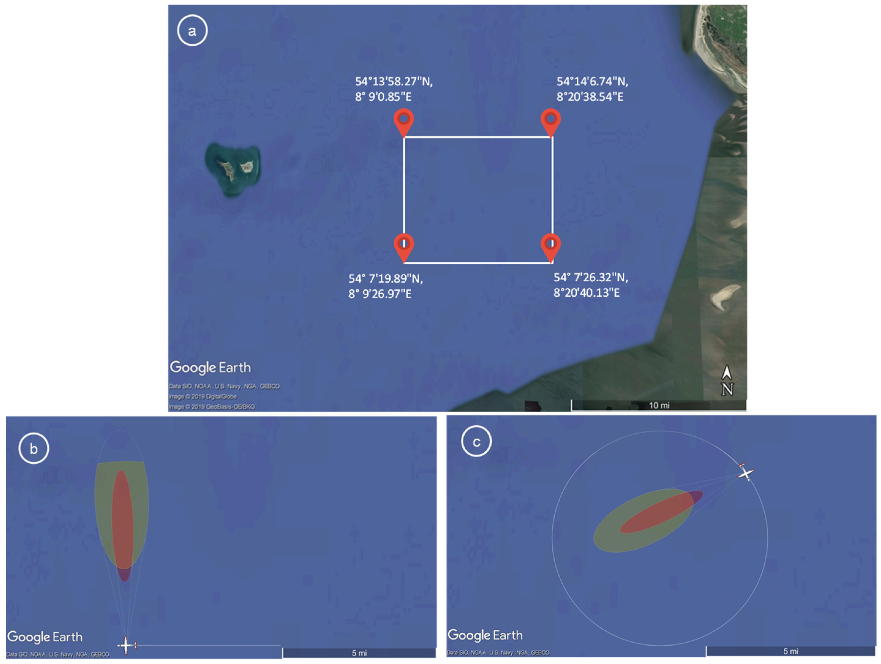
| Geographical coordinates | Shown in Figure 23a | |
| Clutter Models | Near Range | Mid-Range | Far Range | |
|---|---|---|---|---|
| CCDF | ||||
| K-NLLSQ | 3.97 | 8.01 | −10.34 | −2.16 |
| K-Vstat | 2.41 | 6.89 | - | |
| K-Xstat | 3.23 | 7.61 | - | |
| Chi-square | 6.98 | 8.87 | −10.34 | −4.98 |
| 3MD | 5.62 | 8.27 | −10.34 | −5.17 |
| K-Rayleigh | −5.79 | −0.26 | - | |
| Clutter Models | Near Range | Mid-Range | Far Range |
|---|---|---|---|
| CCDF | |||
| K-NLLSQ | 6.89 | 6.02 | −5.86 |
| K-Vstat | 5.19 | 4.60 | - |
| K-Xstat | 6.19 | 5.49 | - |
| Chi-square | 9.70 | 7.73 | −11.65 |
| 3MD | 8.94 | 6.94 | −10.86 |
| K-Rayleigh | −6.68 | 2.27 | - |
| Distribution Functions | Near Range | Mid-Range | Far Range |
|---|---|---|---|
| K-NLLSQ | 80.5 | 112.1 | 3.08 |
| K-Vstat | 35.1 | 57.1 | - |
| K-Xstat | 56.9 | 86.8 | - |
| Chi-square | 277.4 | 242.9 | 2.43 |
| 3MD | 149.2 | 135.9 | 1.56 |
| K-Rayleigh | 1.31 | 1.68 | - |
| Distribution Functions | Near Range | Mid-Range | Far Range |
|---|---|---|---|
| K-NLLSQ | 63.3 | 74.6 | 12.2 |
| K-Vstat | 30.6 | 38.9 | - |
| K-Xstat | 46.9 | 55.9 | - |
| Chi-square | 422.4 | 234.9 | 9.43 |
| 3MD | 257.9 | 154.7 | 7.73 |
| K-Rayleigh | 2.03 | 2.08 | - |
© 2019 by the authors. Licensee MDPI, Basel, Switzerland. This article is an open access article distributed under the terms and conditions of the Creative Commons Attribution (CC BY) license (http://creativecommons.org/licenses/by/4.0/).
Share and Cite
Joshi, S.K.; Baumgartner, S.V.; da Silva, A.B.C.; Krieger, G. Range-Doppler Based CFAR Ship Detection with Automatic Training Data Selection. Remote Sens. 2019, 11, 1270. https://doi.org/10.3390/rs11111270
Joshi SK, Baumgartner SV, da Silva ABC, Krieger G. Range-Doppler Based CFAR Ship Detection with Automatic Training Data Selection. Remote Sensing. 2019; 11(11):1270. https://doi.org/10.3390/rs11111270
Chicago/Turabian StyleJoshi, Sushil Kumar, Stefan V. Baumgartner, Andre B. C. da Silva, and Gerhard Krieger. 2019. "Range-Doppler Based CFAR Ship Detection with Automatic Training Data Selection" Remote Sensing 11, no. 11: 1270. https://doi.org/10.3390/rs11111270
APA StyleJoshi, S. K., Baumgartner, S. V., da Silva, A. B. C., & Krieger, G. (2019). Range-Doppler Based CFAR Ship Detection with Automatic Training Data Selection. Remote Sensing, 11(11), 1270. https://doi.org/10.3390/rs11111270