Improvement of Full Waveform Airborne Laser Bathymetry Data Processing based on Waves of Neighborhood Points

Abstract

Measurements of the topography of the sea floor are one of the main tasks of hydrographic organizations worldwide. The occurrence of any disaster in maritime traffic can contaminate the environment for many years. Therefore, increasing attention is being paid to the development of effective methods for the detection and monitoring of possible obstacles on the transport route. Bathymetric laser scanners record the full waveform reflected from the object (target). Its transformation allows to obtain information about the water surface, water column, seabed, and the objects on it. However, it is not possible to identify subsequent returns among all waves, leading to a loss of information about the situation under the water. On the basis of the studies conducted, it was concluded that the use of a secondary analysis of a full waveform of the airborne laser bathymetry allowed for the identification of objects on the seabed. It allowed us to detect further points in the point cloud, which are necessary in the identification of objects on the seabed. The results of the experiment showed that, among the area of experiment where objects on the seabed were located, the number of points increased between 150 and 550% and the altitude accuracy of the seabed elevation model even by 50% to the level of 0.30 m with reference to sonar data depending of types of objects.

1. Introduction

Measurements recording marine topography are among the basic tasks of hydrographic organizations worldwide. The development of maritime transport and the related increased ship traffic have led to emphasis being placed on the periodic monitoring of the seabed on the navigation pathways of ships in order to ensure safety. A maritime traffic disaster may lead to long-term pollution of the environment. Thus, increasing attention has been paid to the development of rapid methods of object detection and monitoring of possible obstacles found in a sea transport pathway. Thus far, sonar measurements have been used for this purpose [1], but also other remote sensing methods can be a data source for bathymetric measurements such as: stereophotogrammetry of underwater images [2] and image matching of photogrammetric images [3,4,5]. Nevertheless, special attention should be given to methods using airborne laser bathymetry, because this measurement method can be used as a supplement or a complete alternative to sonar data [6].

Airborne Laser Bathymetry (ALB) also called Airborne Lidar Hydrographic (ALH) is a technique which has become more and more important in recent years thanks to improved hardware and better processing software [7]. The first systems were introduced in the 1960s for military tasks to detect submarines. Based on these, it was proposed to use these systems for bathymetric measurements [8]. Today's bathymetric scanners are equipped with a green laser beam with a wavelength of 532 nm or a combination of a green and infrared beam with a wavelength of 1064 nm and measure the full waveform. Bathymetric lidar is also one of multispectral lidar systems [9]. The use of an additional infrared beam allows the derivation of some information about the water surface, because the beam is not able to penetrate the water column, but also does not guarantee that enough energy for its return [10]. A full waveform green beam should contain two peaks: (1) from the water surface (2) and from the bottom [11,12].

The objective of full waveform processing is to obtain the most precise information on the location and characteristics of the object (target) based on the received signal, the quality of which depends, among others, on the emitted beam, the reflecting object (target), and the receiver. Full waveform processing algorithms can be divided into three groups [11,13] as follows:

• Return detection (echo): this method focuses on the location of the target with the omission of radiometric traits. The echo locations are detected directly by using the threshold, centre of gravity, and the maximum or zero crossing of the second derivatives [14].
• Mathematical approximation: this method is based on fitting a mathematical function into the recorded waveform. Examples of such functions include Gaussian decomposition, Weibull function, generalized Gaussian function, and more. Chauve et al. [15] proposed the mixture of Lognormal and generalized Gaussian functions to waveform decomposition. Abdallah et al. [16] used a triangular function for full waveform processing. Adaby et al. [17] and Ding et al. [18] presented the combination of a quadrilateral function with Gaussian function. They used three functions: two Gaussian functions for the water surface and the water bottom contribution and a quadrilateral function to fit the water column. Wang et al. [19] proposed the multiscale wavelet analysis for waveform characterization and average tree height estimation.
• Deconvolution: this method consists of removing components of the emitted wave from the received signal. Examples of this method include Wiener filter deconvolution [20], Richardson–Lucy deconvolution [21], expectation maximization (EM) deconvolution [22], exponential decomposition with implicit deconvolution [23], and wavelet deconvolution [24].

The scope of research problems solved thus far indicates cognitive gaps in the use of all data obtained from airborne laser bathymetry for seabed monitoring. Attempts have been made to determine the optimum conditions for obtaining data from ALB [7] and their processing [11,18], yet, a need exists for further research on the analysis of full waveform airborne laser bathymetry and development of the obtained data. Numerous factors such as visibility in water or vegetation have a negative impact on the received signal [25], which results in difficulties in the identification of the second and subsequent returns during full waveform processing. Parrish el al. [22] and Pan et al. [26] suggest that there is no superior full waveform processing algorithm for all bathymetric situations. Because of the facts listed above, a secondary analysis of received signal waves in which only one return was identified, including the neighbouring correctly identified points, was the motivation for the present study. The aim of this paper was to investigate further lidar return waveform in waves with recognized one echo to detect the following echoes. To achieve the goal, a reprocessing of the full waveform from airborne laser bathymetry data was used based on a Gaussian decomposition function and neighbourhood waves with two or more echoes in the point cloud. The novelty of this method is using neighbouring waves with two or more returns to approximate the location of second echo in waves with one return by using the search window.

After the introduction, in the second section, the collected data, test area, and methodology, including Gaussian decomposition function, are described. The third section presents the results of methodology on the selected examples with a validation of the results in comparison to point clouds without an improvement and with reference sonar data. The obtained results are discussed and used to draw conclusions in the final part of the paper.

2. Materials and Methods

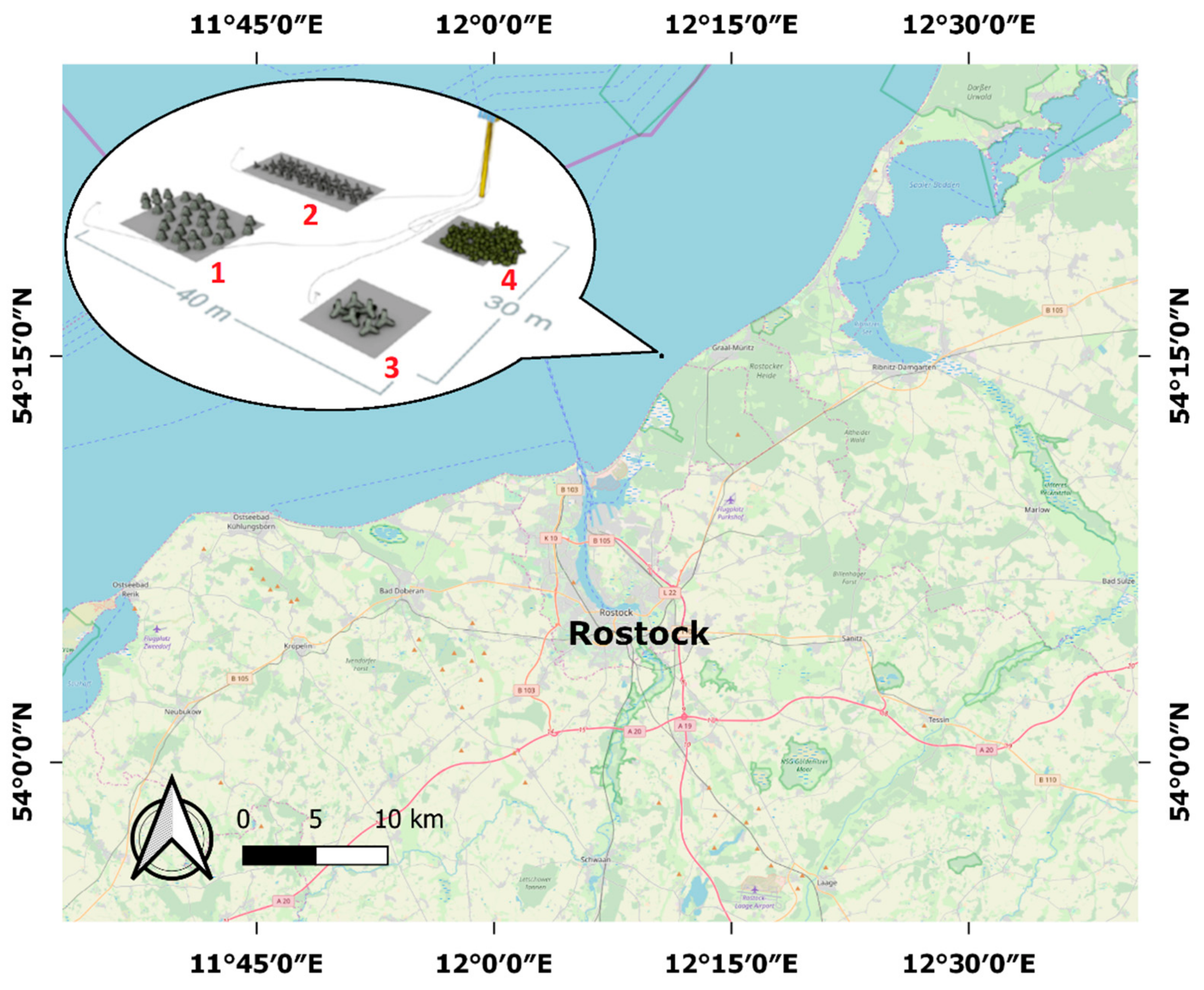
2.1. Test Object

The test object is the Rosenort artificial reef located in the Baltic Sea approximately 25 km north of Rostock (Figure 1) with the adjacent area of 5320 m². It was created as part of a research project, with one of its objectives being the study of the population and behavior of cod in the Baltic Sea. The Rosenort reef was created in 2009, and it comprises four artificially created fields, which are made of the following:

• 30 cut concrete cones,
• 50 two-ton concrete tetrapods,
• 6 six-ton concrete tetrapods,
• 180 tons of stone.

The objects are located approximately 2 km from the shoreline at the mean depth of approximately 6 m. It is an area of ichthyological reserve, where fisheries, angling, and anchoring are prohibited.

Data from airborne laser bathymetry used in the experimental portion of the present publication were obtained within the framework of the project entitled “Investigation on the use of airborne laser bathymetry in hydrographic surveying” implemented by the German Maritime Shipping Agency in Rostock (BSH Rostock) and the Institute for Photogrammetry and GeoInformation of the Leibniz University in Hannover. The data were obtained in August 2013 by using the AHAB Chiroptera scanner with the flight altitude of 400 m, the horizontal accuracy of which is 0.75 m for green beam and 0.2 m for red beam, and the accuracy of depth rating is 0.15 m (interpreted as the accuracy of altitude measurement). The laser scanner uses an infrared laser at 1064 nm with peak measurement frequency 400 kHz for water surface detection and green laser with a wavelength of 532 nm at 36 kHz for sea bottom measurement [27]. The system scans ground in a predefined pattern of an elliptical shape. The angle between the scan direction and the nadir is 20°. The sensor reaches in shallow water about one Secchi depth. Under Secchi depth should be understood as the maximal depth at which the human eye can detect a white or white-black disk in the water [28].

Within the study area, 3 points/m² were recorded on an average. During the measurement, 14,902 full waveforms were recorded. The total of 30,379 points have been measured, with the greatest depth for a single point of 6.7 m at the sea bottom. The minimum water depth over the obstacles was 4.5 m and around the objects 6.1 m. In the experiment, 575 waves were analyzed that were touching the object located on the seabed. 215 waves provided a first and a second echo, and 360 waves provide only one return. The area of the four analyzed objects is about 410 m². The preliminary density on the objects was very low (0.4 point per m²). The first extraction of the discrete form of the LiDAR data (point cloud) from full waveform was processed with the sensor dedicated AHAB LSS software. The software used three different thresholds to analyze the data [29]. One threshold is a linear decaying slope use for threshold peaks from the backscatter curve. The slope starts at the sample position corresponding to the water surface. Two thresholds are used to set a minimum allowed peak amplitude. The parameters have been automatically selected in the best way for all waves. For the most part, it provided points from the second echo, however, for some beams, this was not exactly the most correct solution. This resulted in the lack of a second return corresponding to the sea bottom points. Secondary analysis using Gaussian decomposition helped to find points from these waves and this was the aim of presented methodology.

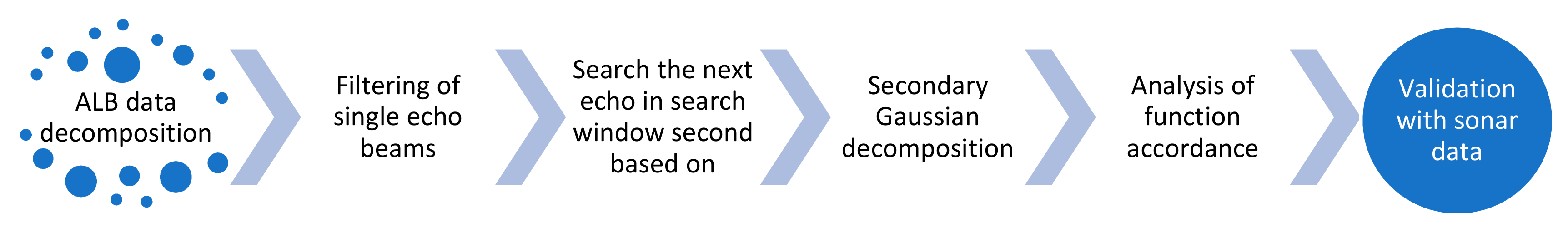
2.2. Methodology

The Gaussian decomposition function, which has been used in the analyses of the present study, belongs to the group of mathematical approximation, and it is widely used in the process of full waveform analysis from airborne lidar topography and bathymetry [11]. The Gaussian function fitting gives overall good results for all kinds of areas [15]. For a single return, this function assumes the following form:

$$f\left(t\right)=\alpha e^{\frac{-{\left(t-\mu \right)}^2}{2{\sigma }^2}}$$

(1)

where:

• α—wave amplitude,
• μ—position,
• σ—standard deviation,
• t—time/sample.

In the classic probability density function of a normal distribution, μ is determined as a mean, whereas in the literature, μ is mentioned as the position of Gaussian [11,12]. However, more than one return is recorded in the airborne laser bathymetry. According to the theoretical assumptions, at least two echoes should occur, one from the water surface, and the second from the bottom [16,30]. In addition, the number of returns may be determined iteratively [31,32], and in such a case, the Gaussian decomposition function assumes the following form:

$$f\left(t\right)={\displaystyle \sum }_{i=1}^N{\alpha }_i{e}^{\frac{-{\left(t-{\mu }_i\right)}^2}{2{\sigma }_i^2}}$$

(2)

where:

• N—number of Gaussian components,
• α_i—amplitude of i-th component,
• μ_i—position of i-th component,
• σ_i—standard deviation of i-th component.

To determine the parameters of Gaussian function, the minima of target function $f_c$ are found, which is defined as follows:

$$f_c=\frac{1}{N}\parallel W_R\left(t\right)-{\displaystyle \sum }_{i=1}^N{\alpha }_i{e}^{\frac{-{\left(t-{\mu }_i\right)}^2}{2{\sigma }_i^2}}\parallel$$

(3)

where:

• W_R(t)—received wave,
• N—number of Gaussian components,
• α_i—amplitude of i-th component,
• μ_i—position of i-th component,
• σ_i—standard deviation of i-th component.

$$\parallel x\parallel ={\displaystyle \sum }_{i=1}^n{\left(x_i\right)}^2$$

(4)

The workflow of secondary ALB data processing was present in Figure 2.

The first step in data processing was the decomposition of a full wave form in AHAB LSS software dedicated for ALB data. After observing problems with a large number of missing points of objects located on the seabed, a decision was made to search for beams with one peak. The preliminary location of a second echo in the full waveform of neighbouring beams was known from neighbouring waves, which was selected by nearest neighbour algorithm. Based on this, it was assumed that the next echo in wave with one return should be located close to the same sample. Using the search window, 30 samples were taken before and after the approximated location. For such a selected part of beams in the Matlab software, an attempt was made to fit the Gaussian function. The new points have been added to the point cloud if parameters of Gaussian function were calculated in in accordance with the function. To obtain the final echo parameters, the non-linear least-square method using the Levenberg–Marquardt algorithm [33,34] was used. Waveform fitting with the Levenberg–Marquardt technique was used and described by many authors [12,15,31,35,36]. Based on Reference [31], the criterion of Gaussian fitting was that the standard deviation of the residual difference must be less than three times the standard deviation of the background noise within the observed waveform. The final step of workflow was the validation of the data. In this case, the data were compared to the preliminary results and validated with multibeam sonar data that represented the digital surface model of the seabed in a resolution of 1 m.

For the process of the secondary analysis of full reflected waveform from airborne laser bathymetry, beams were selected in which only one peak was recorded in the first processing. In the analyzed test data, this condition was met by 575 points demonstrated by the blue color in Figure 3A, in which only the echo from the water surface was identified. The gaps in ALB point clouds can be observed in areas that are the most important due to occurrence of the objects located on the sea bottom (Figure 3B).

3. Results

In this section, the effect of method application on single waves was presented. In this part, positive (detection) and negative (lack of detection) effects of using Gaussian decomposition were also illustrated. The obtained results were compared with those received in preliminary analysis without using secondary processing with Gaussian function and validated with sonar data as reference value showing the truth surface of sea bottom.

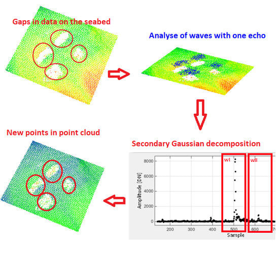
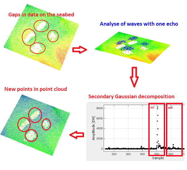
3.1. Secondary Analysis of Airborne Laser Bathymetry (ALB) Full Waveform

To verify the correctness of the concept of selecting waves with one detected echo for further analyses, randomly selected neighboring waves from the area were verified. Eight subsequent waves are presented in Figure 4. The first four waves (pink) are those in which two echoes were registered, whereas the four successive waves have only one echo registered. For all waves, a clear echo is present near the 500-sample from the water surface and approximately 630 sample in four first waves. On the basis of these observations, waves with one echo recorded were subjected to a secondary analysis.

The subsequent process of secondary analysis of full waveform from airborne laser bathymetry is presented in an example of one random wave. An echo from the water surface can be seen in Figure 5 at the 500-sample (wI). In the area of the 630-sample, a minor amplitude jump (peak) can be seen relative to the neighbouring samples (wII fragment) omitted in the first wave analysis process, during which the entire wave was analysed. A similar amplitude jump can be observed in the 400-sample; however, because this is a reading before the wI fragment, it was ignored (elements above water surface).

The approximate location of second peak in wave with one echo was determined by using the location (μ) of second peak in the neighbouring wave with two echoes. Subsequently, a window was used that collected 30 closest samples from one wave in both directions. Several window sizes have been tested, but the higher window in this case did not alter the results. The algorithm is adapted to change the size of the window in the case of other water depths. 30 samples of the wave in the water correspond to approximately 1.4 m, which exceeds the size of artificially created objects. In such window, a method of fitting Gaussian decomposition function was applied, the maximum of which defined the location of new points. The application of the window solves the problem of the number of returns, because, in this approach, there should be only one Gaussian. Fitting of such function with the non-linear least-square method using the Levenberg–Marquardt algorithm is presented in Figure 6, for which example coefficients were determined as follows: α = 872.4, μ = 616.6, σ = 1.766.

Having analyzed all waveforms with a single echo and applying filtration, 215 new points were detected, which were added to the point cloud. Newly detected points filled the gaps in the sites of the artificial reef. In the remaining analyzed waves, the noise was too high (Figure 7A) or too little energy was recorded (Figure 7B) to enable fitting the Gaussian decomposition function in the presented approach. These waves require further analyses and in this approach the waves remained with one echo on the water surface.

3.2. Validation of New Points

The newly detected points in the cloud were validated in comparison to point clouds generated in preliminary processing of full wave form data. The visual effect of this comparison can be seen in Figure 8. It is visible that the firstly detected points show the objects omitted in preliminarily processed point clouds (Figure 8D) that caused negative values for objects on the sea bottom reaching below −1 m difference (Figure 8A). A hillshade model of reference data overlaid with height difference presents the improvement of the results (Figure 8B), but some noise for plain area reaching 0.25 m is visible for both models. The minimum value of height difference for the second model was only −0.58 m. Some maximum values appeared instead on the level of 1 m. Generally speaking, in Figure 8C the difference between the preliminary and the secondary analysis showed how new points helped in more proper modelling of objects on sea bed. This is also visible in Figure 8D–F where the same scale was used in the 3D visualization. Improvement results (Figure 8E are much more similar to the reference data (Figure 8F) than preliminary ones (Figure 8D). Besides new maximum values, the improvement is also related to the detection of new points being the minimum between the already detected maximus. New detected points provide new detailed information about the object.

Received data were also evaluated with independent multibeam sonar in the form of a raster with pixel size of 1 m. Figure 9 presents discrepancies between the altitudes obtained from the sonar and lidar bathymetry in the form of a histogram. The point distribution of new points (approximately 70%) can be observed within the range of ±0.5 m. The mean height difference for all measured points on the seabed with new points is −0.02 m, and standard deviation of 0.11 m. Before finding new points, it was respectively −0.04 m for mean height difference and 0.16 m for standard deviation. Because of the considerable diversity of topography at the site of piled concrete blocks and the size of reference data pixel, the obtained results were divided for 4 test objects on the sea bottom without influence of plain seabed fragments. The results in

Table 1. Comparison of point clouds statistics and accuracy of seabed elevation model in the area of objects on the sea bottom. Calculations were made with respect to sonar data for the results of secondary analysis of full waveform on the objects.

	Airborne Laser Bathymetry (ALB) Data Processing/Object Number	1 (30 Cut Concrete Cones)	2 (50 Two-Ton Concrete Tetrapods)	3 (6 Six-Ton Concrete Tetrapods)	4 (180 Tons of Stone)
Number of points in point clouds	preliminary processing	19	28	12	41
	secondary analysis	97	40	77	101
	Change [%]	411	43	542	146
Density of point cloud on the objects [pts/m2]	preliminary processing	0.18	0.4	0.13	0.30
	secondary analysis	0.91	0.57	0.82	0.74
	Change [%]	406	43	531	147
Mean value of vertical error for surface model of objects [m]	preliminary processing	−0.19	−0.39	−0.11	−0.41
	secondary analysis	−0.11	−0.12	−0.10	−0.07
	Difference	0.08	0.27	0.01	0.34
Standard deviation of vertical error for surface model of objects [m]	preliminary processing	0.19	0.37	0.15	0.45
	secondary analysis	0.24	0.32	0.21	0.28
	Difference	0.05	−0.05	0.06	−0.17
Root Mean Square Error (RMSE) for surface model of objects [m]	preliminary processing	0.27	0.54	0.18	0.61
	secondary analysis	0.26	0.34	0.23	0.29
	Difference	−0.01	−0.20	0.05	−0.32

provide statistics calculated for point clouds and for surface interpolated from observations.

In Table 1, statistics for improved point clouds on the objects were shown in relation to the preliminarily obtained data without improving and with reference to sonar data. The results show that statistics for point clouds improved significantly. Depending on the type of objects (cones, smaller and bigger tetrapods, and stones), there was an increase in the number of points for 4 types from 43 to 542% depending on type of the object. As a consequence of these improvements, the average density increases respectively. There is also an increase in the average value height difference of objects, especially for two types of objects. The best results (an increase in the number of points, their density and accuracy of final surface model) was achieved for smaller tetrapods (50 two-ton concrete tetrapods) and for 180 tons of stone. The improvements of the results visible in the more similar surface shape to the reference data (Figure 8E) were also noticed in numbers. Mean value of height difference increased for all objects (from 0.01 to 0.34 m) which means that sea bed objects were shown in the surface model. Standard deviations in this comparison shows the distribution of surface height in reference to sonar data. For some objects (smaller objects) for which mean height difference increased, standard deviation decreased, which means that the surface is more similar to reference data. For other two (bigger objects) standard deviations decreased slightly. Crucial for this analysis, error of RMS decreased much in two cases: 0.32 m accuracy improvements for objects 4 – 180 tons of stone and 0.20 m for 50 two-ton tetrapods. For smaller objects (heavy tetrapods and concrete cones) accuracy improvements were not observed, however, some details of objects appeared which is seen visually in Figure 8E.

4. Discussion and Conclusions

Airborne laser bathymetry is a measurement technique that fits in with the current measurement tendencies of water bodies. It is particularly important to study the bottom and bottom objects in the coastal zone near ports, where intense ship traffic is present. The proposed approach with the use of a search window in the neighbourhood-based areas in secondary wave analysis enabled the detection of subsequent echoes in approximately 40% of waves. Points with one echo were recorded in areas with artificially piled objects of the reef. Based on the literature, it was found that the automatic detection of subsequent returns in waves recorded by laser scanners is complicated [10,25]. This is particularly true for airborne laser bathymetry due to noise, water vegetation, water clarity, and the object’s colour, which additionally weaken the beam and peak height [22,26,27]. In the presented study the problem of the detection of subsequent returns for objects located on a sea bottom was also observed.

The advantages of this approach are the new points in the data set on the bottom, however, high noise and low recorded energy sometimes made the application of Gaussian decomposition function impossible. Wang el al. [11] tested six algorithms for single bathymetric full waveform processing. The research showed that the Richardson–Lucy deconvolution method had a superior performance in terms of a high detection rate and low errors in sea bottom determination. The Gaussian decomposition method did not show superiority in extracting water depth. The authors believed that the water column component in the waveform cannot be easily fit by Gaussian functions. In our approach this problem was solved by using the search window, obtained by the analyses of neighbouring waves. Pan et al. [33] investigated four different full waveform processing algorithms in two data sets of bathymetric data. The Continuous Wavelet Transformation and Gaussian decomposition initiated with second derivatives algorithms generated 24.32% and 43.35% more points, respectively, compared to the discrete points provided by the manufacturer software. The statistics of the four algorithms (mean, standard deviation) are comparable with our results presented in Table 1.

In the analyzed case, the newly formed points enabled the detection of objects on the seabed from full waveform data from airborne laser bathymetry, allowing a more complete classification of the seabed. The proposed method gives the chance to better process the full waveform of the registered signal of ALB data. This issue is very important because in the further processing of lidar data, files with a discrete record of returns in the point cloud are often in use. The correct generation of the bathymetric lidar point cloud is particularly important in safety issues, when it is important to detect objects in shallow waters, but also for 3D modelling of the seabed objects associated with, i.e., cultural objects, especially in less transparent and more overgrown with underwater vegetation.

References

- Farr, H.K. Multibeam bathymetric sonar: Sea beam and hydro chart. Mar. Geod. 1980, 4, 77–93. [Google Scholar] [CrossRef]
- Leatherdale, J.D.; John Turner, D. Operational experience in underwater photogrammetry. ISPRS J. Photogramm. Remote Sens. 1991, 46, 104–112. [Google Scholar] [CrossRef]
- Drap, P. Underwater Photogrammetry for Archaeology. Spec. Appl. Photogramm. 2012. [Google Scholar]
- Mandlburger, G. A case study on through-water dense image matching. In Proceedings of the ISPRS—International Archives of the Photogrammetry, Remote Sensing and Spatial Information Sciences, Riva del Garda, Italy, 4–7 June 2018; Copernicus Gmbh: Göttingen, Germany, 2018; Volume XLII–2, pp. 659–666. Available online: https://doi.org/10.5194/isprs-archives-XLII-2-659-2018 (accessed on 20 May 2019).
- Mandlburger, G.; Kremer, J.; Steinbacher, D.; Baran, R. Investigating the use of coastal blue imagery for bathymetric mapping of inland water bodies. ISPRS Int. Arch. Photogramm. Remote Sens. Spat. Inf. Sci. 2018, XLII–1, 275–282. [Google Scholar] [CrossRef]
- Steinbacher, F.; Pfennigbauer, M.; Aufleger, M. Airborne hydromapping area-wide surveying of shallow water areas. In River Flow; Dittrich, A., Koll, K., Aberle, J., Geisenhainer, P., Eds.; Bundesanstalt für Wasserbau: Karlsruhe, Germany, 2010; pp. 1709–1714. Available online: https://hdl.handle.net/20.500.11970/99833 (accessed on 20 May 2019).
- Niemeyer, J.; Kogut, T.; Heipke, C. Airborne Laser Bathymetry for Monitoring the German Baltic Sea Coast. In Proceedings of the Annual Conference of the German Society for Photogrammetry, Remote Sensing and Geoinformation, Nottingham, UK, 1–5 September 2014. [Google Scholar]
- Hickman, G.D.; Hogg, J.E. Application of an airborne pulsed laser for near shore bathymetric measurements. Remote Sens. Environ. 1969, 1, 47–58. [Google Scholar] [CrossRef]
- Bakuła, K. Multispectral airborne laser scanning—A new trend in the development of LiDAR technology. Archiwum Fotogrametrii Kartografii i Teledetekcji 2015, 27, 25–41. [Google Scholar]
- Mandlburger, G.; Pfennigbauer, M.; Pfeifer, N. Analyzing near water surface penetration in laser bathymetry—A case study at the River Pielach. ISPRS Ann. Photogramm. Remote Sens. Spat. Inf. Sci. 2013, II-5/W2, 175–180. [Google Scholar] [CrossRef]
- Wang, C.; Li, Q.; Liu, Y.; Wu, G.; Liu, P.; Ding, X. A comparison of waveform processing algorithms for single-wavelength LiDAR bathymetry. ISPRS J. Photogramm. Remote Sens. 2015, 101, 22–35. [Google Scholar] [CrossRef]
- Wagner, W.; Ullrich, A.; Ducic, V.; Melzer, T.; Studnicka, N. Gaussian decomposition and calibration of a novel small-footprint full-waveform digitising airborne laser scanner. ISPRS J. Photogramm. Remote Sens. 2006, 60, 100–112. [Google Scholar] [CrossRef]
- Guo, K.; Xu, W.; Liu, Y.; He, X.; Tian, Z. Gaussian Half-Wavelength Progressive Decomposition Method for Waveform Processing of Airborne Laser Bathymetry. Remote Sens. 2017, 10, 35. [Google Scholar] [CrossRef]
- Wagner, W.; Ulrich, A.; Melzer, T.; Briese, C.; Kraus, K. From single-pulse to full-waveform airborne laser scanners: Potential and practical challenges. Int. Arch. Photogramm. Remote Sens. Geoinf. Sci. 2004, 35, 414–419. [Google Scholar]
- Chauve, A.; Mallet, C.; Bretar, F.; Durrieu, S.; Deseilligny, M.P.; Puech, W. Processing Full-waveform Lidar Data: Modelling Raw Signals. Int. Arch. Photogramm. Remote Sens. Spat. Inf. Sci. 2007, XL-5, 102–107. [Google Scholar]
- Abdallah, H.; Bailly, J.; Baghdadi, N.N.; Saint-Geours, N.; Fabre, F. Potential of Space-Borne LiDAR Sensors for Global Bathymetry in Coastal and Inland Waters. IEEE J. Sel. Top. Appl. Earth Obs. Remote Sens. 2013, 6, 202–216. [Google Scholar] [CrossRef]
- Abady, L.; Bailly, J.; Baghdadi, N.; Pastol, Y.; Abdallah, H. Assessment of Quadrilateral Fitting of the Water Column Contribution in Lidar Waveforms on Bathymetry Estimates. IEEE Geosci. Remote Sens. Lett. 2014, 11, 813–817. [Google Scholar] [CrossRef]
- Ding, K.; Li, Q.; Zhu, J.; Wang, C.; Guan, M.; Chen, Z.; Yang, C.; Cui, Y.; Liao, J. An Improved Quadrilateral Fitting Algorithm for the Water Column Contribution in Airborne Bathymetric Lidar Waveforms. Sensors 2018, 18, 552. [Google Scholar] [CrossRef]
- Wang, C.; Tang, F.; Li, L.; Li, G.; Cheng, F.; Xi, X. Wavelet Analysis for ICESat/GLAS Waveform Decomposition and Its Application in Average Tree Height Estimation. IEEE Geosci. Remote Sens. Lett. 2013, 10, 115–119. [Google Scholar] [CrossRef]
- Jutzi, B.; Stilla, U. Range determination with waveform recording laser systems using a Wiener Filter. ISPRS J. Photogramm. Remote Sens. 2006, 61, 95–107. [Google Scholar] [CrossRef]
- Wu, J.; van Aardt, J.A.N.; Asner, G.P. A Comparison of Signal Deconvolution Algorithms Based on Small-Footprint LiDAR Waveform Simulation. IEEE Trans. Geosci. Remote Sens. 2011, 49, 2402–2414. [Google Scholar] [CrossRef]
- Parrish, C.; Jeong, I.; Nowak, R.D.; Brent Smith, R. Empirical Comparison of Full-Waveform Lidar Algorithms: Range Extraction and Discrimination Performance. Photogramm. Eng. Remote Sens. 2011, 77, 825–838. [Google Scholar] [CrossRef]
- Schwarz, R.; Pfeifer, N.; Pfennigbauer, M.; Ullrich, A. Exponential Decomposition with Implicit Deconvolution of Lidar Backscatter from the Water Column. PFG J. Photogramm. Remote Sens. Geoinf. Sci. 2017, 85, 159–167. [Google Scholar] [CrossRef]
- Johnstone, I.M.; Kerkyacharian, G.; Picard, D.; Raimondo, M. Wavelet Deconvolution in a Periodic Setting. J. R. Stat. Soc. Ser. B Stat. Methodol. 2004, 66, 547–573. [Google Scholar] [CrossRef]
- Duchesne, M.; Bellefleur, G.; Galbraith, M.; Kolesar, R.; Kuzmiski, R. Strategies for waveform processing in sparker data. Mar. Geophys. Res. 2007, 28, 153–164. [Google Scholar] [CrossRef]
- Pan, Z.; Glennie, C.; Hartzell, P.; Fernandez-Diaz, J.; Legleiter, C.; Overstreet, B. Performance Assessment of High Resolution Airborne Full Waveform LiDAR for Shallow River Bathymetry. Remote Sens. 2015, 7, 5133–5159. [Google Scholar] [CrossRef]
- Quadros, N. Unlocking the Characteristics of Bathymetric LiDAR Sensors. LiDAR Mag. 2013, 3, 62–67. [Google Scholar]
- Savchuk, O.P.; Larsson, U.; Elmgren, R.; Rodriguez Medina, M. Secchi depth and nutrient concentrations in the Baltic Sea: Model regressions for MARE’s NEST. Tech. Rep. 2006, 11. Available online: https://www.researchgate.net/publication/242496034_Secchi_depth_and_nutrient_concentrations_in_the_Baltic_Sea_model_regressions_for_MARE’s_NEST (accessed on 20 May 2019).
- LiDAR Survey Studio. User Manual; Airborne Hydrography AB: Jönköping, Sweden, 2013. [Google Scholar]
- Allouis, T.; Bailly, J.-S.; Pastol, Y.; Le Roux, C. Comparison of LiDAR Waveform Processing Methods for Very Shallow Water Bathymetry Using Raman, Near-Infrared and Green Signals. Earth Surf. Proc. Landf. 2010, 35, 640–650. [Google Scholar] [CrossRef]
- Hofton, M.A.; Minster, J.B.; Blair, J.B. Decomposition of laser altimeter waveforms. IEEE Trans. Geosci. Remote Sens. 2000, 38, 1989–1996. [Google Scholar] [CrossRef]
- Bretar, F.; Chauve, A.; Mallet, C.; Jutzi, B. Managing full waveform LiDAR data: A challenging task for the forthcoming years. XXI Congr. 2008, 37. part-B. [Google Scholar]
- Levenberg, K. A method for the solution of certain non-linear problems in least squares. Q. Appl. Math. 1944, 2, 164–168. [Google Scholar] [CrossRef]
- Marquardt, D. An Algorithm for Least-Squares Estimation of Nonlinear Parameters. J. Soc. Ind. Appl. Math. 1963, 11, 431–441. [Google Scholar] [CrossRef]
- Mallet, C.; Soergel, U.; Bretar, F. Analysis of full-waveform Lidar data for classification of urban. Int. Arch. Photogramm. Remote Sens. Spat. Inf. Sci. 2008, 5, 337–349. [Google Scholar]
- Molnar, B.; Laky, S.; Toth, C. Using full waveform data in urban areas. ISPRS Int. Arch. Photogramm. Remote Sens. Spat. Inf. Sci. 2013, XXXVIII-3/W22, 203–208. [Google Scholar] [CrossRef]