Influence of Drone Altitude, Image Overlap, and Optical Sensor Resolution on Multi-View Reconstruction of Forest Images

Abstract

Recent technical advances in drones make them increasingly relevant and important tools for forest measurements. However, information on how to optimally set flight parameters and choose sensor resolution is lagging behind the technical developments. Our study aims to address this gap, exploring the effects of drone flight parameters (altitude, image overlap, and sensor resolution) on image reconstruction and successful 3D point extraction. This study was conducted using video footage obtained from flights at several altitudes, sampled for images at varying frequencies to obtain forward overlap ratios ranging between 91 and 99%. Artificial reduction of image resolution was used to simulate sensor resolutions between 0.3 and 8.3 Megapixels (Mpx). The resulting data matrix was analysed using commercial multi-view reconstruction (MVG) software to understand the effects of drone variables on (1) reconstruction detail and precision, (2) flight times of the drone, and (3) reconstruction times during data processing. The correlations between variables were statistically analysed with a multivariate generalised additive model (GAM), based on a tensor spline smoother to construct response surfaces. Flight time was linearly related to altitude, while processing time was mainly influenced by altitude and forward overlap, which in turn changed the number of images processed. Low flight altitudes yielded the highest reconstruction details and best precision, particularly in combination with high image overlaps. Interestingly, this effect was nonlinear and not directly related to increased sensor resolution at higher altitudes. We suggest that image geometry and high image frequency enable the MVG algorithm to identify more points on the silhouettes of tree crowns. Our results are some of the first estimates of reasonable value ranges for flight parameter selection for forestry applications.

1. Introduction

1.1. Background—Objectives and Challenges of Drone Operation in Forestry

The application of drone-based remote sensing is an emerging technology, increasingly used in environmental and forestry applications where trees are of specific interest [1,2]. Precision forestry, or spatially-explicit forest management, is arguably an important driver of technology development for drone-based remote sensing of forests. Specifically, precision forestry “…uses high technology sensing and analytical tools to support site-specific, economic, environmental, and sustainable decision-making for the forestry sector supporting the forestry value chain from bare land to the customer buying a sheet of paper or board” [3]. A large portfolio of technologies for data acquisition are applied in the context of precision forestry. Part of this portfolio are remote sensing systems on terrestrial, airborne, and space-borne platforms [1,2,4,5,6,7]. Small scale commercial fixed-wing or multi-copter drones fill a niche in this portfolio of sensor platforms, as they provide information at high spatial resolution for target areas and have been proven flexible and cost-efficient with regards to flight scheduling and weather conditions (see [8] for a review). Furthermore, the application of drones for photogrammetric applications is considered economically viable for smaller areas, generally up to about 100 ha [9].

Drones, which typically operate at lower altitudes than manned aircraft, are also able to provide unique data with regard to spatial resolution and angle of view. Compared to manned fixed-wing aircraft, typically used in aerial forestry remote sensing, drones are able to provide lower ground sample distances (GSD) or higher spatial resolutions on the ground [10,11]. These variables also depend on the sensor that is mounted on the drone platform. Two main sensor types generally are used for drone-based forest sensing for forest inventory purposes: (1) laser scanning, or airborne LiDAR (ALS), and (2) image-based sensors. Both methods may be used to create 3D spatial point clouds of trees and forests. Our study focuses on image-based methods. We thus refer the reader to Baltsavias et al. [12], Leberl et al. [13], and White et al. [14] for a comparison of the two methods with their advantages and disadvantages, and will focus on image-based methods going forward. It is obvious in this context that often high spatial resolutions are sought, mostly with the intention of providing as much spatial detail as possible.

A drawback of low altitudes is that they lead to an image geometry that is characterised by view angles off nadir for large parts of the image. Thus many trees might be viewed from an oblique angle, or from the side, rather than from the top (nadir), which presents a challenge in the analysis when using traditional remote sensing algorithms [15,16]. There is evidence that off-nadir imagery contributes to the completeness of the reconstruction [17,18]. The effect of a short focal length, while flying close to the canopy, is similar to the perspectives gained from off-nadir imagery (increasing the number of viewing angles). Such low altitude campaigns also provide the chance to gather more detail from the lower parts and the sides of the canopy, especially while flying with high forward overlap. Oblique imagery, on the other hand, adds complexity to identifying matching feature points. This is due to stronger perspective influences shifting the potential matching points with significantly different speed between images, changing image features more rapidly between the overlapping images. This problem of oblique imagery cannot easily be overcome by simply flying at higher altitudes as in many countries the drone legislation separates the airspace into different altitudes for safety reasons. Higher altitudes are reserved for aeroplanes and helicopters and lower levels for use by drones. As a result, algorithms must be developed that are specific to drone imagery.

Furthermore, forests and other tree-dominated ecosystems present a challenge for drone-based remote sensing due to their particular, inherent structure [10,19,20,21]. Individual trees and tree parts and features are not easily detected automatically, when compared to more homogeneous, angular units such as buildings, roads and agricultural fields that can be routinely characterised by remote sensing. There are several reasons for this: Individual tree size is of importance in forests since there are strong nonlinear relationships between size, tree volume, and biomass [22,23,24], all of which determine the commercial value. Additionally, tree size and tree spatial distribution determine competitive regimes and ecological traits of such ecosystems [25,26,27]. To detect relevant tree features and structural traits of forests with remote sensing, a sufficient spatial resolution is necessary. As forests are highly structured, the small, structurally complex units within a forest (e.g., trees, tree parts, twigs and leaves) lead to a high variability in the image signal. Another specific issue is that tree structures may change due to wind-induced movements of twigs and leaves, so that features may shift their relative position from image-to-image, complicating the matching of multiple views that is required for the reconstruction of a reliable 3D point cloud.

1.2. Trade-Offs of Drone Operations

A true operational challenge of image reconstruction of forests, based on drone imagery, is to determine optimum flight and sensor parameters, as indicated in Figure 1. The goal is to achieve the best reconstruction quality without increasing flight and image processing time excessively, both of which drive the efficiency of the drone operation and post-processing. Two key aspects determine the image reconstruction quality. First, the detail captured in the reconstruction and second, the location precision of these reconstructed points in space. To find an adequate compromise between quality and efficiency, the drone operator can select flight parameters such as altitude, image overlap, and flight speed. Additionally, sensor parameters like sensor resolution, exposure time, image acquisition rate, focal length and camera angle (determining the field-of-view) can be selected. All these parameters affect image parameters such as resolution on the ground and the number of required images per area.

The influence of overlap can be separated into two parts: the forward overlap (endlap) and the side overlap (sidelap or lateral overlap). While the forward overlap can be managed by varying the number of images per second, the side overlap is a key variable in planning the flight path of the drone. The influence of side overlap on forest reconstruction is not well established, benchmarked, or tested [28] despite its influence on flight efficiency.

Altitude and the sensor configuration can be used to determine forward overlap (Equation (1)) or side overlap (Equation (2)).

$$o_{forward}=(1-\frac{d_{forward}f}{Hw})\times 100$$

(1)

$$o_{side}=(1-\frac{d_{side}f}{Hw})\times 100$$

(2)

where $o_{forward}$ and $o_{side}$ are the forward overlap and side overlap in percent, $d_{forward}$ is the distance between exposure stations (m), $d_{side}$ is the distance between flight lines (m), f is the focal length (mm), H is the distance from the camera projection centre to the ground (m), and w is the width of the sensor (mm) [29].

The spatial resolution on the ground or ground sample distance (GSD) can be calculated using Equation (3).

$$GSD=\frac{p}{f}H$$

(3)

where $GSD$ is the ground sample distance (cm), p is the size of a pixel (mm) on the sensor, f is the focal length (mm), H is the distance from the camera projection centre to the ground (cm). If the sensor direction is not nadir, the GSD must be corrected by the factor $cos{(\theta )}^{-1}$, where $\theta$ is the angle between the ground and the sensor line-of-sight [30].

The described correlation between flight, sensor and image parameters involves certain trade-offs between the different, interrelated factors. The trade-offs concern platform-based traits, such as altitude and drone endurance (flight time) [11], but also image geometry, image quality, and processing time [16]. A prominent example is a geometric trade-off between altitude and area covered during the flight, which results from the sensor’s field-of-view (FOV) and the limited battery/fuel time of the drone, which determines its flight time. It is obvious that the greater the altitude, the more area is covered on the ground and the more area can be flown with one battery charge. At the same time, higher altitudes lead to fewer images per unit area that need to be processed. Unfortunately, altitude also directly impacts achievable GSD and thus the details that can be detected from the imagery.

It thus follows that lower altitudes lead to more images per unit area, which causes another trade-off related to data processing. The higher the sensor spatial resolution, i.e., the larger the images and the more images are processed per unit area, the longer the processing times; however, higher spatial resolution imagery generally results in a higher probability to detect more detail, with an associated increase in the accuracy of measurements [16].

These trade-offs can be traced back to the balance between accuracy and efficiency, which are offset by time and cost, and which are inherent to all terrestrial and airborne inventories. Despite the obvious nature of these trade-offs, there is a definite lack of scientific, empirical studies that explore the space of flight, sensor, and image parameters and provide reliable information on how to plan drone missions. Thus, it is not surprising that there is an increasing interest in determining optimum image overlap and altitude [31,32] for accurate and precise 3D reconstruction from stereo image pairs. This information is needed to achieve robust flight and camera settings while presenting an associated compromise between 3D product quality and efficiency. We contend that such a statistically rigorous study for RGB-video based image acquisitions, that allows for high image overlap, is still lacking.

1.3. Objectives

The overall aim of this study is to provide scientific evidence of the influence of altitude, image overlap, and image resolution on a multi-view geometry (MVG) reconstruction of a forest from video-based drone imagery. Guided by the relations shown in Figure 1, an empirical study on a young forest was conducted to meet three main objectives: (i) to test the feasibility of video camera data in order to achieve high forward overlaps; (ii) to analyse the influences of the parameters mentioned above on the image reconstruction success of a commercial multi-view software, i.e., the pattern and magnitude of trade-offs of varying altitudes, GSD, sensor resolutions, and processing time should be identified; (iii) to provide reasonable ranges as reference values of altitude, image overlap, and sensor resolution in drone mission planning for forestry applications.

2. Materials and Methods

2.1. Study Site and Flight Planning

A small forest, located 40 km northeast of Munich in Germany (48.37°N, 11.25°E, 480 m a.s.l.), with an area of 0.35 ha, was used to test different flight patterns (Figure 2). The predominant tree species in the stand is Norway spruce (Picea abies), with various interspersed broadleaved species, including sycamore maple (Acer pseudoplatanus), silver birch (Betula pendula), and small-leaved lime (Tilia cordata). Trees were measured independently using a hypsometer (Haglöf Vertex IV) to check forest and crown characteristics. The average tree height (across all species) was 9.48 m, with some individuals reaching 16 m. This varied with species, with some broadleaves on the stand edge reaching heights of 15–16 m and most of the younger spruce trees and broadleaves in the interior being lower than 10 m.

Flights were conducted at different heights, ranging from 25–100 m above ground (

Table 1. Flight parameters for the stand.

Above Ground		Above Canopy Tips
Altitude (m)	Spatial Resolution (cm/px)	Altitude (m)	Spatial Resolution (cm/px)
25	1.2	15.5	0.7
40	1.7	30.5	1.3
50	2.2	40.5	1.8
75	3.2	65.5	2.8
100	4.5	90.5	4.1

). The altitudes were chosen so that the lowest altitude was as close as possible to the canopy (10–15 m), but with a sufficient distance from tree crown that would guarantee safe flights without collisions and no influence of downdrafts from the propellers that could cause movements of leaves and twigs. The upper ceiling of 100 m represents the legal maximum altitude for drones in Germany. Two intermediate altitudes were set at 75 m and 50 m. A further altitude (40 m) was added after the first results had shown a high reconstruction algorithm sensitivity at lower altitudes. GSD ranged from 1.2 to 4.5 cm (Table 1). The flight speed was chosen automatically by the flight planning software (DJI Ground Station Pro 1.8) to avoid motion blur in the recorded video stream (see Figure 3).

Flight paths were chosen such that side overlap was consistently 90%. The forward overlap was variable, ranging from 91.9–98.8%, because images were drawn from a constant video stream as part of the experiment (

Table 2. Forward overlap resulting from different image sampling rates.

	Above Ground Altitude (m)
Sampling Rate (Images/s)	25	40	50	75	100
4	98.1%	98.2%	98.1%	98.3%	98.8%
3	96.3%	96.2%	95.9%	96.3%	97.5%
2	94.3%	94.4%	94.0%	94.5%	96.0%
1	92.5%	92.2%	91.9%	92.5%	94.4%

). Trees all had leaves when the flights were executed. Flights were performed late morning, close to noon, under sunny conditions. Finally, and as context, a paddock was located adjacent to the forest. This combination of varying altitudes, forward overlaps, and sensor resolutions resulted in a matrix of 100 data points in total.

A simulation, based on artificially removing images from individual flight paths, was conducted in order to test the influence of the side overlap. Based on the original 90% side overlap, all images of each second flight path were removed. This reduced the side overlap to 78%. All images of each second and third flight path were removed in a subsequent step, thus leaving two removed paths in between the remaining paths; this led to a side overlap of 67%. This process was continued to simulate side overlaps of 55%, 45%, and 35%. However, the influence of the side overlap was not tested to the same extent as the forward overlap. The calculations were limited to an altitude of 25 m and a forward overlap of 96.3% in order to limit the processing effort. Additionally, the flight planning software was used to simulate the effect of side overlap on flight time for 25 m and 50 m altitude.

A consumer quadcopter, the DJI Phantom 4, equipped with the standard built-in camera, was used for this study; the camera provided a 4 k sensor resolution (3840 × 2160 pixels). The 20 mm lens has a field of view of 94°, with an aperture of F/2.8 at infinity. All flights were recorded with the video function. Subsequently, the images were extracted from the H.264 compressed MPEG-4 video as JPEG and PNG image files. The original drone images in 4 k resolution were rescaled to several sizes (see

Table 3. Rescaled sensor resolutions.

Scaling Factor (%)	Image Dimensions (px)	Sensor Area (Mpx)
100	3840 × 2160	8.3
75	2880 × 1620	4.7
50	1920 × 1080	2.1
25	960 × 540	0.5
20	768 × 432	0.3

) using the Lanczos filter of GraphicsMagick V.1.3.27, in order to determine the effects of sensor resolution.

2.2. A Metric for Multi-View Reconstruction Quality

A suitable metric had to be determined in order to evaluate the success of the 3D image reconstruction. Multi-view geometry creates a 3D model from a series of overlapping images. An algorithm first tries to find between-image correspondences in order to combine information from multiple, adjacent images. To reduce the complexity of this task, most software applications apply a prior processing step to identify distinct feature points, so-called ‘tie points’, with a unique neighbourhood in each image. These distinct feature points are subsequently matched if the same points can be found in different images. The information from corresponding images is used to reconstruct camera positions and thus the 3D positions of pixels or feature points. Finally, additional steps to filter and refine the 3D point cloud, as well as to create a mesh surface and texture, are applied. For this study, it was assumed that the number of tie points is a suitable metric, since the more tie points that are successfully identified, the higher is the detail of the reconstructed 3D model. Our choice of tie points as a metric for reconstruction detail is supported by Dandois et al. [31], who state that these image features and their influence on the reconstruction should be strongly considered. However, the number of tie-points need to be complemented by a quantitative quality metric.

One should be aware of the fact that the final product of the MVG process is typically not the sparse point cloud that consists of the tie points, but the derived 3D dense point cloud. While the tie points are essential in estimating the camera position, the dense point cloud is reconstructed by calculating depth information for every pixel in each camera position. In our study, we scrutinised the relation between sparse and dense point cloud density. A close relationship would be proof of the feasibility of using tie point numbers as a metric for reconstruction detail. The particularly time-consuming dense point cloud reconstructions were limited to 25 m altitude with a 50% scaling factor, in order to reduce processing time for the study.

A second metric is the root mean squared re-projection error (RMSRE), which describes the reconstruction precision of positively identified tie points. Reconstructing the camera positions from multiple images with an iterative process results in errors on the level of individual projections, in order to achieve a minimum error for the whole scene. The individual tie points are re-projected on the image plane for the calculation of the RMSRE, with the reconstruction parameters identified for the whole scene. The RMSRE is the root mean Euclidean distance in pixels between the originally identified tie points and their re-projected counterparts. It is important to note that the RMSRE is positively correlated with the total image resolution. For a better comparison of different sensor resolutions, a standardised RMSRE (SRMSRE) was calculated by dividing RMSRE by the sensor resolution in Mpx. Finally, we argue that these quality metrics should be viewed in the context of process efficiency.

A third metric was used to measure efficiency, namely the processing time of the reconstruction in seconds. Processing times naturally depend on the hardware and software configuration. We used the commercial software Agisoft PhotoScan (Professional 1.4.0 build 5097) in a 64-bit Ubuntu Linux environment to assess tie point numbers, SRMSRE, and processing times. PhotoScan is frequently used for reconstruction of drone data, also in the scientific domain [31,32], and has proven to provide accurate reconstructions. Calculations were done on an Intel Xeon E5-2640 v4-based PC, with 40 virtual processors (2.4 GHz each) and 128 GiB DDR4 RAM. The tie points for the sparse point clouds were calculated in the photo-alignment procedure of Agisoft PhotoScan based on the following parameters: Accuracy was set to “High”, the “Generic” preselection mode was selected, the key point limit was set to 40,000, tie points were limited to 4000 and the adaptive camera model fitting was disabled. The following parameters were used for the dense point cloud reconstruction in Agisoft PhotoScan: Quality was set to “Ultra High”, depth filtering was set to “mild” and “Calculate point color” was enabled.

The resulting point clouds were cropped in CloudCompare V.2.9.1 [33], to always represent the same area (coverage) for the different altitudes. Finally, only trees were considered at the exclusion of any adjacent grassland.

2.3. Statistical Analyses

The resulting data were assessed visually with graphs and statistically with multivariate generalised additive regression models, GAMs [34], in order to cover the potentially nonlinear influences of the three main independent variables, namely altitude, image overlap, and sensor resolution on reconstruction quality and efficiency. Tensor splines were used as smoothing functions.

We started the modelling process with a complex model with all interaction terms as suggested by Zuur et al. [35] and simplified this model successively by removing non-significant variables.

$$tps={\beta }_0+f_1(o_{forward})+f_2(res)+f_3(alt)+f_4(o_{forward},res)+f_5(o_{forward},alt)+f_6(res,alt)+ϵ,$$

(4)

where $tps$ is the independent variable, ${\beta }_0$ is the model intercept, $f_1$, $f_2$, and $f_3$ are spline smoothers based on a cubic spline function, and $f_4$, $f_5$, and $f_6$ are bivariate tensor splines describing the variable interaction, while $ϵ$ is the residual error. The dimensions of the bases used to represent the smoothing terms for the spline smoothers [34] were automatically reduced to a degree of freedom that prevented irrational spline oscillation.

If a variable had a spline with one degree of freedom the model was revised and the respective variable was introduced to the model as a linear variable, without the spline smoother. Penalised likelihood maximization, as proposed by Wood [34], was used to control the degrees of freedom of the spline smoothers.

All statistical modelling was done using the R system V.3.5.1 for statistical computing [36] and the package ‘mgcv’ [34].

3. Results

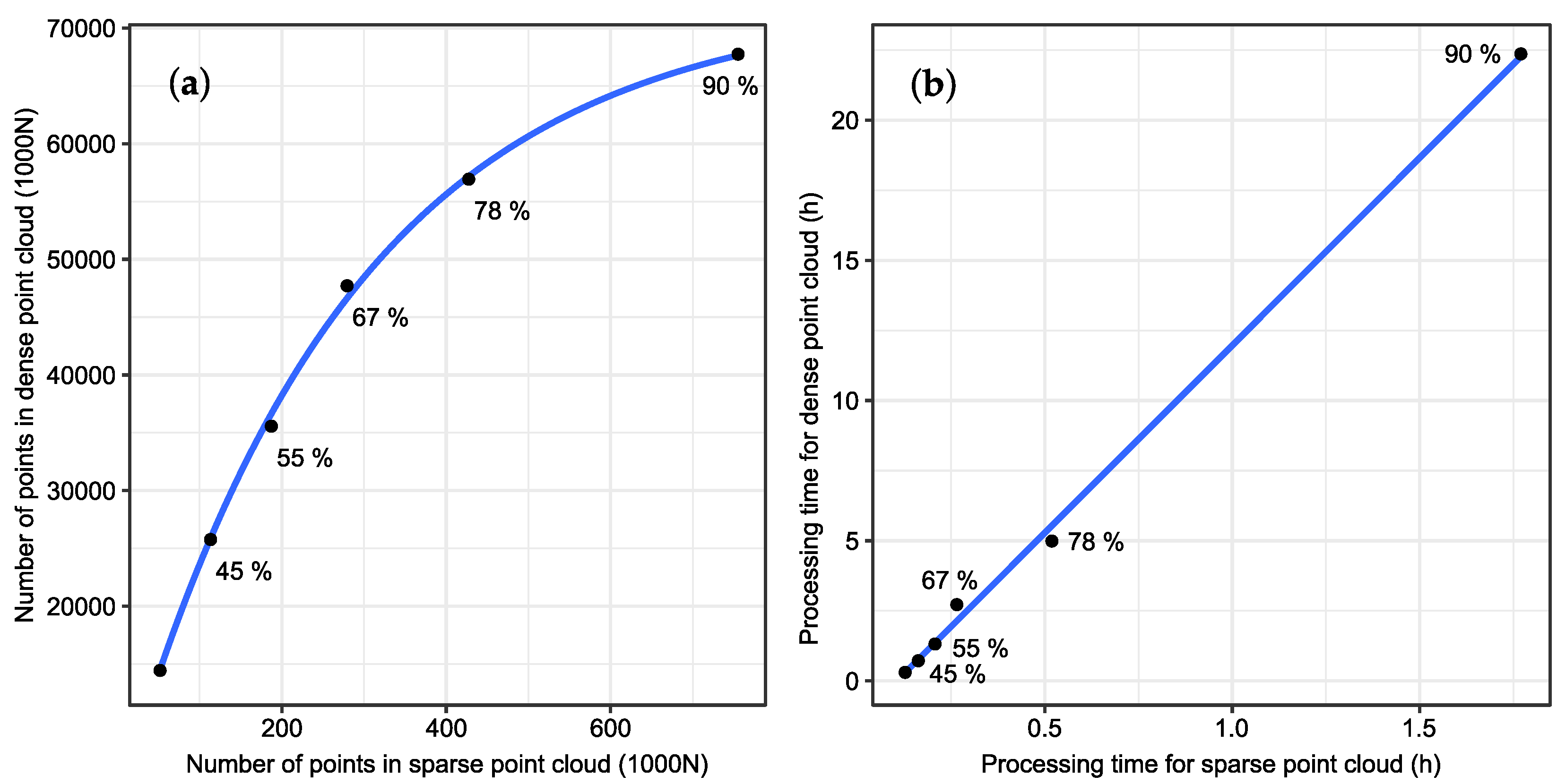
3.1. Relation between Sparse and Dense Point Clouds

The number of points in the dense point cloud regressed over the number of points in the sparse point cloud (Figure 4a) showed a tight positive relation, which approached a horizontal asymptote. This means that higher tie point numbers in the sparse point cloud will lead to higher detail in the dense point cloud reconstruction, which supports our choice of selecting tie numbers as a surrogate for reconstruction detail. The pattern seems to follow a rate of diminishing returns. This means that when the dense point cloud numbers approach the asymptote, additional sparse tie point numbers will only increase the dense point cloud numbers to a relatively small degree.

The relation of sparse and dense point processing time is linear (Figure 4b). In our case the dense point cloud reconstruction took about 13.4 times as long as the sparse point cloud reconstruction. This tight linear relationship shows that the dense point cloud reconstruction can easily be estimated from the sparse point cloud reconstruction time and was thus not further pursued in this article.

The influence of tie point numbers on the final reconstruction detail in the dense point cloud is illustrated in Figure 5. While no substantial advantage of higher tie point numbers was detected in the conifers, the deciduous tree showed clear reconstruction gaps when lower tie point numbers were used to reconstruct the dense point cloud as can be seen on the lower left and lower right part of Figure 5b.

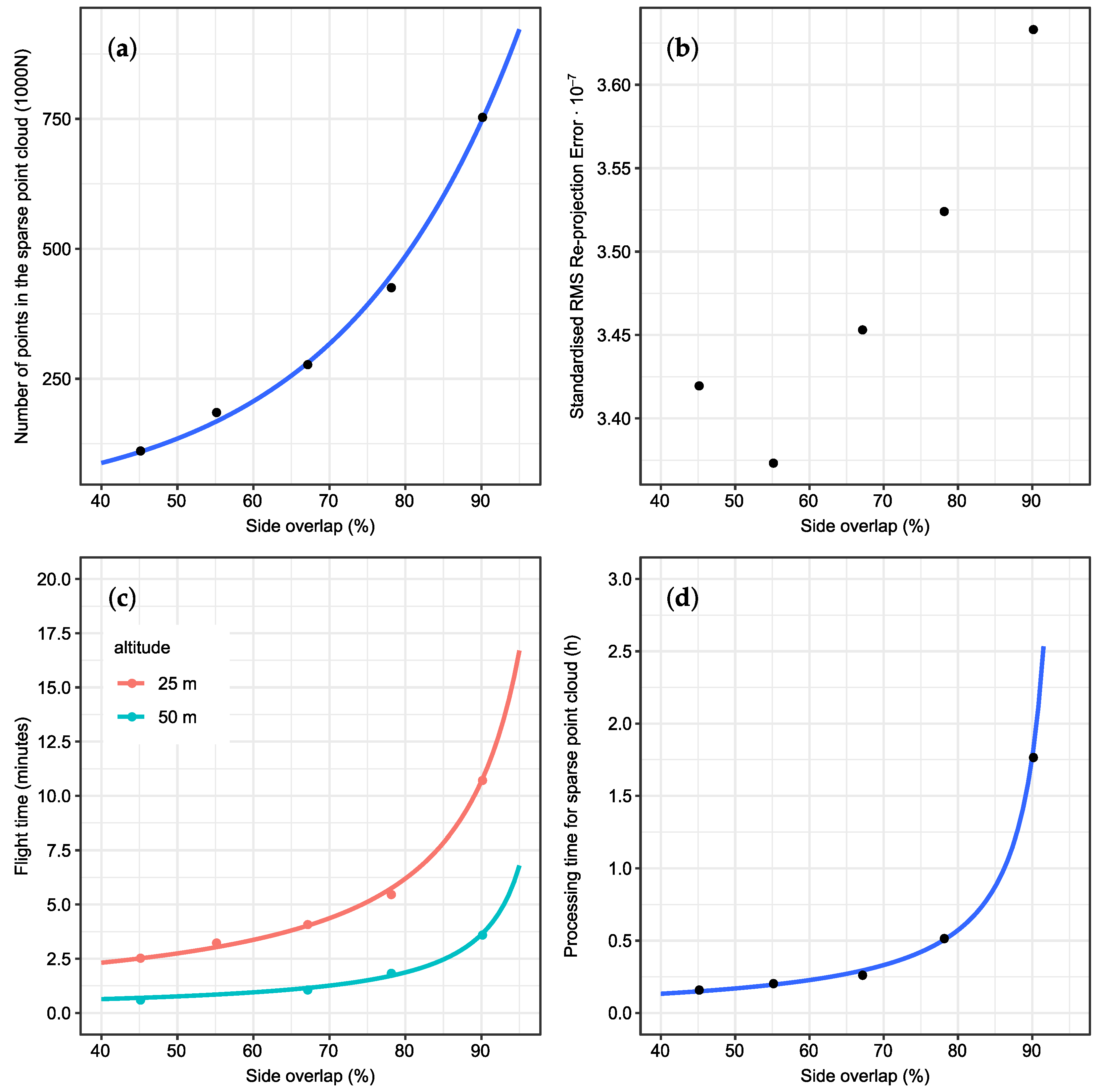
3.2. Influence of Side Overlap

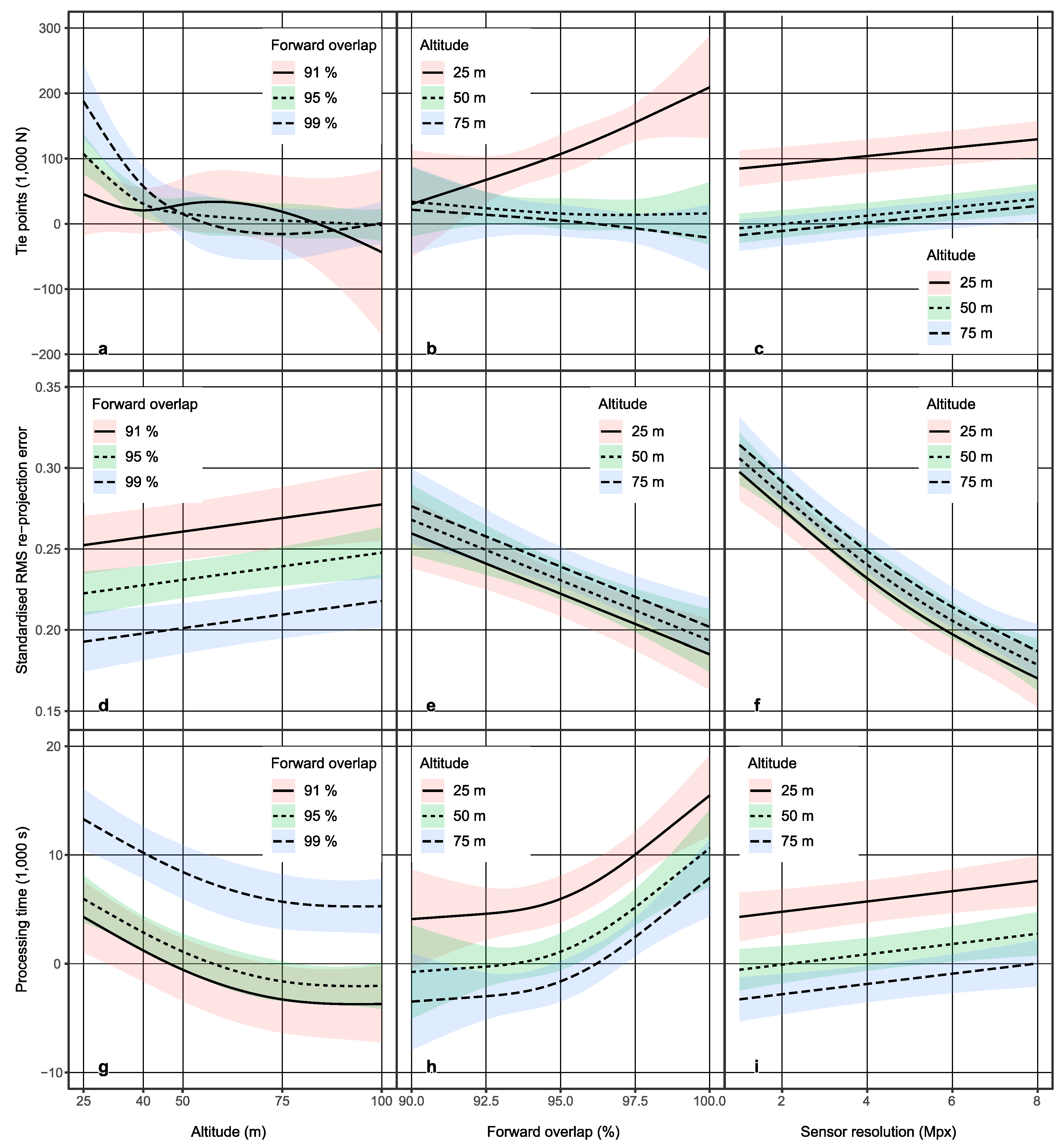
The influence of side overlap on reconstruction detail, reconstruction accuracy, flight time, and processing time was analysed (Figure 6a–d). Results indicate that tie point numbers increased exponentially with increasing side overlap (Figure 6a). The reconstruction accuracy increased with lower side overlaps, showed a minimum at 55% and decreased again at lower side overlap values (Figure 6b). Flight time increased with hyperbolic growth with higher side overlap rates (Figure 6c), as did processing time (Figure 6d). The optimum side overlap rate with regards to processing efficiency (s/1000 tie points) was at 67% for the sparse point cloud.

It is important to mention that the reconstruction was not fully completed at a side overlap of smaller than 55%. Thus, the side overlap of 67% was the smallest side overlap rate that had a complete reconstruction. Interestingly, the incomplete parts of the reconstruction always started on the edges.

3.3. Models

The initial analyses revealed strong interactions between altitude and forward image overlap on identified tie point numbers, which was addressed with a bivariate spline. A spline modelling on a full-rank data matrix was conducted for the three variables, namely altitude, forward overlap and sensor resolution.

The model for the tie point numbers was:

$$tps={\beta }_0+o_{forward}+res+f_1(alt)+f_2(alt,o_{forward})+ϵ,$$

(5)

where $tps$ is the tie point number in the sparse point cloud, ${\beta }_0$ is the model intercept, $f_1$ is a cubic spline function and $f_2$ is a bivariate tensor spline for the interaction of altitude and forward overlap, while $ϵ$ is the residual error. The dimensions of the bases used to represent the smooth term for the spline smoothers [34] were carefully selected and reduced to a maximum that prevented irrational spline oscillation.

The model for the root mean square re-projection error was:

$$RMSRE={\beta }_0+o_{forward}+f_1(res)+ϵ,$$

(6)

where RMSRE is the root mean square re-projection error, ${\beta }_0$ is the model intercept, $f_1$ is a cubic spline function, and $ϵ$ is the residual error.

The model for the processing time was:

$$t_{processing}={\beta }_0+res+f_1(alt)+f_2(o_{forward})+ϵ,$$

(7)

where $t_{processing}$ is the processing time for the sparse point cloud (s), ${\beta }_0$ being the model intercept, $f_1$ and $f_2$ are cubic spline functions, $ϵ$ is the residual error.

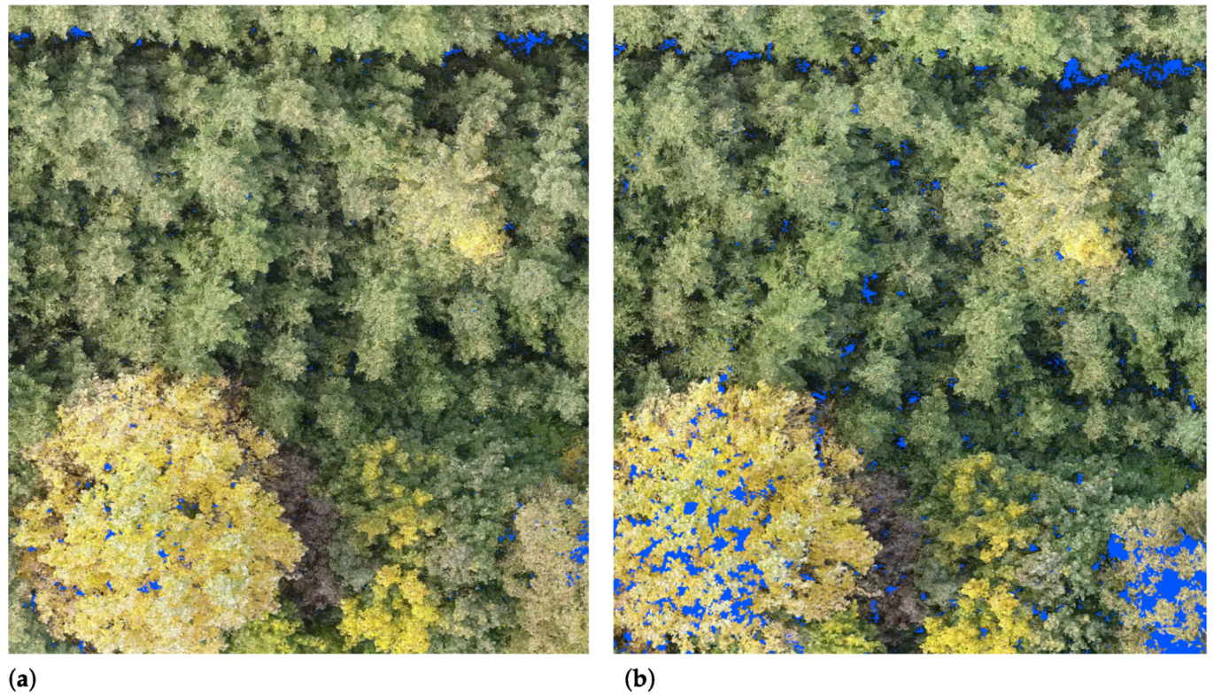
3.4. Reconstruction Details

Data visualisation and modelling showed that 3D reconstruction detail, as expressed by the identified tie points, was mainly dependent on altitude (and hence spatial resolution on the ground) and forward image overlap, but was to a lesser degree also influenced by sensor resolution. All factors were related in clearly different patterns to tie point numbers.

Altitude influenced the number of tie points in a decreasing nonlinear fashion (Figure 7a), levelling off at about 50 m. Higher forward overlaps linearly increased the number of tie points, but only at very low altitudes. At altitudes of 50 m or higher, the increasing forward overlap had no or a slightly negative effect on tie point numbers. Strong interaction effects existed between altitude and forward overlap, as these impact the quality of 3D image reconstruction (Figure 8). Higher image overlaps only contributed significantly to reconstruction quality at low altitudes. At lower altitudes (25 m above ground and about 15 m above the tree canopy), the effect of forward overlap was maximised at the highest overlap rates of 98.8% (Figure 7b). Sensor resolution contributed positively, but in a near-linear pattern (Figure 7c).

A closer analysis of the empirical data, where a flight at 25 m was compared with a flight at 50 m for the effect of forward overlap on tie point numbers, more clearly revealed this pattern (Figure 9). While high forward overlaps beyond 92% did not increase the number of tie points at 50 m altitude, they clearly increased tie point numbers at 25 m. The increase was substantial with nearly 20 times more tie points occurring at 25 m. This was attributed to the higher spatial resolutions, due to closer sensor-object ranges, resulting in an increase in tree details being captured. However, in order to rule out a possible effect of spatial resolution on the ground, the images of the flight at 25 m were re-rendered to the same spatial resolution as the flight at 50 m. The resulting regression line (green line in Figure 9) shows that at low altitudes the tie point numbers were still drastically increased (2–10 fold), even when the spatial resolution was resampled to the same at both altitudes.

3.5. Reconstruction Precision

The SRMSRE exhibited a different variable influence when compared to the tie points assessment. There was a negative linear effect of altitude on the precision of the image reconstruction. Higher altitudes slightly increased the error (Figure 7d). Forward overlap showed a linear negative relationship, which means that higher overlaps lead to significantly smaller errors (Figure 7e). Higher sensor resolutions had a clearly significant negative influence, but the pattern is nonlinear, indicating that increasing sensor resolution does not decrease the error proportionally (Figure 7f). The results show that sensor resolution and forward overlap have the strongest influence on the SRMSRE.

3.6. Processing Time of the Sparse Reconstruction

Processing time of the tie points in the sparse point cloud included the photo alignment procedure in Agisoft PhotoScan. It was influenced by altitude and in the same magnitude by forward overlap, both of which determine the number of images acquired by the drone. The relationship showed a negative degressive nonlinear pattern, levelling off at about 75 m; Reconstructions with 99% forward overlap required a significantly longer time to be processed than the same flight with 95% or 91% forward overlap (Figure 7g). Forward overlap contributed to processing time in a positive progressive exponential pattern, with a strong increase from 95% overlap onwards. Twenty-five meters showed significantly higher processing times than 50 m altitude (Figure 7h). Sensor resolution influenced processing times in a positive linear pattern, with 25 m altitude significantly higher than 50 m or 75 m (Figure 7i). The result suggests that processing time is to a much higher degree dependent on the number of images, as opposed to sensor resolution. While the most detail can be gained by increasing forward overlap and spatial resolution on the ground, sensor resolution has the greatest impact on the accuracy of the image reconstruction.

4. Discussion

4.1. Major Findings

This study is one of the few systematic analyses of the influence of different flight and sensor parameters on multi-view image reconstruction quality and efficiency of drone-based sensing in a forest environment. It provides novel information for drone flight planning and could in theory be upscaled to larger manned acquisition platforms and be used for photogrammetric benchmarking. The developed method for extracting images from video proved to be versatile in controlling the forward overlap and for achieving extraordinary overlaps of up to 98.8%, without a major loss in efficiency (flight time). Our study is also, to our knowledge, the first to be based on video data, instead of still images.

An important finding was that the side overlap of the images was a major driver of flight time and processing time. Higher side overlaps, when combined with high forward overlaps increased the reconstruction detail but were detrimental to the reconstruction accuracy. However, altitude had a stronger effect on flight time.

Drone flights at low altitudes dramatically increased the number of tie points and thus reconstruction detail. This was particularly true when low altitudes were combined with high forward overlaps. The question now arises whether similar tie point numbers could have been achieved using higher sensor resolutions at higher altitudes, which would have increased the flight efficiency. Our results indicate that it will be hard to compensate for the level of reconstruction detail with higher sensor resolutions, which we attributed to a changed image geometry at low altitudes, where more of the tree silhouettes are visible. Possible explanations for the observed nonlinear increase of identified tie points with decreasing altitude are that (i) more details can be detected with higher object resolutions, (ii) the inherent perspective distortion leads to higher tie point detection at tree silhouettes, and (iii) the lower relative flight speed (altitude-to-velocity ratio). Our results indicate that it is not merely a matter of higher object resolution. A further investigation of these effects would be desirable to better understand their impact.

4.2. Comparison to Findings by Other Authors

Our findings are in contrast to the traditional remote sensing paradigm that higher altitudes are advantageous because they minimise perspective distortion. Our finding of the positive compounding effect of low altitudes and high forward overlaps on reconstruction detail has not, to our knowledge, been reported. The reasons might be that other studies have not explored that specific parameter space and/or have applied different metrics for measuring the success of the MVG reconstruction. There are, however, some references that point towards similar outcomes as we have found in our study.

Torres-Sánchez et al. [37] mentioned an optimum reconstruction solution at a flight height of 100 m and at 95% overlap for olive orchards, in terms of cost-benefit relation. However, they achieved higher accuracies at 97% overlap but did not test altitudes that brought the drone close to the tree canopies. Their accuracy criterion was an MVG-derived crown volume compared to a manually-measured crown volume. Frey et al. [32] for example showed positive effects of off-nadir imagery for tree reconstruction. The authors tested forward overlap ratios ranging from 75% to 95% for many stands, also mentioning that the most complete reconstruction results, based on surface coverage, were achieved with an image overlap of 95% and higher. This is in line with our findings, but the higher overlaps (>95%) we tested yielded additional gains in tie point numbers at low altitudes. Finally, Dandois et al. [31] compared airborne LiDAR with MVG, based on top-of-canopy heights of temperate deciduous forests as a metric, and flew with forward overlaps of up to 96%. They also pointed out that maximising forward overlap is essential to minimise the error in canopy height estimation.

4.3. Reasonable Ranges for Flight Parameters

It is challenging to provide optimum values for flight and sensor parameters since each combination of drone, sensor, and post-processing system will be vastly different and must be individually assessed. Nonetheless, we here attempt to provide a range of reasonable parameter values as a guideline, based on our results.

We contend that relatively low altitudes (15–30 m above canopy in our case) in combination with the highest possible forward overlap are advisable, in order to harness the compound effect on reconstruction detail. This also affects the reconstruction accuracy positively. Should processing time pose a significant constraint, a forward overlap of 95% should be set as a limit. A clearly nonlinear increase impacted the computing time at higher forward overlap rates. However, we can expect that with faster processors, access to massive multi-processing facilities and software optimised for parallel computing, processing time will be less of a constraint in the future.

In terms of the side overlap, the 90% overlap chosen for this scientific study was clearly on the high side. Similarly high reconstruction details could have been achieved along with higher pixel accuracies at side overlap rates in the range of 70% or 80%. Based on our study in combination with very high forward overlaps, side overlaps of around 70% were clearly the most efficient in terms of flight time, area coverage and processing time. However, it must be stated that the influence of altitude on the square meters imaged per second of drone flight is substantially larger than the effect of the side overlap rate (Figure 10).

Higher optical sensor resolutions were clearly better in terms of reconstruction detail, but mainly in terms of reconstruction accuracy, while only impacting processing times in a linear fashion. Due to the unexpectedly low impact on processing time, the highest possible sensor resolution should be used. However, higher sensor resolutions were not able to achieve comparable gains in reconstruction detail, when compared with the compound effect of low altitude and high forward overlap. It must be stated that lower altitudes also required a reduced drone speed to avoid motion blur (Figure 3) and hence reduced drone endurance and area covered with one battery load. The covered area with our configuration was limited to 1.5 ha with one battery. However, this only constrained the efficiency, not the total area covered, as the flight planning software allows the flight mission to be continued after a battery change.

4.4. Contextualisation of Our Results and Future Opportunities

The focus of this study was to assess flight parameters that can be directly controlled by the flight operator, and their quantitative impact on image reconstruction. It was not in the scope to test further influences on the MVG reconstruction, such as wind, cloud cover, and illumination conditions, since these have been addressed in previous studies. For example, Dandois et al. [31] described the relationship between weather conditions and errors in reconstruction. They found that the effect of wind speed was negligible, while illumination conditions (cloud cover) influenced reconstruction quality, but could be compensated for by preprocessing. As weather conditions can hardly be controlled, we chose weather conditions that were within the optimum range for our flights. As such, the flights in this study were conducted under sunny conditions around solar noon, with minimum wind speeds.

We tested the MVG approach with only PhotoScan, a popular commercial software. The implemented SIFT-like MVG algorithm might perform differently to alternative algorithms which should be tested in the future [31]. It is important to mention in this context that PhotoScan filters tie points via a proprietary algorithm, which removes tie points of minor quality automatically. However, the fact that the software has been successfully used in previous studies [20,31,32,37] constitutes a solid baseline for comparison. Other drone configurations, other more variable forest stands or a different software, featuring a different MVG algorithm, might lead to different results.

With our choice to use the tie points, instead of tree variables such as crown volume and height, we concentrated on the MVG reconstruction rather than taking the next processing step into forest inventory measurements, which might have depended on further variables derived from the dense point cloud.

Another strength of our study is arguably the use of a video stream, instead of still images, to generate image-to-image reconstruction solutions. It enabled us to fly at a constant speed and derive high forward overlap ratios of up to 98.8%. No GNSS coordinates were used for the reconstruction and the reconstruction process had to rely only on image features and the calculation of camera positions in PhotoScan. An even better reconstruction success could be expected by additionally using GNSS coordinates.

We regard the systematic nature of our study as an advantage, since we achieved a full rank design regarding our major tested factors altitude, forward overlap, and processing time, and were thus able to conduct rigorous statistical modelling with our data. The high effort in this systematic setup limited the study to one stand. The fact that the sample stand was a young mono-layered stand dominated by conifers definitely provided a rather homogeneous forest structure. On the other hand, stands consisting largely of deciduous trees provide opportunities of flying during either the vegetative period or when the leaves are off. While the latter would increase the penetration into the crown zone as shown by Frey et al. [32], it could also lead to new or different challenges in the reconstruction. In multi-layered stands with a dense upper canopy, it can only be expected that the upper canopy layer would be reconstructed properly when flown in the vegetative period. To cover different forest types, the impact of these variables should be tested in future investigations.

5. Conclusions

In summary, we arrived at a number of conclusions:

• The processing of video stream data in the MVG reconstruction proved to be successful and efficient. It facilitated a constant flight speed and enabled high forward overlap rates.
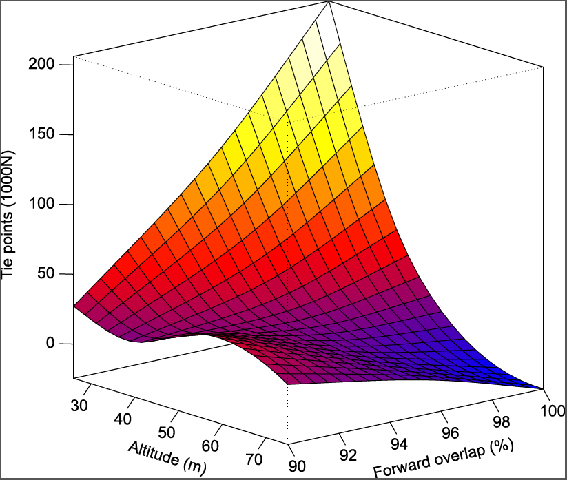
• Low altitudes of 15–30 m above canopy, in combination with high forward overlap rates of close to 99%, led to the best reconstruction detail and accuracy. High detail in object geometry was identified as the most likely cause of this effect. This compound effect could not easily be recreated with an increased sensor resolution at higher altitudes, since the sensor resolution was only linear, while the compound effect was nonlinear.
• The nonlinear effects of forward overlap and altitude on processing time might pose a constraint on using forward overlap rates higher than 95%, if processing time is the main limitation.
• In contrast to the forward overlap, the side overlap showed an optimum in reconstruction accuracy in a range between 50% and 70%.
• First reasonable ranges for flight parameter selection have been provided based on this study.

References

1. Goodbody, T.R.; Coops, N.C.; Marshall, P.L.; Tompalski, P.; Crawford, P. Unmanned aerial systems for precision forest inventory purposes: A review and case study. For. Chron. 2017, 93, 71–81. [Google Scholar] [CrossRef] [Green Version]
2. Torresan, C.; Berton, A.; Carotenuto, F.; Filippo Di Gennaro, S.; Gioli, B.; Matese, A.; Miglietta, F.; Vagnoli, C.; Zaldei, A.; Wallace, L. Forestry applications of UAVs in Europe: A review. Int. J. Remote Sens. 2017, 38, 2427–2447. [Google Scholar] [CrossRef]
3. International Union of Forest Research Organizations. Scientific Summary No. 19. Available online: https://www.iufro.org/publications/summaries/article/2006/05/31/scientific-summary-no-19/ (accessed on 1 March 2019).
4. Seifert, T.; Klemmt, H.J.; Seifert, S.; Kunneke, A.; Wessels, C.B. Integrating terrestrial laser scanning based inventory with sawing simulation. In Developments in Precision Forestry Since 2006, Proceedings of the International Precision Forestry Symposium, Stellenbosch University, Stellenbosch, South Africa, 1–3 March 2010; Ackerman, P.A., Ham, H., Lu, C., Eds.; Department of Forest and Wood Science: Stellenbosch, South Africa, 2010. [Google Scholar]
5. Ducey, M.J.; Astrup, R.; Seifert, S.; Pretzsch, H.; Larson, B.C.; Coates, K.D. Comparison of Forest Attributes Derived from Two Terrestrial Lidar Systems. Photogramm. Eng. Remote Sens. 2013, 79, 245–257. [Google Scholar] [CrossRef]
6. Holopainen, M.; Vastaranta, M.; Hyyppä, J. Outlook for the Next Generation’s Precision Forestry in Finland. Forests 2014, 5, 1682–1694. [Google Scholar] [CrossRef]
7. Kunneke, A.; van Aardt, J.; Roberts, W.; Seifert, T. Localisation of Biomass Potentials. In Bioenergy from Wood: Sustainable Production in the Tropics; Seifert, T., Ed.; Springer: Dordrecht, The Netherlands, 2014; pp. 11–41. [Google Scholar] [CrossRef]
8. Salamí, E.; Barrado, C.; Pastor, E. UAV Flight Experiments Applied to the Remote Sensing of Vegetated Areas. Remote Sens. 2014, 6, 11051–11081. [Google Scholar] [CrossRef] [Green Version]
9. Sauerbier, M.; Siegrist, E.; Eisenbeiss, H.; Demir, N. The Practical Application of UAV-Based Photogrammetry under Economic Aspects. ISPRS Int. Arch. Photogramm. Remote Sens. Spat. Inf. Sci. 2011, 38, 45–50. [Google Scholar] [CrossRef]
10. Wallace, L.; Lucieer, A.; Watson, C.; Turner, D. Development of a UAV-LiDAR System with Application to Forest Inventory. Remote Sens. 2012, 4, 1519–1543. [Google Scholar] [CrossRef] [Green Version]
11. Watts, A.C.; Ambrosia, V.G.; Hinkley, E.A. Unmanned Aircraft Systems in Remote Sensing and Scientific Research: Classification and Considerations of Use. Remote Sens. 2012, 4, 1671–1692. [Google Scholar] [CrossRef] [Green Version]
12. Baltsavias, E.; Gruen, A.; Eisenbeiss, H.; Zhang, L.; Waser, L. High-quality image matching and automated generation of 3D tree models. Int. J. Remote Sens. 2008, 29, 1243–1259. [Google Scholar] [CrossRef]
13. Leberl, F.; Irschara, A.; Pock, T.; Meixner, P.; Gruber, M.; Scholz, S.; Wiechert, A. Point Clouds. Photogramm. Eng. Remote Sens. 2010, 76, 1123–1134. [Google Scholar] [CrossRef]
14. White, J.C.; Wulder, M.A.; Vastaranta, M.; Coops, N.C.; Pitt, D.; Woods, M. The Utility of Image-Based Point Clouds for Forest Inventory: A Comparison with Airborne Laser Scanning. Forests 2013, 4, 518–536. [Google Scholar] [CrossRef] [Green Version]
15. Hardin, P.J.; Jensen, R.R. Small-Scale Unmanned Aerial Vehicles in Environmental Remote Sensing: Challenges and Opportunities. GIScience Remote Sens. 2011, 48, 99–111. [Google Scholar] [CrossRef]
16. Whitehead, K.; Hugenholtz, C.H. Remote sensing of the environment with small unmanned aircraft systems (UASs), part 1: A review of progress and challenges. J. Unmanned Veh. Syst. 2014, 2, 69–85. [Google Scholar] [CrossRef]
17. Fritz, A.; Kattenborn, T.; Koch, B. UAV-based photogrammetric point clouds—Tree stem mapping in open stands in comparison to terrestrial laser scanner point clouds. ISPRS Int. Arch. Photogramm. Remote Sens. Spat. Inf. Sci. 2013, 141–146. [Google Scholar] [CrossRef]
18. Nesbit, P.R.; Hugenholtz, C.H. Enhancing UAV–SfM 3D Model Accuracy in High-Relief Landscapes by Incorporating Oblique Images. Remote Sens. 2019, 11, 239. [Google Scholar] [CrossRef]
19. Jaakkola, A.; Hyyppä, J.; Kukko, A.; Yu, X.; Kaartinen, H.; Lehtomäki, M.; Lin, Y. A low-cost multi-sensoral mobile mapping system and its feasibility for tree measurements. ISPRS J. Photogramm. Remote Sens. 2010, 65, 514–522. [Google Scholar] [CrossRef]
20. Dandois, J.P.; Ellis, E.C. High spatial resolution three-dimensional mapping of vegetation spectral dynamics using computer vision. Remote Sens. Environ. 2013, 136, 259–276. [Google Scholar] [CrossRef] [Green Version]
21. Wallace, L.; Lucieer, A.; Malenovský, Z.; Turner, D.; Vopěnka, P. Assessment of Forest Structure Using Two UAV Techniques: A Comparison of Airborne Laser Scanning and Structure from Motion (SfM) Point Clouds. Forests 2016, 7, 62. [Google Scholar] [CrossRef]
22. Garber, S.M.; Temesgen, H.; Monleon, V.J.; Hann, D.W. Effects of height imputation strategies on stand volume estimation. Can. J. For. Res. 2009, 39, 681–690. [Google Scholar] [CrossRef]
23. Seifert, T.; Seifert, S. Modelling and Simulation of Tree Biomass. In Bioenergy from Wood: Sustainable Production in the Tropics; Seifert, T., Ed.; Springer: Dordrecht, The Netherlands, 2014; pp. 43–65. [Google Scholar] [CrossRef]
24. Mensah, S.; Pienaar, O.L.; Kunneke, A.; du Toit, B.; Seydack, A.; Uhl, E.; Pretzsch, H.; Seifert, T. Height–Diameter allometry in South Africa’s indigenous high forests: Assessing generic models performance and function forms. For. Ecol. Manag. 2018, 410, 1–11. [Google Scholar] [CrossRef]
25. Pekin, B.K.; Jung, J.; Villanueva-Rivera, L.J.; Pijanowski, B.C.; Ahumada, J.A. Modeling acoustic diversity using soundscape recordings and LIDAR-derived metrics of vertical forest structure in a neotropical rainforest. Landsc. Ecol. 2012, 27, 1513–1522. [Google Scholar] [CrossRef]
26. Müller, J.; Brandl, R.; Buchner, J.; Pretzsch, H.; Seifert, S.; Strätz, C.; Veith, M.; Fenton, B. From ground to above canopy—Bat activity in mature forests is driven by vegetation density and height. For. Ecol. Manag. 2013, 306, 179–184. [Google Scholar] [CrossRef]
27. Seifert, T.; Seifert, S.; Seydack, A.; Durrheim, G.; Gadow, K.V. Competition effects in an afrotemperate forest. For. Ecosyst. 2014, 1, 13. [Google Scholar] [CrossRef]
28. Goodbody, T.R.H.; Coops, N.C.; White, J.C. Digital Aerial Photogrammetry for Updating Area-Based Forest Inventories: A Review of Opportunities, Challenges, and Future Directions. Curr. For. Rep. 2019, 5, 55–75. [Google Scholar] [CrossRef] [Green Version]
29. Falkner, E.; Morgan, D. Aerial Mapping: Methods and Applications, 2nd ed.; CRC Press: Boca Raton, FL, USA, 2002. [Google Scholar]
30. Leachtenauer, J.C.; Driggers, R.G. Surveillance and Reconnaissance Imaging Systems: Modeling and Performance Prediction; Artech House: Norwood, MA, USA, 2001. [Google Scholar]
31. Dandois, J.P.; Olano, M.; Ellis, E.C. Optimal Altitude, Overlap, and Weather Conditions for Computer Vision UAV Estimates of Forest Structure. Remote Sens. 2015, 7, 13895–13920. [Google Scholar] [CrossRef] [Green Version]
32. Frey, J.; Kovach, K.; Stemmler, S.; Koch, B. UAV Photogrammetry of Forests as a Vulnerable Process. A Sensitivity Analysis for a Structure from Motion RGB-Image Pipeline. Remote Sens. 2018, 10, 912. [Google Scholar] [CrossRef]
33. CloudCompare Team. CloudCompare: 3D Point Cloud and Mesh Processing Software. Available online: http://www.cloudcompare.org/ (accessed on 1 March 2019).
34. Wood, S.N. Fast stable restricted maximum likelihood and marginal likelihood estimation of semiparametric generalized linear models. J. R. Stat. Soc. Ser. B Stat. Methodol. 2011, 73, 3–36. [Google Scholar] [CrossRef]
35. Zuur, A.; Ieno, E.N.; Walker, N.; Saveiliev, A.A.; Smith, G.M. Mixed Effects Models and Extensions in Ecology with R; Springer: New York, NY, USA, 2009; ISBN 978-0-387-87457-9. [Google Scholar]
36. R Core Team. R: A Language and Environment for Statistical Computing; R Foundation for Statistical Computing: Vienna, Austria, 2018. [Google Scholar]
37. Torres-Sánchez, J.; López-Granados, F.; Borra-Serrano, I.; Peña, J.M. Assessing UAV-collected image overlap influence on computation time and digital surface model accuracy in olive orchards. Precis. Agric. 2018, 19, 115–133. [Google Scholar] [CrossRef]
Figure 1. Different parameters in drone flights. The outer box represents the target variables, while the inner box shows the parameters that can be directly influenced by the mission planner and derivatives of those parameters.
Remotesensing 11 01252 g001
Figure 2. The experimental stand seen on (a) a drone image and (b) ground level.
Remotesensing 11 01252 g002
Figure 3. Relationship of the altitude above ground and the corresponding speed that was calculated by the flight planning software. Equation and regression coefficients in Supplementary Table S1.
Remotesensing 11 01252 g003
Figure 4. Relationship between sparse reconstruction and dense reconstruction with regards to (a) point numbers and (b) processing times. The percent numbers indicate the side overlap that was used to vary the tie point numbers in the sparse point cloud. Equation and regression coefficients in Supplementary Table S1.
Remotesensing 11 01252 g004
Figure 5. Illustration of a section of the dense point cloud based on different tie point densities. (a) Dense reconstruction with a side overlap of 90% and 753,239 tie points in the sparse point cloud and 67,582,712 points in the total dense point cloud. (b) Dense reconstruction with a side overlap of 55% and 185,349 tie points in the sparse point cloud and 35,413,159 points in the total dense point cloud. Clearly visible are the missing points indicated by the blue background in the deciduous trees of the lower left and right corner of (b).
Remotesensing 11 01252 g005
Figure 6. Relationships between side overlap and (a) tie point numbers, (b) the SRMSRE, (c) the flight time, (d) the processing time for the sparse reconstruction. Equation and regression coefficients are in Supplementary Table S1.
Remotesensing 11 01252 g006
Figure 7. Trend observations for quality and efficiency parameters versus flight/sensor parameters. Displayed are the model predictions and a 95% prediction confidence interval ( p = 0.025 ).
Remotesensing 11 01252 g007
Figure 8. Generalised additive model (GAM) for identified tie point numbers in relation to drone altitude (above ground) and forward image overlap at a sensor resolution of 4 Mpx.
Remotesensing 11 01252 g008
Figure 9. The number of tie points plotted over the forward overlap. Linear regression lines were inserted to show the general reaction pattern. The different colours denote different altitudes (red and green for 25 m, blue for 50 m). The green line denotes for a rescaled flight at 25 m (GSD = 2.4 cm/px) with nearly the same ground resolution as the 50 m flight (2.2 cm/px). Equation and regression coefficients are in Supplementary Table S1.
Remotesensing 11 01252 g009
Figure 10. Influence of side overlap and altitude on area covered per time unit derived from Figure 6c. Equation and regression coefficients are in Supplementary Table S1.
Remotesensing 11 01252 g010