A Methodology to Monitor Urban Expansion and Green Space Change Using a Time Series of Multi-Sensor SPOT and Sentinel-2A Images

 ,
,
Abstract
1. Introduction
2. Materials and Methods
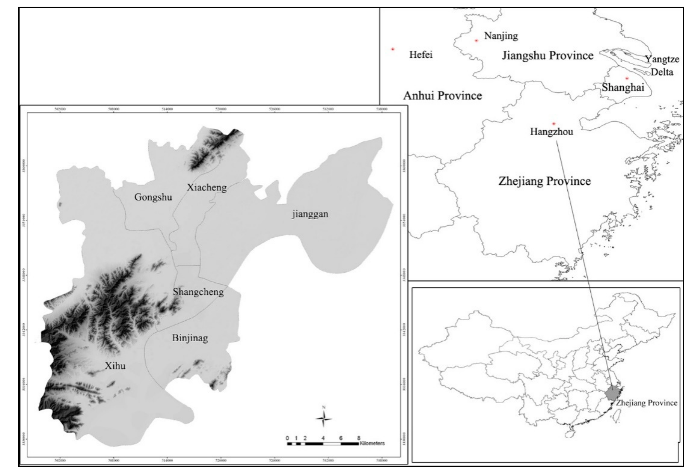
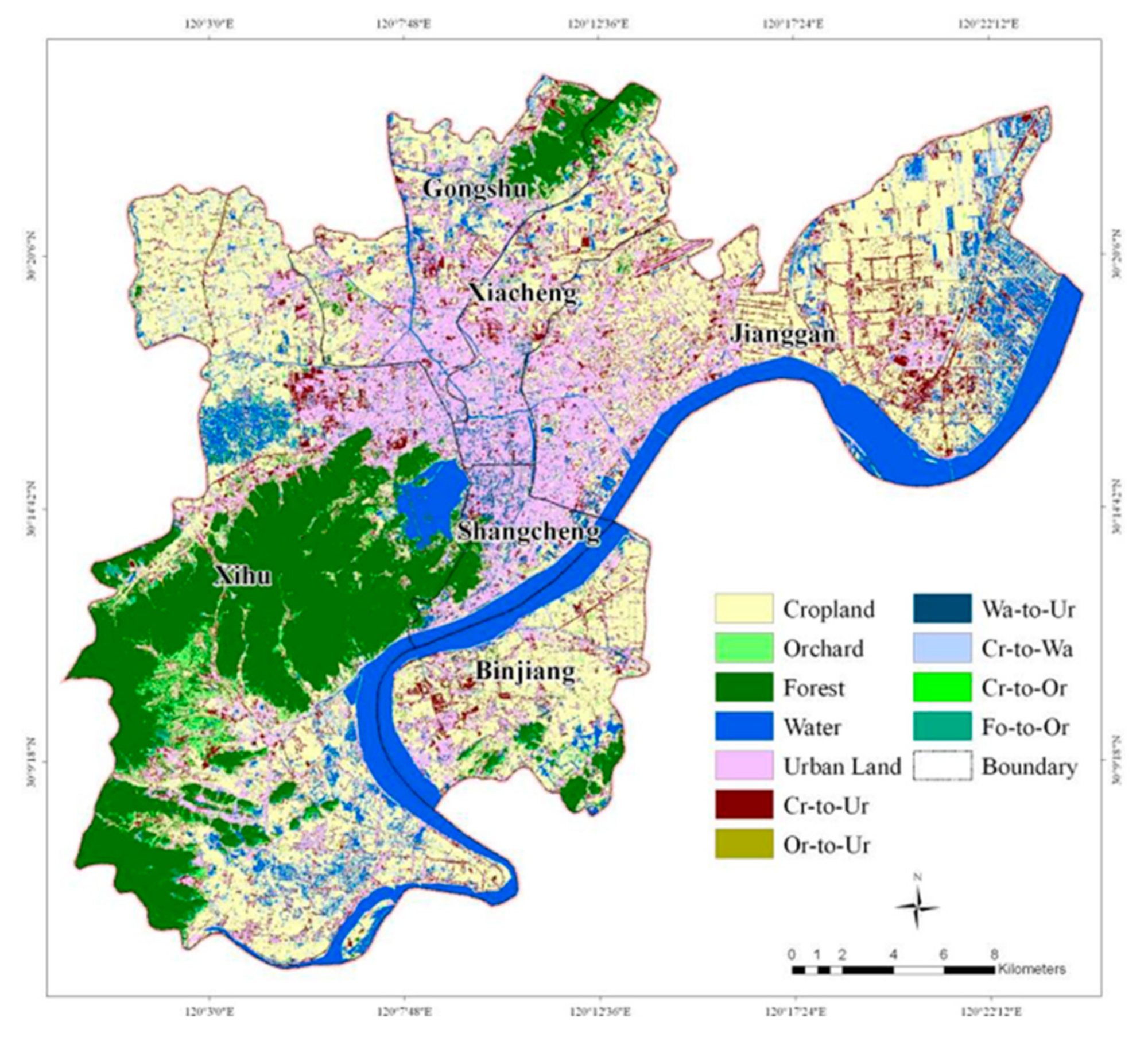
2.1. Study Area
2.2. Data Source
2.3. Methods
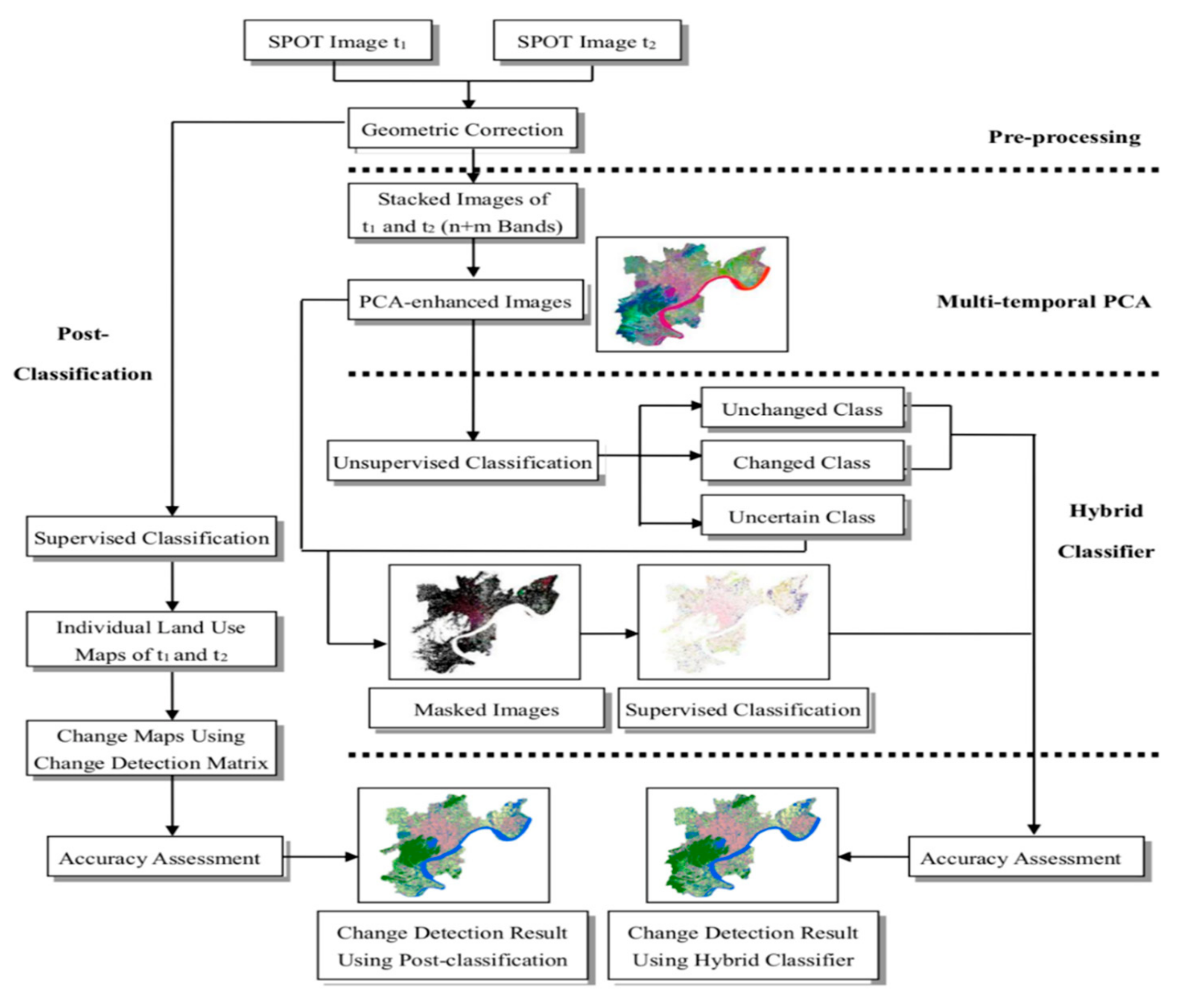
2.3.1. Flowchart
2.3.2. Pre-Processing
2.3.3. Multi-Date PCA for Enhancement Change Information
2.3.4. Hybrid Classifier for Extraction Change Information
2.3.5. Post-Classification Comparison Change Detection
2.3.6. Accuracy Assessment
3. Results
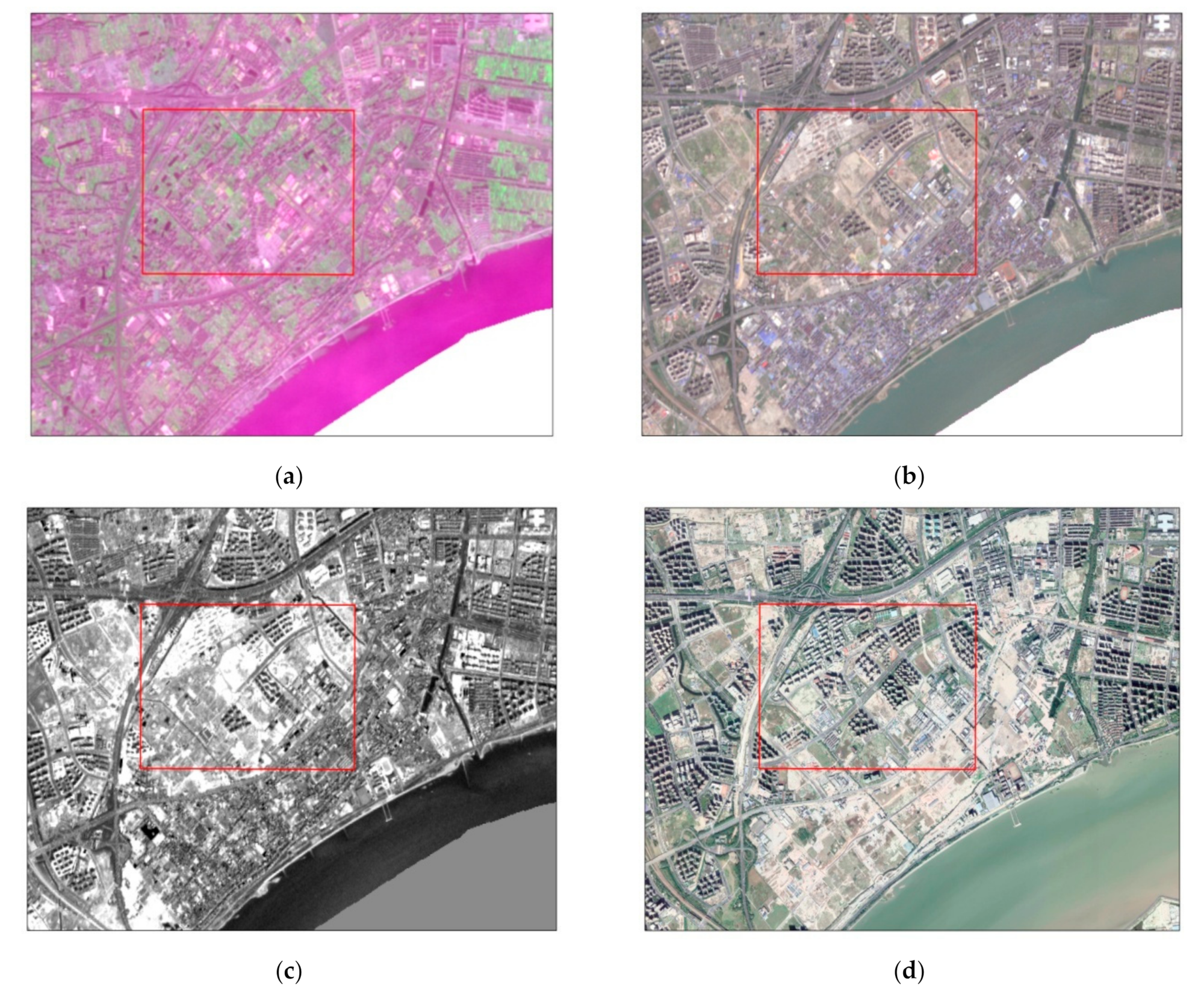
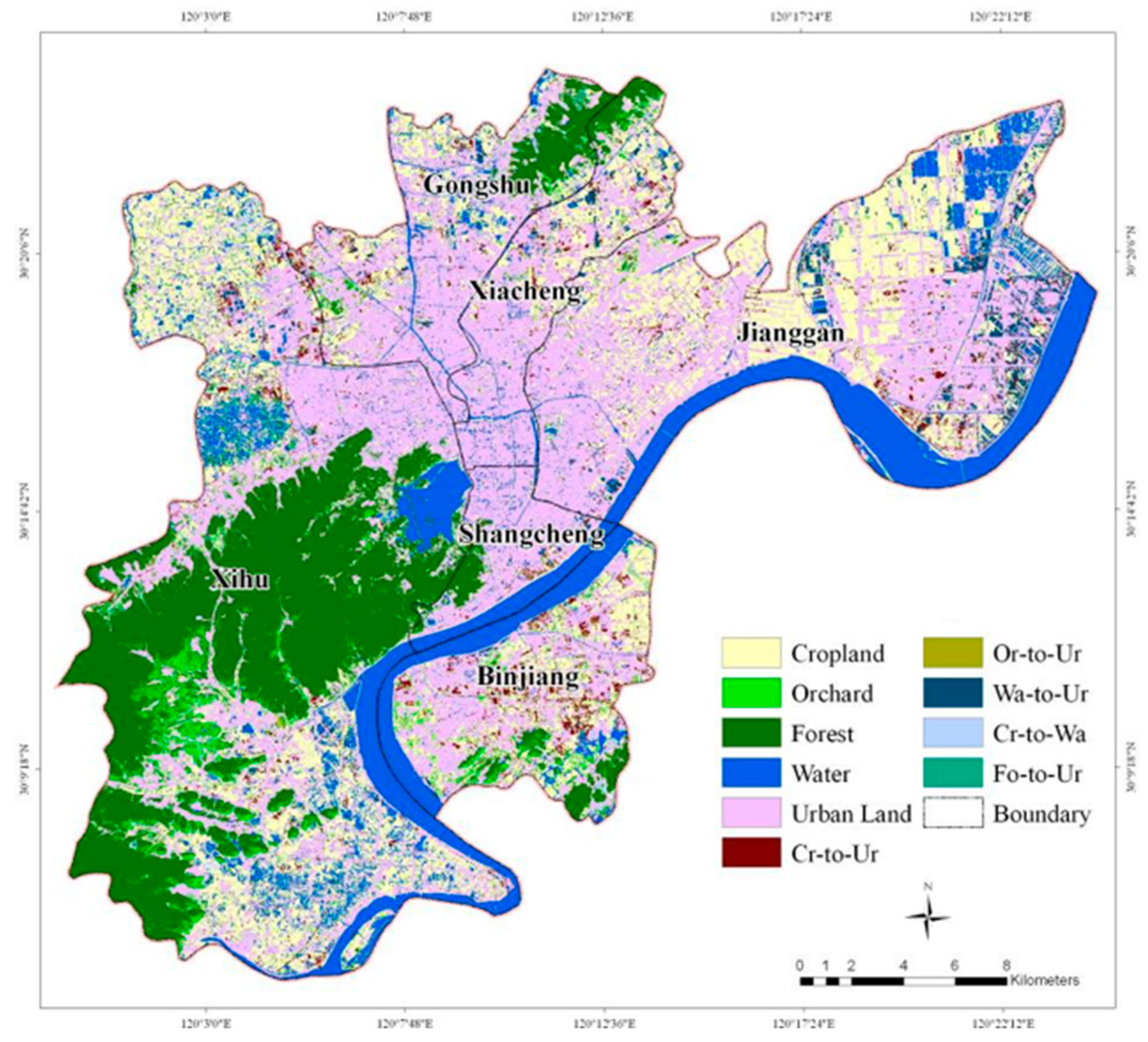
3.1. Urban Expansion and Green Space Change Detection for 2006–2016
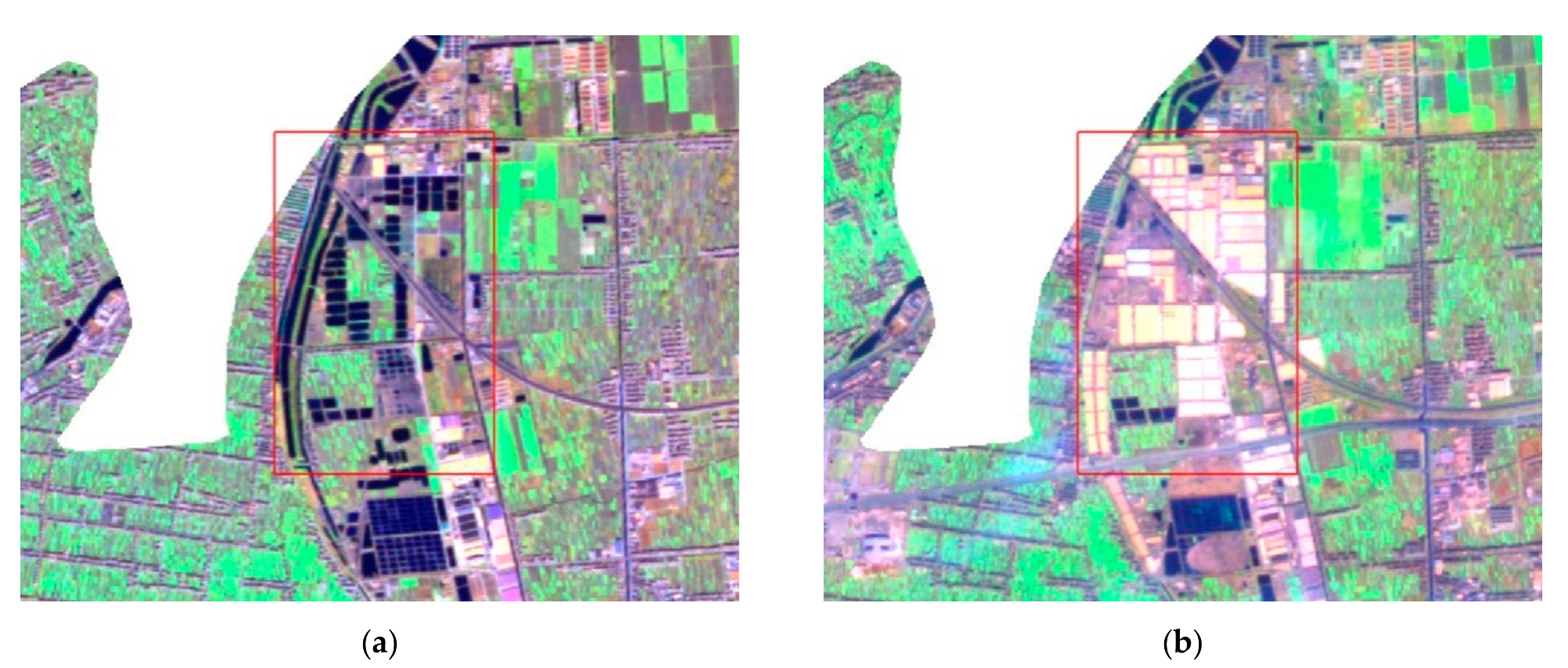
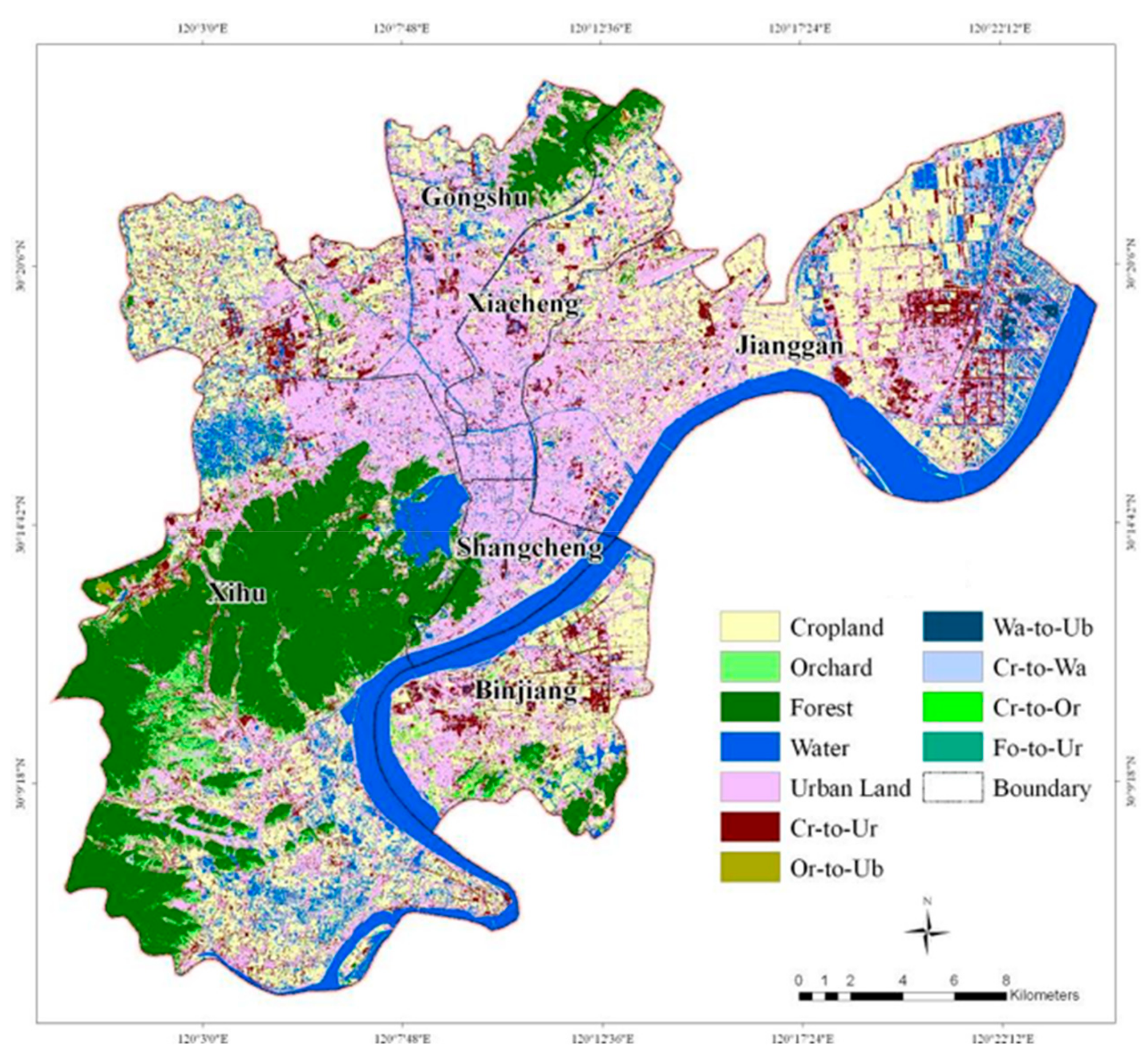
3.2. Urban Expansion and Green Space Change Detection for 2003–2006
3.3. Urban Expansion and Green Space Change Detection for 2000–2003
3.4. Urban Expansion and Green Space Change Detection for 1996–2000
4. Discussion
5. Conclusions
Author Contributions
Funding
Conflicts of Interest
References
- Chen, S.S.; Chen, L.F.; Liu, Q.H.; Li, X.; Tan, Q. Remote sensing and GIS-based integrated analysis of coastal changes and their environmental impacts in Lingding Bay, Pearl River Estuary, South China. Ocean Coast. Manag. 2005, 83, 65–83. [Google Scholar] [CrossRef]
- Ji, C.Y.; Liu, Q.H.; Sun, D.F.; Wang, S.; Lin, P.; Li, X.W. Monitoring urban expansion with remote sensing in china. Int. J. Remote Sens. 2001, 22, 1441–1455. [Google Scholar] [CrossRef]
- Weng, Q. A remote sensing? Gis evaluation of urban expansion and its impact on surface temperature in the zhujiang delta, china. Int. J. Remote Sens. 2001, 22, 1999–2014. [Google Scholar] [CrossRef]
- Yeh, A.G.O.; Li, X. Economic development and agricultural land loss in the pearl river delta, china. Habitat Int. 1999, 23, 373–390. [Google Scholar] [CrossRef]
- Yeh, A.G.O.; LI, X. Measurement and monitoring of urban sprawl in a rapidly growing region using entropy. Photogramm. Eng. Remote Sens. 2001, 63, 83–90. [Google Scholar]
- Dahmann, N.; Wolch, J.; Joassart-Marcelli, P.; Reynolds, K.; Jerrett, M. The active city? Disparities in provision of urban public recreation resources. Health Place 2010, 16, 431–445. [Google Scholar] [CrossRef]
- Sister, C.; Wolch, J.; Wilson, J. Got green? Addressing environmental justice in park provision. GeoJournal 2010, 75, 229–248. [Google Scholar] [CrossRef]
- Wolch, J.R.; Byrne, J.; Newell, J.P. Urban green space, public health, and environmental justice: The challenge of making cities ’just green enough’. Landsc. Urban Plan. 2014, 125, 234–244. [Google Scholar] [CrossRef]
- Zhou, X.; Wang, Y.C. Spatial–temporal dynamics of urban green space in response to rapid urbanization and greening policies. Landsc. Urban Plan. 2011, 100, 268–277. [Google Scholar] [CrossRef]
- Maas, J.; Verheij, R.A.; Groenewegen, P.P.; De, V.S.; Spreeuwenberg, P. Green space, urbanity, and health: How strong is the relation? J. Epidemiol. Community Health 2006, 60, 587–592. [Google Scholar] [CrossRef] [PubMed]
- Wan, L.; Ye, X.; Lee, J.; Lu, X.; Zheng, L.; Wu, K. Effects of urbanization on ecosystem service values in a mineral resource-based city. Habitat Int. 2015, 46, 54–63. [Google Scholar] [CrossRef]
- Awotwi, A.; Anornu, G.K.; Quaye-Ballard, J.; Annor, T.; Forkuo, E.K. Analysis of climate and anthropogenic impacts on runoff in the lower pra river basin of ghana. Heliyon 2017, 3. [Google Scholar] [CrossRef]
- Dimitrov, S.; Georgiev, G.; Georgieva, M.; Gluschkova, M.; Chepisheva, V.; Mirchev, P.; Zhiyanski, M. Integrated assessment of urban green infrastructure condition in karlovo urban area by in-situ observations and remote sensing. One Ecosyst. 2018, 3, e21610. [Google Scholar] [CrossRef]
- Howison, R.A.; Piersma, T.; Kentie, R.; Hooijmeijer, J.C.; Olff, H. Quantifying landscape-level land-use intensity patterns through radar-based remote sensing. J. Appl. Ecol. 2018, 55, 1276–1287. [Google Scholar] [CrossRef]
- Barnsley, M.J.; Barr, S.L. Inferring urban land use from satellite sensor images using kernel-based spatial reclassification. Photogramm. Eng. Remote Sens. 1996, 62, 949–958. [Google Scholar]
- Colwell, R.N. Spot simulation imagery for urban monitoring: A comparison with Landsat TM and MSS imagery and with high altitude color infrared photograph. Photogramm. Eng. Remote Sens. 1985, 51, 1093–1101. [Google Scholar]
- Donnay, J.P.; Barnsley, M.; Longley, P. Remote Sensing and Urban Analysis-Introduction; Taylor & Francis: London, UK, 2001. [Google Scholar]
- Anderson, J.R. A Land Use and Land Cover Classification System for Use with Remote Sensor Data; US Government Printing Office: Boston, MA, USA, 1976; Volume 964.
- Lo, C.P. Applied Remote Sensing; Longman: New York, NY, USA, 1986. [Google Scholar]
- Yang, X.; Lo, C.P. Using a time series of satellite imagery to detect land use and land cover changes in the atlanta, georgia metropolitan area. Int. J. Remote Sens. 2002, 23, 1775–1798. [Google Scholar] [CrossRef]
- Atkinson, P.M.; Curran, P.J. Choosing an appropriate spatial resolution for remote sensing investigations. Photogramm. Eng. Remote Sens. 1997, 63, 1345–1351. [Google Scholar] [CrossRef]
- Curran, P.J.; Williamson, H.D. Sample-size for ground and remotely sensed data. Remote Sens. Environ. 1986, 20, 31–41. [Google Scholar] [CrossRef]
- Lu, D.; Mausel, P.; Brondizio, E.; Moran, E. Change detection techniques. Int. J. Remote Sens. 2004, 25, 2365–2401. [Google Scholar] [CrossRef]
- Qian, Y.G.; Zhou, W.Q.; Yu, W.J.; Pickett, S.T.A. Quantifying spatiotemporal pattern of urban greenspace: New insights from high resolution data. Landsc. Ecol. 2015, 30, 1165–1173. [Google Scholar] [CrossRef]
- Welch, R. Spatial resolution requirements for urban studies. Int. J. Remote Sens. 1982, 3, 139–146. [Google Scholar] [CrossRef]
- Li, X.; Zhou, W.; Huang, L.; Hao, J.; Zou, R. Rearch and application of dynamic monitoring in land use. Econ. Geogr. 2008, 4. [Google Scholar] [CrossRef]
- Liu, F.; Zhang, Z.; Wang, X. Forms of urban expansion of chinese municipalities and provincial capitals, 1970s–2013. Remote Sens. 2016, 8, 930. [Google Scholar] [CrossRef]
- Liu, W.; Liu, J.; Kuang, W.; Ning, J. Examining the influence of the implementation of Major Function-oriented Zones on built-up area expansion in China. J. Geogr. Sci. 2017, 27, 643–660. [Google Scholar] [CrossRef]
- Uamkasem, B.; Chao, H.L.; Jiantao, B. Regional land use dynamic monitoring using Chinese GFF high resolution satellite data. Proccedings of the 2017 International Conference on Applied System Innovation (ICASI), Sapporo, Japan, 13–17 2017. [Google Scholar]
- Wang, H.; Wang, C.; Wu, H. Using GF-2 imagery and the conditional random field model for urban forest cover mapping. Remote Sens. Lett. 2016, 7, 378–387. [Google Scholar] [CrossRef]
- Forkuor, G.; Dimobe, K.; Serme, I.; Tondoh, J.E. Landsat-8 vs. Sentinel-2: Examining the added value of sentinel-2’s red-edge bands to land-use and land-cover mapping in burkina faso. GISci. Remote Sens. Environ. 2018, 55, 331–354. [Google Scholar] [CrossRef]
- Che, M.; Gamba, P. Intra-urban change analysis using Sentinel-1 and Nighttime Light Data. IEEE J. Sel. Top. Appl. Earth Obs. Remote Sens. 2019, 12, 1134–1143. [Google Scholar] [CrossRef]
- Clerici, N.; Valbuena Calderón, C.A.; Posada, J.M. Fusion of Sentinel-1a and Sentinel-2a data for land cover mapping: A case study in the lower magdalena region. Colomb. J. Maps 2017, 13, 718–726. [Google Scholar] [CrossRef]
- Crosetto, M.; Budillon, A.; Johnsy, A.; Schirinzi, G.; Devanthéry, N.; Monserrat, O.; Cuevas-González, M. Urban monitoring based on Sentinel-1 data using permanent scatterer interferometry and sar tomography. International archives of the photogrammetry. Remote Sens. Spat. Inf. Sci. 2018, 42. [Google Scholar] [CrossRef]
- Kopecká, M.; Szatmári, D.; Rosina, K. Analysis of urban green spaces based on Sentinel-2a: Case studies from slovakia. Land 2017, 6, 25. [Google Scholar] [CrossRef]
- Singh, K.K. Urban green space availability in bathinda city, india. Environ. Monit. Assess. 2018, 190, 671. [Google Scholar] [CrossRef]
- Coppin, P.R.; Bauer, M.E. Digital change detection in forest ecosystems with remote sensing imagery. Remote Sens. Rev. 1996, 13, 207–234. [Google Scholar] [CrossRef]
- Lunetta, R.S.; Elvidge, C.D. Remote Sensing Change Detection: Environmental Monitoring Methods and Applications; MI Ann Arbor Press:: Chelsea, UK, 1999. [Google Scholar]
- Nelson, R.F. Detecting forest canopy change due to insect activity using Landsat MSS. Photogramm. Eng. Remote Sens. 1983, 49, 1303–1314. [Google Scholar]
- Pilon, P.G.; Howarth, P.J.; Bullock, R.A.; Adeniyi, P.O. An enhanced classification approach to change detection in semi-arid environments. Photogramm. Eng. Remote Sens. Environ. 1988, 54, 1709–1716. [Google Scholar]
- Singh, A. Review article digital change detection techniques using remotely-sensed data. Int. J Remote Sens. 1989, 10, 989–1003. [Google Scholar] [CrossRef]
- Coppin, P.; Jonckheere, I.; Nackaerts, K.; Muys, B.; Lambin, E. Digital change detection methods in ecosystem monitoring: A review. Int. J. Remote Sens. 2004, 25, 1565–1596. [Google Scholar] [CrossRef]
- Collins, J.B.; Woodcock, C.E. An assessment of several linear change detection techniques for mapping forest mortality using multitemporal Landsat TM data. Remote Sens. Environ. 1996, 56, 66–77. [Google Scholar] [CrossRef]
- Jensen, J.R. Introductory Digital Image Processing: A Remote Sensing Perspective; Prentice Hall Press: Upper Saddle River, NJ, USA,, 2015. [Google Scholar]
- Yuan, D.; Elvidge, C.D. Nalc land cover change detection pilot study: Washigton D.C. Area experiment. Remote Sens. Environ. 1998, 66, 166–178. [Google Scholar] [CrossRef]
- Yuan, D.; Elvidge, C.D. Survey of Multispectral Methods for Land Cover Change Analysis. In Remote Sensing Change Detection: Environment Monitoring Methods and Applications; Ann Arbo Press: Chelsea, UK, 1998. [Google Scholar]
- Giangrave, D.L.; Bauer, L.A.; DeBenedictis, M.P.; Vaughan, Z.L. Measuring Green Space Efficacy in Hangzhou, China; Worcester Polytechnic Institute: Worcester, MA, USA, 2018. [Google Scholar]
- Kawata, Y.; Ohtani, A.; Kusaka, T.; Ueno, S. Classification accuracy for the MOS-1 MESSR data before and after the atmospheric correction. IEEE Trans. Geosci. Remote Sens. Environ. 1990, 28, 755–760. [Google Scholar] [CrossRef]
- Song, C.; Woodcock, C.E.; Seto, K.C.; Lenney, M.P.; Macomber, S.A. Classification and change detection using Landsat TM data: When and how to correct atmospheric effects? Remote Sens. Environ. 2001, 75, 230–244. [Google Scholar] [CrossRef]
- Chavez, P.S.; Mackinnon, D.J. Automatic detection of vegetation changes in the Southwestern United-States Ssing Remotely-Sensed Images. Photogramm. Eng. Remote Sens. 1994, 60, 571–583. [Google Scholar]
- Collins, J.B.; Woodcock, C.E. Change Detection Using the Gramm-Schmidt Transformation Applied to Mapping Forest Mortality. Remote Sens. Environ. 1994, 50, 267–279. [Google Scholar] [CrossRef]
- Jolliffe, I.T.; Cadima, J. Principal component analysis: A review and recent developments. Philos. Trans. R. Soc. A: Math. Phys. Eng. Sci. 2016, 374, 20150202. [Google Scholar] [CrossRef]
- Schowengerdt, R.A. Remote sensing: Models and Methods for Image Processing; Academic Press: Valencia, CA, USA, 1997. [Google Scholar]
- Deng, J.S.; Wang, K.; Li, J.; Shen, Z.Q. PCA-based land-use change detection and analysis using multitemporal and multisensor satellite data. Int. J. Remote Sens. 2008, 29, 4823–4838. [Google Scholar] [CrossRef]
- Eastman, J.R.; Fulk, M. Long sequence time series evaluation using standardized principal components. Photogramm. Eng. Remote Sens. 1993, 59, 991–996. [Google Scholar]
- Fung, T.; LeDrew, E. Application of principal components analysis to change detection. Photogramm. Eng. Remote Sens. Environ. 1987, 53, 1649–1658. [Google Scholar]
- Ingebritsen, S.E.; Lyon, R.J.P. Principal components analysis of multitemporal image pairs. Int. J. Remote Sens. 1985, 6, 687–696. [Google Scholar] [CrossRef]
- Li, X.; Yeh, A.G.O. Principal component analysis of stacked multi-temporal images for the monitoring of rapid urban expansion in the pearl river delta. Int J. Remote Sens. 1998, 19, 1501–1518. [Google Scholar] [CrossRef]
- Lu, D.S.; Mausel, P.; Batistella, M.; Moran, E. Land-cover binary change detection methods for use in the moist tropical region of the amazon: A comparative study. Int. J. of Remote Sens. 2005, 26, 101–114. [Google Scholar] [CrossRef]
- Mas, J.F. Monitoring land-cover changes: A comparison of change detection techniques. Int. J. Remote Sens. 1999, 20, 139–152. [Google Scholar] [CrossRef]
- Singh, A.; Harrison, A. Standardized principal components. Int. J Remote Sens. 1985, 6, 883–896. [Google Scholar] [CrossRef]
- Congalton, R.G. A review of assessing the accuracy of classifications of remotely sensed data. Remote Sens. Environ. 1991, 37, 35–46. [Google Scholar] [CrossRef]
- Congalton, R.G.; Green, K. Symposium on Geoscience & Remote Sensing Symposium. In Assessing the Accuracy of Remotely Sensed Data: Principles and Practices; CRC Press: Boca Raton, FL, USA, 1998. [Google Scholar]
- Foody, G.M. Status of land cover classification accuracy assessment. Remote Sens. Environ. 2002, 80, 185–201. [Google Scholar] [CrossRef]
- Stehman, S.V. Practical implications of design-based sampling inference for thematic map accuracy assessment. Remote Sens. Environ. 2000, 72, 35–45. [Google Scholar] [CrossRef]
- Dicks, S.E.; Lo, T.H.C. Evaluation of Thematic Map Accuracy in a Land-Use and Land-Cover Mapping Program. Photogrammetric Engineering Remote Sensing of Environment; FAO: Rome, Italy, 1990. [Google Scholar]


| Acquisition Date | Sensor | Instrument | Spectral Mode | Spectral Resolution (μm) | Spatial Resolution (m) |
|---|---|---|---|---|---|
| 25-03-2016 | Sentinel-2A | MSI | XS | 0.46–0.52 0.54–0.58 0.65–0.68 0.79–0.90 | 10 |
| 21-12-2006 | SPOT-5 | HRG | XS | 0.50–0.90 0.61–0.68 0.78–0.89 | 10 |
| 1.58–1.75 | 20 | ||||
| 06-03-2003 | SPOT-5 | HRG | XS | 0.50–0.90 0.61–0.68 0.78–0.89 | 10 |
| 1.58–1.75 | 20 | ||||
| 29-03-2000 | SPOT-2 | HRV | XS | 0.50–0.90 0.61–0.68 0.78–0.89 | 20 |
| 22-04-1996 | SPOT-3 | HRV | PAN | 0.51–0.73 | 10 |
| Acquisition Date | Method | Number of Ground Control Points (GCPs) | Total RMS |
|---|---|---|---|
| 06-03-2003 | Orthorectification | 22 | 0.4264 |
| 06-03-2003 | Polynomial Transformation | 22 | 0.6132 |
| 25-03-2016 | Orthorectification | 28 | 0.4085 |
| 21-12-2006 | Orthorectification | 30 | 0.4275 |
| 29-03-2000 | Orthorectification | 26 | 0.4191 |
| 22-04-1996 | Orthorectification | 27 | 0.4291 |
| Classes | Reference Data | Total | Producer’s Accuracy (%) | User’s Accuracy (%) | ||||||||||
|---|---|---|---|---|---|---|---|---|---|---|---|---|---|---|
| 1 | 2 | 3 | 4 | 5 | 6 | 7 | 8 | 9 | 10 | 11 | ||||
| 1. Cr | 133 | 1 | - | 1 | 2 | 7 | 1 | - | - | - | - | 145 | 93.66 | 91.72 |
| 2. Or | 2 | 65 | 1 | - | - | - | 2 | - | - | - | - | 70 | 91.55 | 92.86 |
| 3. Fo | 1 | 2 | 98 | - | - | - | - | - | - | - | 1 | 102 | 97.03 | 96.08 |
| 4. Wa | - | - | - | 89 | 1 | - | - | 2 | 1 | - | - | 93 | 89.90 | 95.70 |
| 5. Ur | 1 | - | - | 2 | 132 | 2 | - | - | - | - | - | 137 | 95.65 | 96.35 |
| 6. Cr to Ur | 2 | - | - | - | 1 | 74 | - | - | 1 | 1 | - | 79 | 79.57 | 93.67 |
| 7. Or to Ur | - | 1 | - | - | - | 4 | 52 | 1 | - | - | - | 58 | 92.86 | 89.66 |
| 8. Wa to Ur | 1 | - | - | 5 | 1 | 2 | - | 53 | - | - | - | 62 | 92.98 | 85.48 |
| 9. Cr to Wa | 2 | - | - | 2 | 1 | 3 | - | 1 | 60 | - | - | 69 | 96.77 | 86.96 |
| 10. Fo to Ur | - | 1 | 2 | - | - | 1 | 1 | - | - | 51 | 1 | 57 | 98.08 | 89.47 |
| 11. Fo to Or | - | 1 | - | - | - | - | - | - | - | - | 57 | 58 | 96.61 | 98.28 |
| Total | 142 | 71 | 101 | 99 | 138 | 93 | 56 | 57 | 62 | 52 | 59 | 930 | - | - |
| Overall accuracy = 92.90%; Kappa coefficient = 0.92 Cr—Cropland; Ur—Urban land Or—Orchard; Wa—Water; Fo—Forest. | ||||||||||||||
| Classes | Reference Data | Total | Producer’s Accuracy (%) | User’s Accuracy (%) | ||||||||||
|---|---|---|---|---|---|---|---|---|---|---|---|---|---|---|
| 1 | 2 | 3 | 4 | 5 | 6 | 7 | 8 | 9 | 10 | 11 | ||||
| 1. Cr | 130 | 2 | 2 | 2 | 1 | 8 | 1 | - | - | - | - | 146 | 91.55 | 89.04 |
| 2. Or | 3 | 63 | 2 | - | - | 1 | 2 | - | - | - | 1 | 72 | 86.30 | 87.50 |
| 3. Fo | 2 | 2 | 94 | - | - | - | 1 | - | - | - | 1 | 100 | 93.07 | 94.00 |
| 4. Wa | 1 | - | - | 90 | 1 | - | - | 3 | 2 | - | - | 97 | 90.91 | 92.78 |
| 5. Ur | 2 | 1 | - | 1 | 128 | 3 | - | - | - | 1 | - | 136 | 94.12 | 94.12 |
| 6. Cr to Ur | 1 | - | - | - | 2 | 72 | - | 1 | 3 | 2 | - | 81 | 76.60 | 88.89 |
| 7. Or to Ur | - | 1 | - | - | 1 | 3 | 50 | 1 | - | - | - | 56 | 89.29 | 89.29 |
| 8. Wa to Ur | 1 | - | - | 4 | 1 | 2 | - | 51 | - | - | - | 59 | 89.47 | 86.44 |
| 9. Cr to Wa | 2 | - | - | 2 | 1 | 3 | - | 1 | 57 | - | - | 66 | 91.94 | 86.36 |
| 10. Fo to Ur | - | 1 | 2 | - | 1 | 2 | 1 | - | - | 49 | 1 | 57 | 94.23 | 85.96 |
| 11. Fo to Or | - | 3 | 1 | - | - | - | 1 | - | - | - | 55 | 60 | 94.83 | 91.67 |
| Total | 142 | 73 | 101 | 99 | 136 | 94 | 56 | 57 | 62 | 52 | 58 | 930 | - | - |
| Overall accuracy = 90.22%; Kappa coefficient = 0.89 | ||||||||||||||
| Classes | Reference Data | Total | Producer’s Accuracy (%) | User’s Accuracy (%) | |||||||||
|---|---|---|---|---|---|---|---|---|---|---|---|---|---|
| 1 | 2 | 3 | 4 | 5 | 6 | 7 | 8 | 9 | 10 | ||||
| 1. Cr | 145 | - | - | 2 | 3 | 9 | 1 | - | - | - | 160 | 94.16 | 90.63 |
| 2. Or | 1 | 67 | - | - | - | - | 1 | - | - | - | 69 | 93.06 | 97.10 |
| 3. Fo | - | 1 | 101 | - | - | - | - | - | - | - | 102 | 98.06 | 99.02 |
| 4. Wa | - | - | - | 100 | 1 | 1 | - | 1 | - | - | 103 | 86.96 | 97.09 |
| 5. Ur | 1 | - | - | 1 | 171 | 2 | - | - | - | - | 175 | 95.00 | 97.71 |
| 6. Cr to Ur | 3 | - | - | - | 1 | 63 | - | - | 3 | - | 70 | 74.12 | 90.00 |
| 7. Or to Ur | - | 3 | - | 2 | 1 | 4 | 50 | - | - | - | 60 | 96.15 | 83.33 |
| 8. Wa to Ur | 1 | - | - | 7 | 2 | 1 | - | 56 | - | - | 67 | 96.55 | 83.58 |
| 9. Cr to Wa | 3 | - | - | 3 | 1 | 5 | - | 1 | 51 | - | 64 | 94.44 | 79.69 |
| 10. Fo to Ur | - | 1 | 2 | - | - | - | - | - | - | 57 | 60 | 100.00 | 95.00 |
| Total | 154 | 72 | 103 | 115 | 180 | 85 | 52 | 58 | 54 | 57 | 930 | - | - |
| Overall accuracy = 92.58%; Kappa coefficient = 0.92 | |||||||||||||
| Classes | Reference Data | Total | Producer’s Accuracy (%) | User’s Accuracy (%) | |||||||||
|---|---|---|---|---|---|---|---|---|---|---|---|---|---|
| 1 | 2 | 3 | 4 | 5 | 6 | 7 | 8 | 9 | 10 | ||||
| 1. Cr | 140 | 1 | - | 2 | 4 | 10 | 1 | - | - | - | 158 | 90.91 | 88.61 |
| 2. Or | 2 | 64 | 2 | - | - | - | 2 | - | - | - | 70 | 88.89 | 91.43 |
| 3. Fo | 1 | 3 | 99 | - | - | - | - | - | - | - | 103 | 96.12 | 96.12 |
| 4. Wa | 1 | - | - | 99 | 1 | 1 | - | 1 | 1 | - | 104 | 86.09 | 95.19 |
| 5. Ur | 1 | - | - | 1 | 167 | 3 | - | - | 1 | - | 173 | 92.78 | 96.53 |
| 6. Cr to Ur | 3 | - | - | 0 | 3 | 61 | - | - | 4 | - | 71 | 71.76 | 85.92 |
| 7. Or to Ur | - | 3 | - | 2 | 1 | 1 | 48 | - | - | - | 55 | 92.31 | 87.27 |
| 8. Wa to Ur | 1 | - | - | 8 | 2 | 1 | - | 56 | - | 1 | 69 | 96.55 | 81.16 |
| 9. Cr to Wa | 5 | - | - | 3 | 2 | 8 | - | 1 | 48 | - | 67 | 88.89 | 71.64 |
| 10. Fo to Ur | - | 1 | 2 | - | - | - | 1 | - | - | 56 | 60 | 98.25 | 93.33 |
| Total | 154 | 72 | 103 | 115 | 180 | 85 | 52 | 58 | 54 | 57 | 930 | - | - |
| Overall accuracy = 90.11%; Kappa coefficient = 0.89 | |||||||||||||
| Classes | Reference Data | Total | Producer’s Accuracy (%) | User’s Accuracy (%) | ||||||||||
|---|---|---|---|---|---|---|---|---|---|---|---|---|---|---|
| 1 | 2 | 3 | 4 | 5 | 6 | 7 | 8 | 9 | 10 | 11 | ||||
| 1. Cr | 147 | 1 | - | 1 | 4 | 6 | - | - | 1 | - | - | 160 | 91.88 | 91.88 |
| 2. Or | 2 | 63 | 1 | - | - | - | - | - | - | - | - | 66 | 87.50 | 95.45 |
| 3. Fo | - | - | 90 | - | 1 | - | - | - | - | - | - | 91 | 90.91 | 98.90 |
| 4. Wa | - | 1 | - | 92 | 3 | - | - | - | 1 | - | - | 97 | 95.83 | 94.85 |
| 5. Ur | 1 | 1 | - | 1 | 121 | 1 | - | - | - | - | - | 125 | 80.13 | 96.80 |
| 6. Cr to Ur | 4 | - | - | - | 17 | 60 | 1 | 2 | - | - | 1 | 85 | 80.00 | 70.59 |
| 7. Or to Ur | - | - | - | - | - | 1 | 58 | - | - | - | 1 | 60 | 95.08 | 96.67 |
| 8. Wa to Ur | - | - | - | - | 4 | 2 | - | 55 | - | - | - | 61 | 96.49 | 90.16 |
| 9. Cr to Wa | 2 | - | - | 2 | 1 | - | - | - | 58 | - | - | 63 | 96.67 | 92.06 |
| 10. Cr to Or | 4 | 5 | - | - | - | 2 | - | - | - | 51 | - | 62 | 100.00 | 82.26 |
| 11. Fo to Ur | - | 1 | 8 | - | - | 3 | 2 | - | - | - | 46 | 160 | 95.83 | 76.67 |
| Total | 160 | 72 | 99 | 96 | 151 | 75 | 61 | 57 | 60 | 51 | 48 | 930 | - | - |
| Overall accuracy = 90.43%; Kappa coefficient = 0.89 | ||||||||||||||
| Classes | Reference Data | Total | Producer’s Accuracy (%) | User’s Accuracy (%) | ||||||||||
|---|---|---|---|---|---|---|---|---|---|---|---|---|---|---|
| 1 | 2 | 3 | 4 | 5 | 6 | 7 | 8 | 9 | 10 | 11 | ||||
| 1. Cr | 141 | 2 | 1 | 1 | 7 | 7 | - | - | 1 | 1 | 161 | 88.13 | 87.58 | |
| 2. Or | 3 | 63 | 2 | - | - | - | 1 | - | - | 1 | - | 70 | 87.50 | 90.00 |
| 3. Fo | 1 | 1 | 88 | - | 1 | - | - | - | - | - | 1 | 92 | 88.89 | 95.65 |
| 4. Wa | 2 | 1 | - | 89 | 3 | - | - | - | 2 | - | 97 | 92.71 | 91.75 | |
| 5. Ur | 1 | 1 | - | 3 | 117 | 3 | - | 1 | - | - | 126 | 77.48 | 92.86 | |
| 6. Cr to Ur | 5 | - | - | - | 18 | 54 | 2 | 2 | 1 | - | 1 | 83 | 72.00 | 65.06 |
| 7. Or to Ur | 1 | 1 | 2 | - | - | 1 | 56 | - | - | - | 1 | 62 | 91.80 | 90.32 |
| 8. Wa to Ur | - | - | - | 1 | 4 | 3 | - | 53 | - | - | 1 | 62 | 92.98 | 85.48 |
| 9. Cr to Wa | 2 | - | - | 2 | 1 | - | - | 1 | 56 | - | - | 62 | 93.33 | 90.32 |
| 10. Cr to Or | 4 | 2 | - | - | - | 4 | - | - | - | 49 | - | 59 | 96.08 | 83.05 |
| 11. Fo to Ur | - | 1 | 6 | - | - | 3 | 2 | - | - | - | 44 | 56 | 91.67 | 78.57 |
| Total | 160 | 72 | 99 | 96 | 151 | 75 | 61 | 57 | 60 | 51 | 48 | 930 | - | - |
| Overall accuracy = 87.1%; Kappa coefficient = 0.86 | ||||||||||||||
| Classes | Reference Data | Total | Producer’s Accuracy (%) | User’s Accuracy (%) | ||||||||||
|---|---|---|---|---|---|---|---|---|---|---|---|---|---|---|
| 1 | 2 | 3 | 4 | 5 | 6 | 7 | 8 | 9 | 10 | 11 | ||||
| 1. Cr | 183 | 5 | - | 1 | 1 | 1 | - | - | - | - | - | 191 | 89.27 | 95.81 |
| 2. Or | - | 62 | 2 | - | - | - | 1 | - | - | - | - | 65 | 89.86 | 95.38 |
| 3. Fo | - | - | 91 | - | - | - | - | - | - | - | 1 | 92 | 92.86 | 98.91 |
| 4. Wa | 1 | - | - | 88 | 1 | 1 | - | - | - | - | - | 91 | 95.65 | 96.70 |
| 5. Ur | - | - | - | - | 96 | 3 | - | - | - | - | - | 99 | 75.00 | 96.97 |
| 6. Cr to Ur | - | - | - | - | 7 | 69 | 1 | 2 | 1 | - | - | 80 | 74.19 | 86.25 |
| 7. Or to Ur | - | - | - | 2 | 5 | - | 54 | - | - | - | - | 61 | 91.53 | 88.52 |
| 8. Wa to Ur | - | - | - | 1 | 17 | 5 | - | 40 | - | - | - | 63 | 95.24 | 63.49 |
| 9. Cr to Wa | 18 | - | - | - | - | 6 | - | - | 42 | 1 | - | 67 | 95.45 | 62.69 |
| 10. Cr to Or | 3 | - | - | - | - | 8 | 3 | - | 1 | 45 | - | 60 | 95.74 | 75.00 |
| 11. Fo to Or | - | 2 | 5 | - | 1 | - | - | - | - | 1 | 52 | 61 | 98.11 | 85.25 |
| Total | 205 | 69 | 98 | 92 | 128 | 93 | 59 | 42 | 44 | 47 | 53 | 930 | -- | -- |
| Overall accuracy = 88.39%; Kappa coefficient = 0.87 | ||||||||||||||
| Classes | Reference Data | Total | Producer’s Accuracy (%) | User’s Accuracy (%) | ||||||||||
|---|---|---|---|---|---|---|---|---|---|---|---|---|---|---|
| 1 | 2 | 3 | 4 | 5 | 6 | 7 | 8 | 9 | 10 | 11 | ||||
| 1. Cr | 177 | 2 | - | 1 | 1 | 1 | - | - | - | - | - | 182 | 86.34 | 97.25 |
| 2. Or | 2 | 60 | 2 | - | - | - | 1 | - | - | - | - | 65 | 86.96 | 92.31 |
| 3. Fo | 1 | - | 90 | - | - | 1 | - | - | - | - | 2 | 94 | 91.84 | 95.74 |
| 4. Wa | 2 | - | - | 88 | 1 | 1 | - | 1 | - | - | - | 93 | 95.65 | 94.62 |
| 5. Ur | 2 | - | - | - | 95 | 5 | - | 1 | - | - | - | 103 | 74.22 | 92.23 |
| 6.Cr to Ur | 2 | - | - | - | 7 | 65 | 1 | 2 | 1 | - | - | 78 | 69.89 | 83.33 |
| 7. Or to Ur | - | 4 | - | 2 | 5 | - | 54 | - | - | - | - | 65 | 91.53 | 83.08 |
| 8. Wa to Ur | - | - | - | 1 | 18 | 6 | - | 38 | - | - | - | 63 | 90.48 | 60.32 |
| 9. Cr to Wa | 15 | - | - | - | - | 6 | - | - | 42 | 1 | - | 64 | 95.45 | 65.63 |
| 10. Cr to Or | 4 | - | - | - | - | 8 | 3 | - | 1 | 45 | - | 61 | 95.74 | 73.77 |
| 11. Fo to Or | - | 3 | 6 | - | 1 | - | - | - | - | 1 | 51 | 62 | 96.23 | 82.26 |
| Total | 205 | 69 | 98 | 92 | 128 | 93 | 59 | 42 | 44 | 47 | 53 | 930 | -- | -- |
| Overall accuracy = 86.56%; Kappa coefficient = 0.85 | ||||||||||||||
© 2019 by the authors. Licensee MDPI, Basel, Switzerland. This article is an open access article distributed under the terms and conditions of the Creative Commons Attribution (CC BY) license (http://creativecommons.org/licenses/by/4.0/).
Share and Cite
Deng, J.; Huang, Y.; Chen, B.; Tong, C.; Liu, P.; Wang, H.; Hong, Y. A Methodology to Monitor Urban Expansion and Green Space Change Using a Time Series of Multi-Sensor SPOT and Sentinel-2A Images. Remote Sens. 2019, 11, 1230. https://doi.org/10.3390/rs11101230
Deng J, Huang Y, Chen B, Tong C, Liu P, Wang H, Hong Y. A Methodology to Monitor Urban Expansion and Green Space Change Using a Time Series of Multi-Sensor SPOT and Sentinel-2A Images. Remote Sensing. 2019; 11(10):1230. https://doi.org/10.3390/rs11101230
Chicago/Turabian StyleDeng, Jinsong, Yibo Huang, Binjie Chen, Cheng Tong, Pengbo Liu, Hongquan Wang, and Yang Hong. 2019. "A Methodology to Monitor Urban Expansion and Green Space Change Using a Time Series of Multi-Sensor SPOT and Sentinel-2A Images" Remote Sensing 11, no. 10: 1230. https://doi.org/10.3390/rs11101230
APA StyleDeng, J., Huang, Y., Chen, B., Tong, C., Liu, P., Wang, H., & Hong, Y. (2019). A Methodology to Monitor Urban Expansion and Green Space Change Using a Time Series of Multi-Sensor SPOT and Sentinel-2A Images. Remote Sensing, 11(10), 1230. https://doi.org/10.3390/rs11101230