Technical Note

Heart ID: Human Identification Based on Radar Micro-Doppler Signatures of the Heart Using Deep Learning

Key Laboratory of Radar Imaging and Microwave Photonics (Nanjing Univ. Aeronaut. Astronaut.), Ministry of Education, College of Electronic and Information Engineering, Nanjing University of Aeronautics and Astronautics, 29 Jiangjun Street, Nanjing 211100, China
*
Author to whom correspondence should be addressed.
Remote Sens. 2019, 11(10), 1220; https://doi.org/10.3390/rs11101220
Submission received: 1 April 2019 / Revised: 15 May 2019 / Accepted: 16 May 2019 / Published: 23 May 2019

Abstract

:
Human identification based on radar signatures of individual heartbeats is crucial in various applications, including user authentication in mobile devices, identification of escaped criminals, etc. Usually, optical systems employed to recognize humans are sensitive to ambient light environments, while radar does not have such a drawback, since it has high penetration and all-weather capability. Meanwhile, since micro-Doppler characteristics from the heart of different people are distinct and not easy to fake, it can be used for identification. In this paper, we employed a deep convolutional neural network (DCNN) and conventional supervised learning methods to realize heartbeat-based identification. First, the heartbeat signals were acquired by a Doppler radar and processed by short-time Fourier transform. Then, predefined features were extracted for the conventional supervised learning algorithms, while time–frequency graphs were directly inputted to the DCNN since the network had its own feature extraction part. It is shown that the DCNN could achieve average accuracy of 98.5% for identifying four people, and higher than 80% when the number of people was less than ten. For conventional supervised learning algorithms when identifying four people, the accuracy of the support vector machine (SVM) was 88.75%, and the accuracy of SVM–Bayes was 91.25%, while naive Bayes had the lowest accuracy of 80.75%.

1. Introduction

Human identification has various applications, especially in security and surveillance. Hence, it is drawing increasing attention [1,2,3]. In existing works, human identification is usually based on pictures or videos, which are susceptible to light and will invade people’s privacy to some extent, limiting their use under many circumstances. Compared with the optical surveillance system, Doppler radar can be used in no light and bad weather conditions, making it a great tool to detect and classify targets without violating users’ privacy. However, the radar also has some drawbacks like radiation [4]. In addition to the main Doppler shift, the micro-Doppler signal is caused by the constant or slow motion of the target, such as the wheels of vehicles, the heartbeat of a human, etc. The micro-Doppler signature has been investigated for various applications including activity classification, battlefield monitoring, and so on [5,6,7]. Furthermore, heartbeats extracted from radio frequency (RF) signals have been investigated in many studies. In [8], heartbeats were employed for emotion classification, while in [9], heartbeats were used for authentication. Human identification based on micro-Doppler signatures from the heart is still in current research.
In this paper, a deep learning method together with conventional supervised learning methods and fusion algorithms of conventional supervised learning methods are employed to deal with human identification problems based on micro-Doppler signatures from the heart. In prior works, the performance of a deep convolutional neural network (DCNN) is usually better than conventional supervised learning methods like pattern recognition, image recognition, and speech recognition [10,11,12] without any feature extraction process, since the DCNN can jointly learn features and classification boundaries directly from raw input data. Therefore, we expect to yield good results for the human identification problem by exploiting a DCNN. We will present our experimental results and brief backgrounds of the support vector machine (SVM) and naive Bayes (NB). Additionally, the fusion algorithm of the support vector machine and Bayes (SVM–Bayes) is carried out for a better result of human identification based on micro-Doppler characteristics from the heart.
The remaining paper is organized as follows. Section 2 illustrates experiment setup and data processing. Brief backgrounds on DCNNs, SVM, NB and the SVM–Bayes fusion algorithm are described in Section 3. Section 4 presents the experiment results and discusses the impact of noise and number of humans for the four algorithms. Section 5 concludes the paper.

2. Experiment Setup and Data Analysis

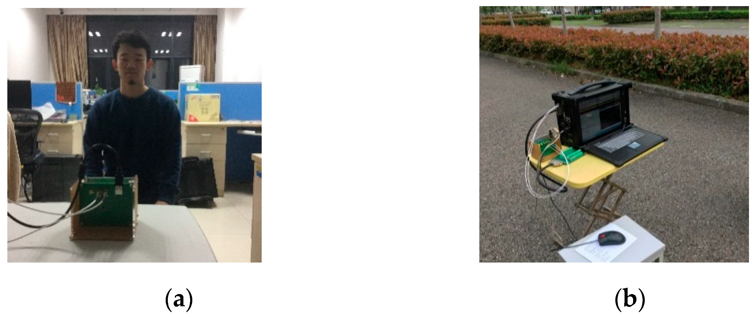
2.1. Experiment Setup

The experiments were performed in the laboratory of the college of Electronic and Information Engineering in Nanjing University of Aeronautics and Astronautics, which is shown in Figure 1a. Figure 1b shows the equipment and system deployment of our experiments. The system, which was employed to collect experimental micro-Doppler signatures of targets, included an IVS-179 radar, an M2i.4912 eight-channel parallel data acquisition card, and an ACME industrial personal portable computer. The IVS-179 radar was connected to the data acquisition card, which in turn was connected to the ACME industrial personal portable computer. The IVS-179 Doppler radar worked at 24 GHz in the continuous wave (CW) mode without modulation and the ACME computer recorded industrial samples at 50 kHz.
We collected data from 10 people, half of whom were women and the other half were men. Each person sat about 1.5 m in front of the radar for about 6 seconds without breathing. For each person, we repeated this procedure 100 times.

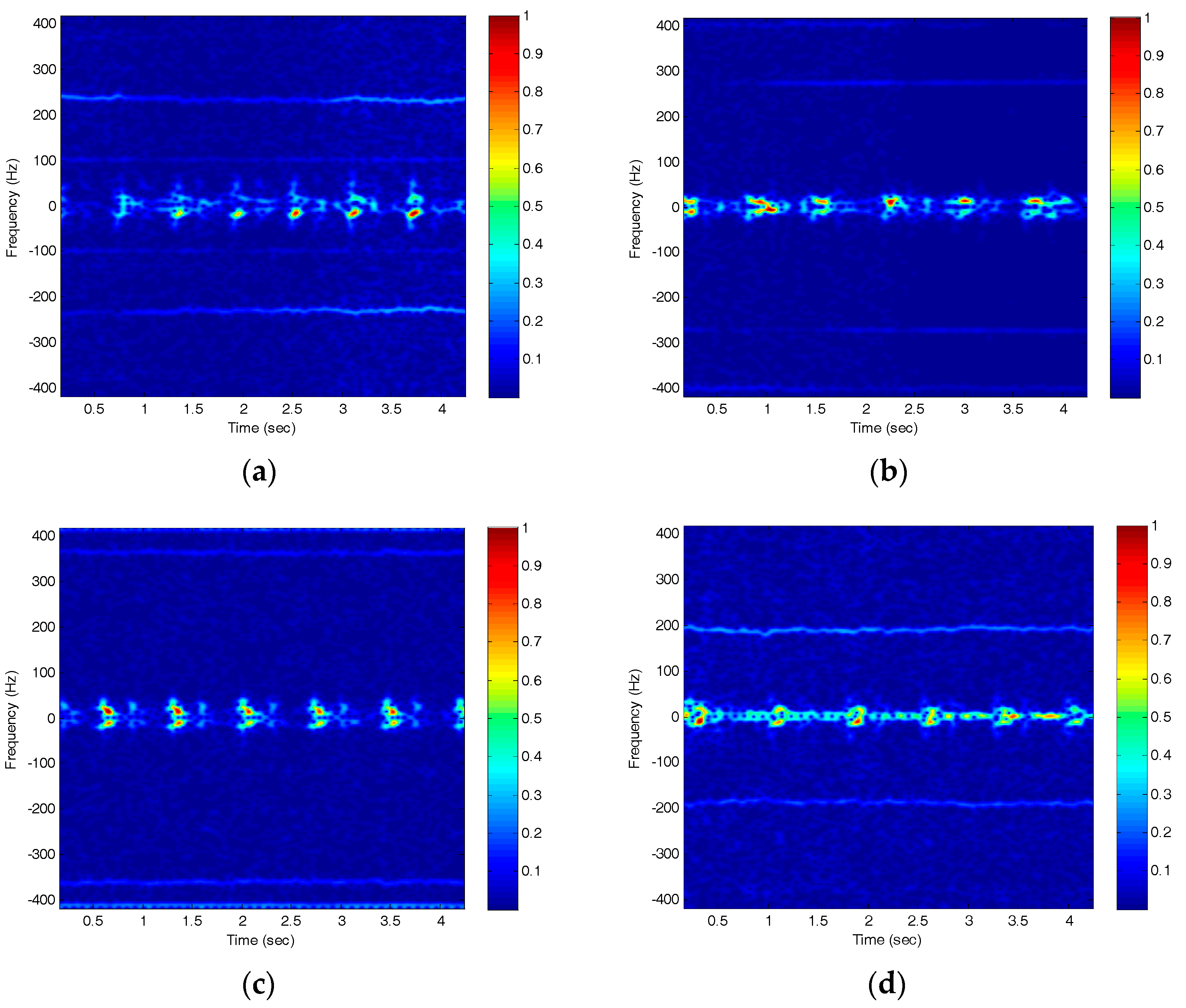
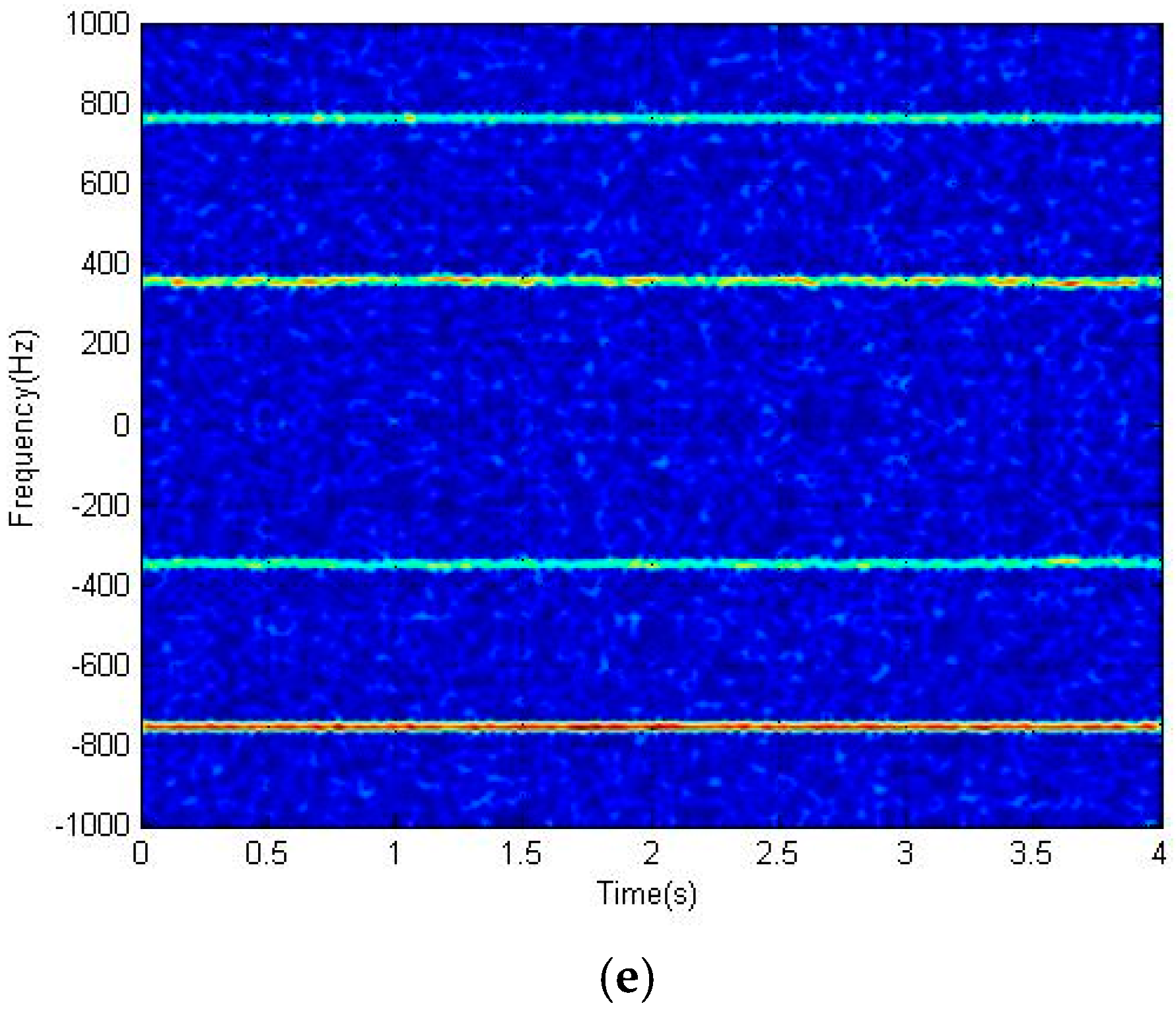
2.2. Micro-Doppler Signatures and Choice of Features

According to the Doppler effect, when a target has motion relative to the wave source, there will be a change in the wavelength of a wave. Meanwhile, if some parts of the target have micro-motion, there will be the micro-Doppler effect, where the additional frequency components in addition to the main Doppler shift can be observed in the joint time–frequency space [13]. Therefore, short-time Fourier transform (STFT) is exploited to characterize micro-Doppler signatures.
Suppose the window function is g ( t ) , which will slide along the time line. The time domain Doppler signal is x ( t ) , and its STFT [14] can be expressed as
F S T F T x ( t , f ) = + x ( u ) g ( u t ) exp ( j 2 π f u ) d u .
In our work, we chose a Gaussian window, so F S T F T x ( t , f ) can be expressed as
F S T F T x ( t , f ) = + x ( u ) exp ( ( ( t u ) 2 σ 2 ) ) exp ( j 2 π f u ) d u ,
In the process, the proper time window size and sliding step are vital in capturing the micro-Doppler feature of a target in the time–frequency domain. After repeated practice, we chose 0.139 s as the time window and set the sliding step size to 1/2000 s. The spectrograms of heartbeats from four different people are shown in Figure 2. It is apparent that the heartbeat for everyone is unique. First, from the graphs, we can see that the heartbeat differs in period (horizontal distance between yellow/red dots) and energy (color of the dots). Additionally, their bandwidth (vertical extension) and shape are different from each other. In order to get sufficient data for the DCNN, we divided the test data into three parts equally. After that, we employed basic image transformation methods to the graphs like translation, rotation, zoom, mirroring, and cropping. These methods are often used to augment the dataset, as the character of the images will not be altered by these transformations, which means the classification results will not be influenced. After these operations, the number of spectrograms for each person was 4000.
For conventional supervised learning methods, we extracted features from the spectrograms. Features adopted in this paper are listed as follows:
(1)
The period of the heartbeat;
(2)
The energy of the heartbeat;
(3)
The bandwidth of the Doppler signal.
The total energy of the radar signal is
E = S B ( t ) S B ( t )
where E represents the energy of the signal and S B represents the radar signal.
We normalize the energy by dividing each signal through its respective energy:
E n o r m = S B ( t ) E
where E n o r m represents normalized energy.

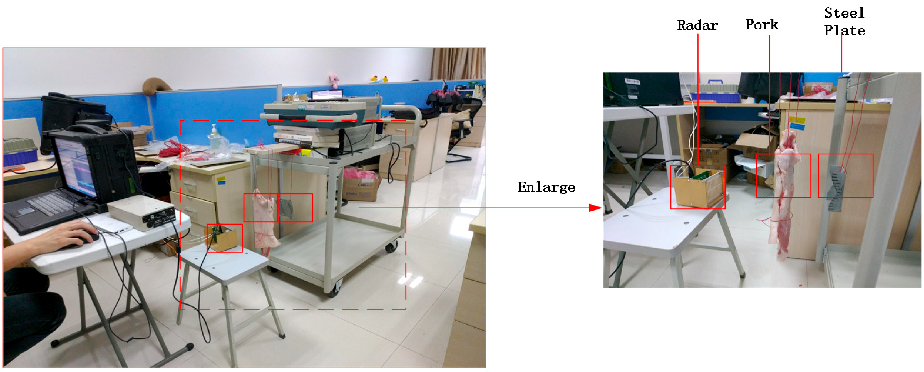
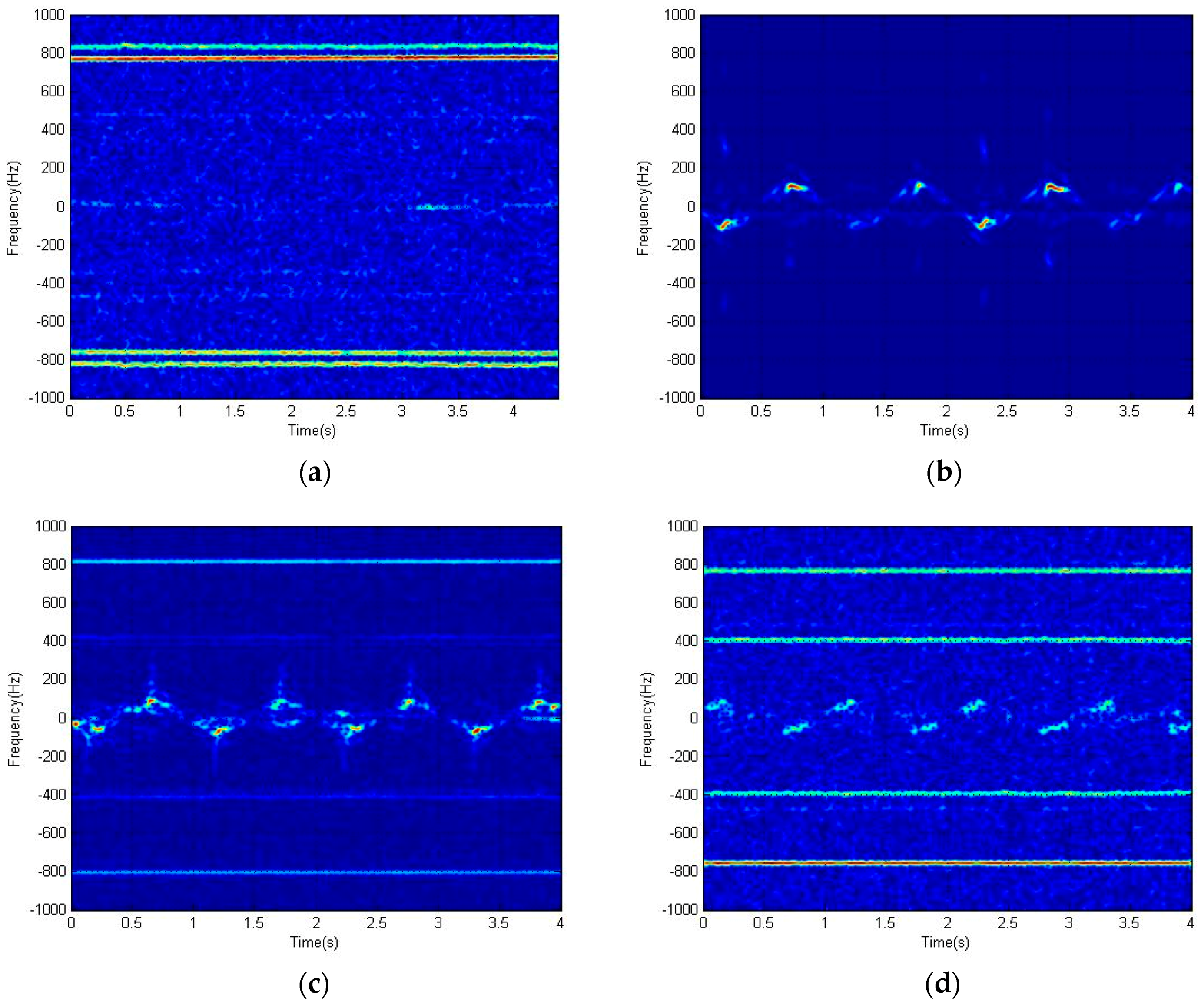
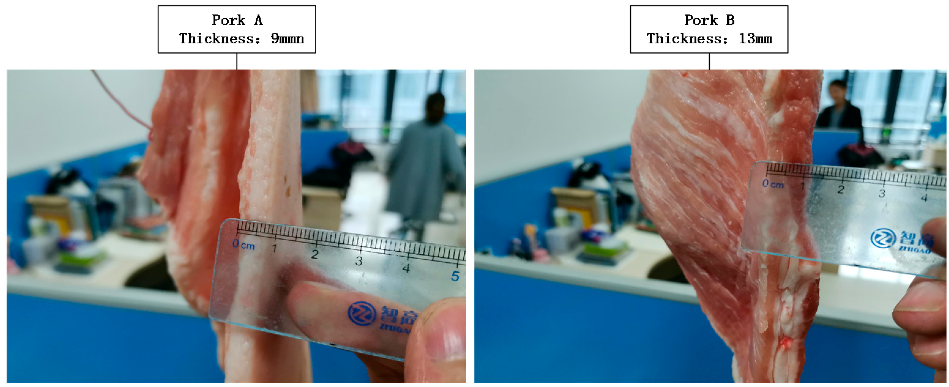
2.3. Experiment on the Penetrability of the Radar

The radar we employed was a 24 GHz radar, with which we did experiments on the radar penetration of skin. The experiment was performed in the laboratory of the college of Electronic and Information Engineering in Nanjing University of Aeronautics and Astronautics, which is shown in Figure 3. During the experiment, a steel plate and pieces of pork were used to simulate a moving target. They moved back and forth as a rope was pulled. We used two pieces of pork to replace human tissue for the experiment (see Figure 4). The thicknesses of the pieces of pork were 9 mm and 13 mm (+/−2 mm measurement error). The pork was placed between the radar and the pendulous steel plate. When there was no pork between the radar and the pendulous steel plate, the radar could receive the reflection from the steel plate, which is shown in Figure 5b. When there was no subject in front of the radar, no micro-Doppler signal could be observed (Figure 5a). When pork A was placed between the radar and pendulous pork B, no micro-Doppler signal could be observed (Figure 5e). Therefore, a steel plate was a valid analogue for a human heart. We performed the experiment with pork A only (Figure 5c), and pork A and B (Figure 5d) between the radar and the pendulous steel plate. We observed that the micro-Doppler effect of the signal was obvious, which indicated that the shielding effect of pork A was weak and most of the signal could penetrate it. If pork A and B were between the radar and the pendulous steel plate, we observed that the micro-Doppler effect was obviously weakened, which indicated that the shielding effect became stronger. In conclusion, with an increase in thickness, less signal can be received by the radar. Considering the thickness of people’s thoraxes, the signal we received was from the heart.

3. Machine Learning

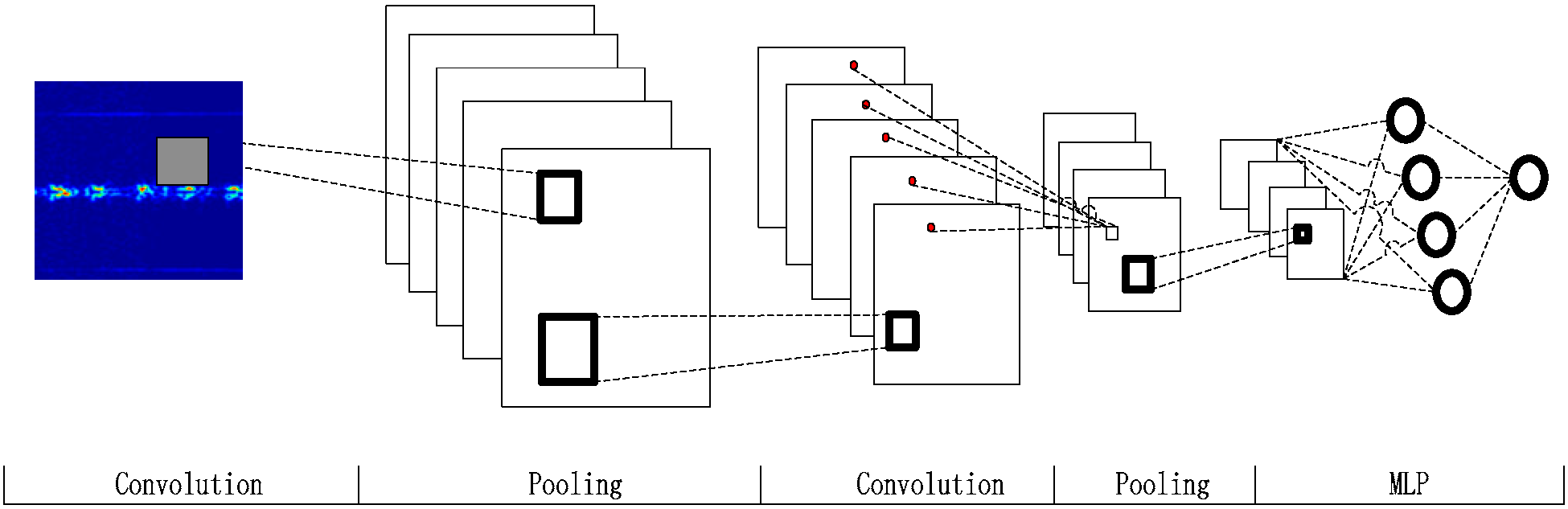
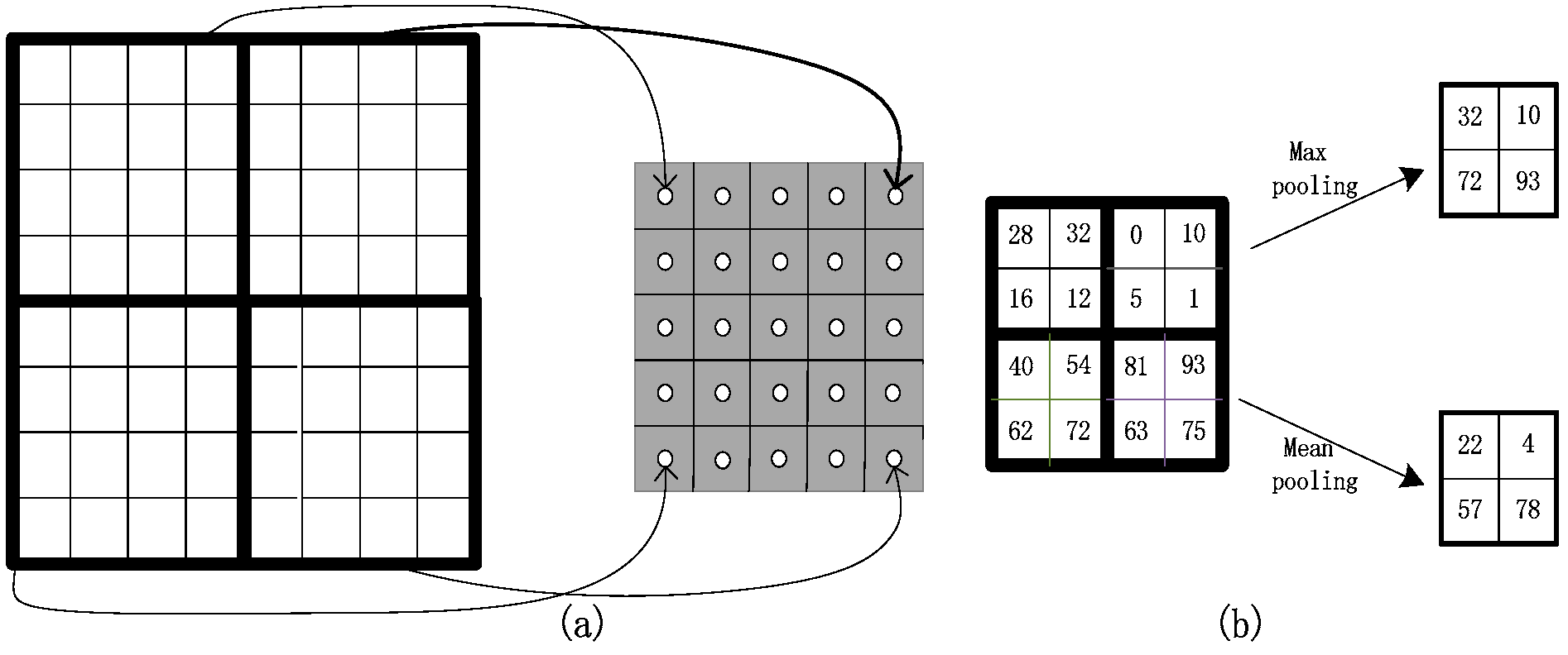
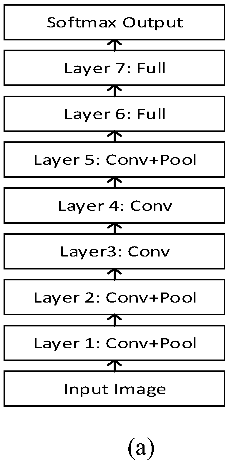
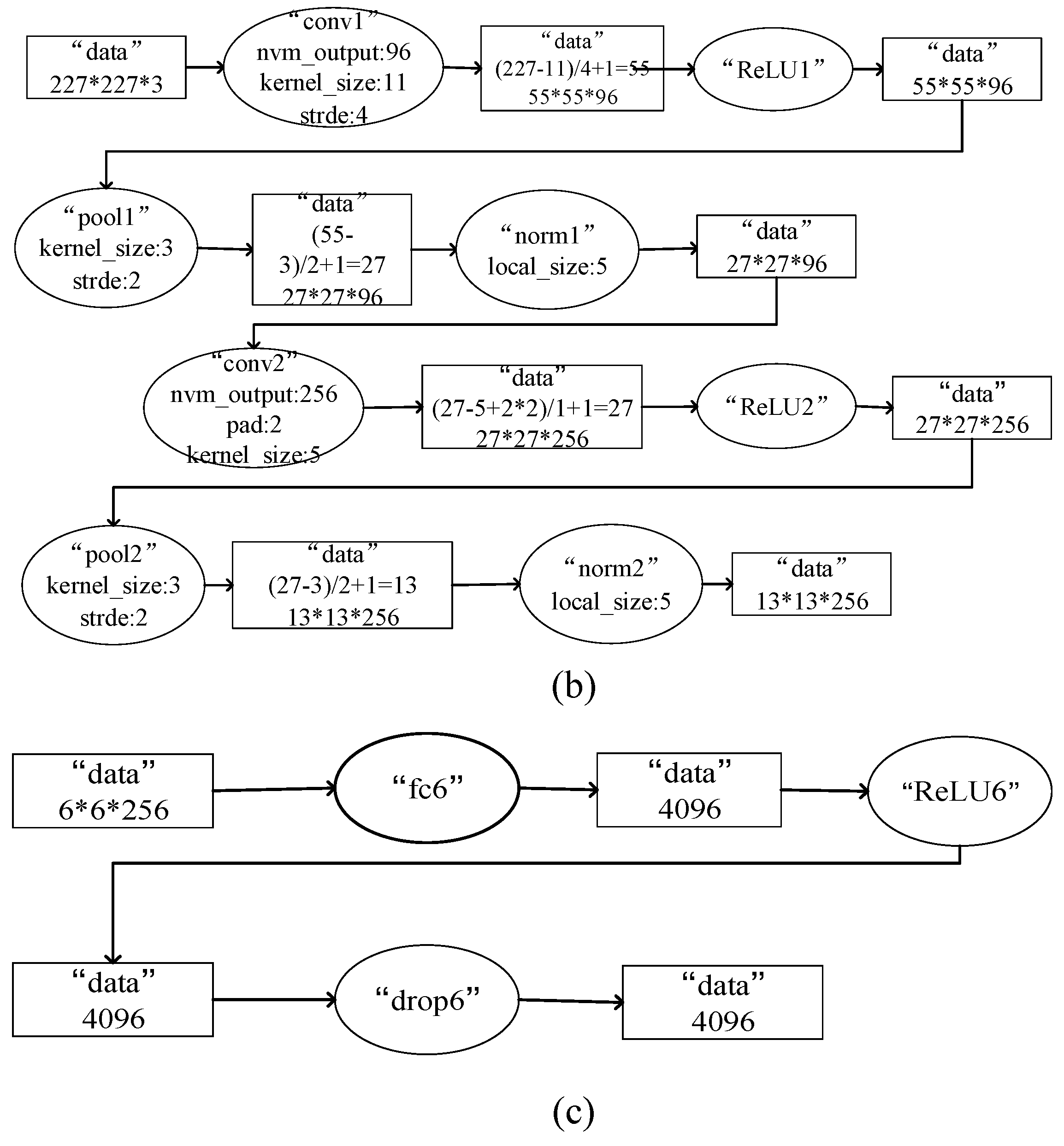
3.1. Deep Convolutional Neural Networks

A deep convolutional neural network (DCNN) is a successful deep learning algorithm that can be employed to classify new samples or intelligently predict possibilities by learning the underlying patterns and characteristics from existing data. In recent years, it has performed well in various fields such as image recognition and speech recognition in numerous researchers’ studies. It is a kind of multilayer supervising learning neural network. The key components of a DCNN are the convolution and pooling operation in the hidden layer, which are used for feature extraction. Multiple convolution filters work in parallel on input data to build the feature maps in the convolutional layer followed by the pooling layer. A simple DCNN architecture with two convolution layers, two pooling layers, and one fully connected layer is shown in Figure 6. Figure 7 shows the schematic diagram of the convolutional and pooling operation. The layers after the feature extraction part of the DCNN are full connection layers, which includes a logistic regression classifier. The input of the full connection is the output of the last pooling layer, and the output of the full connection is the classification results. In our work, we chose softmax regression to classify characteristics. Softmax is developed from logistic regression in order to solve multiclass problems. The function of softmax can be expressed as
h θ ( x ) = [ p ( y ( i ) = 1 | x ( i ) ; θ ) p ( y ( i ) = 2 | x ( i ) ; θ ) p ( y ( i ) = k | x ( i ) ; θ ) ] ,
where p ( y ( i ) = j | x ( i ) ; θ ) represents the probability of the input x ( i ) of the i th sample belonging to category j . θ represents the parameters of the training model. The loss function of the softmax classifier can be expressed as
J ( θ ) = 1 m [ i = 1 m j = 1 k 1 { y i = j } log exp ( θ l T x i ) l = 1 k exp ( θ l T x i ) ] .
In this work, stochastic gradient descent (SGD) was used to minimize the loss function J ( θ ) using the back propagation algorithm until the network converged or reached the maximum iteration. To effectively prevent overfitting, AlexNet employed a dropout operation [11]. The neurons that are in the state of dropout do not participate in the forward propagation or in the back propagation. In this way, the neural network tries a new structure for every input sample, reducing the complex interrelationship of neurons.

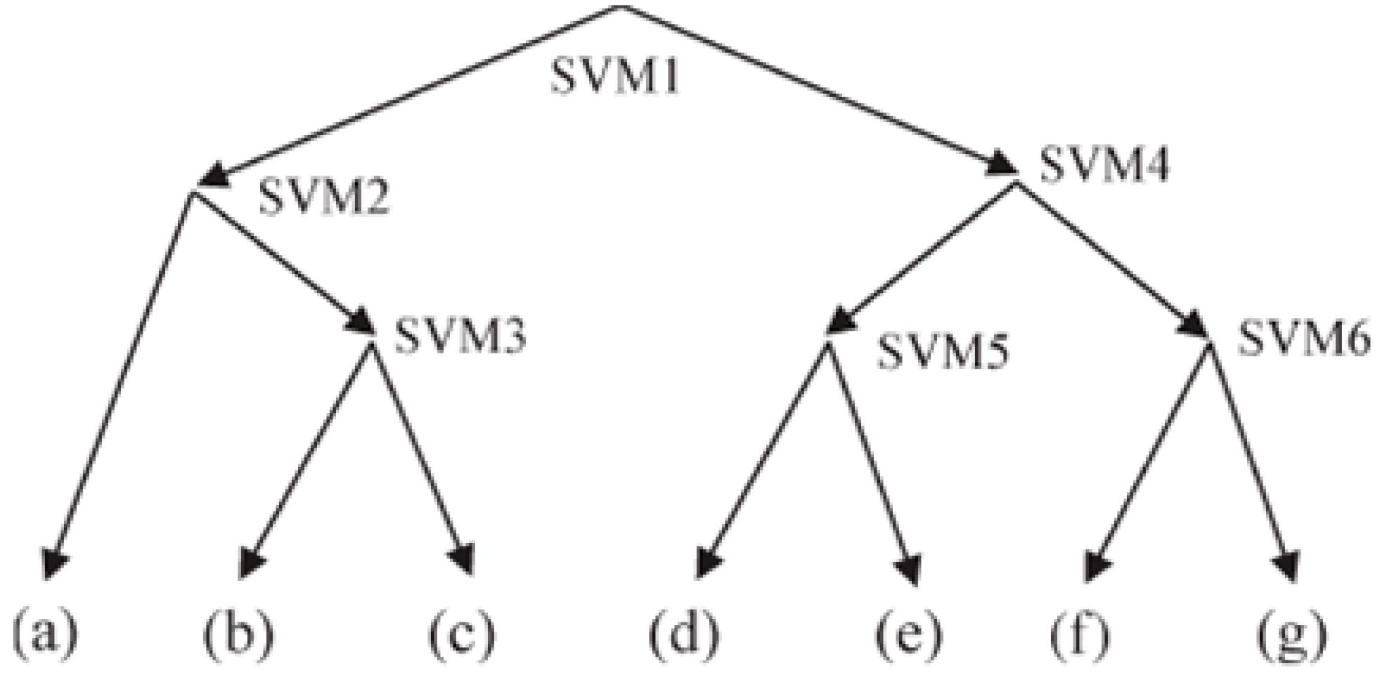
3.2. Support Vector Machine (SVM)

The support vector machine (SVM) based on statistical learning theory (SLT) [15] has performed well in many areas. It is a binary classifier that defines the maximal margin hyperplane in the feature space, followed by the convex quadratic programming optimization algorithm [16]. When classifying targets, the hyperplane is utilized to separate a given set of binary labeled training data. In the conditions where the extracted features cannot be separated linearly, the technique of “kernels” is used to realize a non-linear mapping to a feature space where the linear separation exists.
The j th input point x j = ( x 1 j , , x n j ) , labeled by the variable Y j { 1 , 1 } , is the realization of the random vector X J . ϕ ( x ) is the eigenvector of x after the mapping with the technique of “kernels”. In this paper, we chose Gaussian kernels: K ( x i , x j ) = exp ( x i x j σ 2 ) , where σ is the kernel parameter.
In the feature space, the corresponding decision function is
f ( x ) = w T ϕ ( x ) + b ,
where w is the maximal margin hyperplane:
w = i = 1 m α i y j ϕ ( x i ) ,
while α i are positive real numbers that maximize
i = 1 m α i i j = 1 m α i α j y i y j ( ϕ ( x i ) , ϕ ( x j ) )
subject to
i = 1 m α i y j = 0 ,   α i > 0 .
The decision function can be equivalently expressed as
f ( x ) = i = 1 m α i y i ϕ ( x i ) T ϕ ( x ) + b .
SVM is a two-class classifier. In order to apply it to the multiclass problem like the one at hand, it should be modified into several binary class problems. Several works have been done to handle multiclass problems using SVMs [17,18]. In this paper, we employed one of these methods that combines SVMs with a decision-tree classifier. The configuration of this method is shown in Figure 8. The decision-tree method breaks multiple classes into several distinct binary decision problems using a tree structure. At each nonleaf node of the structure, a binary SVM classifier is used, which is simple and intuitive.
The complexity of SVM is not decided by the number of samples of the training set, but is related to the number of the supported vectors, which indicates that SVM has a simple system structure. Furthermore, it costs little time in the training and testing period, making it popular for pattern recognition, image recognition, and many other fields.

3.3. Naive Bayes (NB)

Naive Bayes (NB), which is based on Bayes’ [19,20] theorem, has the smallest misclassification rate when the conditional independence assumption is valid. Theoretically, the assumption will limit its application, but in fact, not only does the complexity of naive Bayes reduce exponentially, but also considerable robustness and efficiency are shown in many conditions that are opposition to the assumption. Considering its efficient evaluation, high accuracy, and solid theory foundation, it has been successfully applied to data mining tasks including classification, clustering, and the selection of models. Theoretically, the probability model for the Naive Bayes classifier can be expressed as follows.
For a given dataset ( T = { ( x 1 , y 1 ) , ( x 2 , y 2 ) , , ( x N , y N ) } ), the Bayes formula can be expressed as
P ( Y i | X ) = P ( X | Y i ) P ( Y i ) k [ P ( X | Y k ) P ( Y k ) ] .
Naive Bayes learns the joint probability ( P ( X , Y ) ) of input and output based on the conditional independence assumption. On this basis, for a given input ( X ), the method figures out the output ( Y ) with the maximum posterior probability using Bayes’ theorem. Naive Bayes can be equivalently expressed as
y = f ( x ) = arg max c k P ( Y = c k ) j P ( X ( j ) = x ( j ) | Y = c k ) k P ( Y = c k ) j P ( X ( j ) = x ( j ) | Y = c k ) .
When the input is x , the category with the highest conditional probability is chosen as the class to be classified after calculating the conditional probability of all categories. Since the denominator of Formula (13) is the same for all c k , Formula (13) can be simplified as
y = f ( x ) = arg max c k P ( Y = c k ) j P ( X ( j ) = x ( j ) | Y = c k ) .

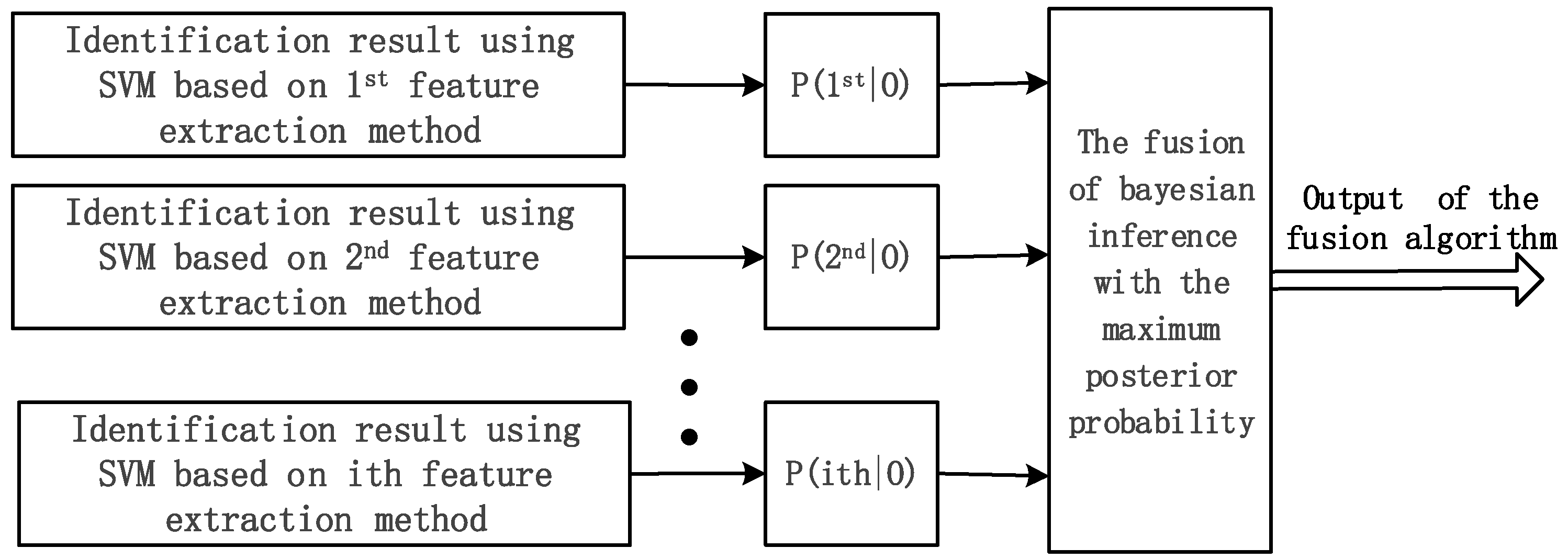
3.4. SVM–Bayes Fusion

To explore whether better results can be achieved by the fusion of different conventional supervised learning methods, a fusion algorithm of SVM and Bayes was employed to process the extracted features. Figure 9 shows the schematic diagram of this fusion algorithm. In the process of Bayesian inference, when there is no empirical data available, the subjective probability can be used to substitute the prior probability as well as the likelihood function of the hypothetical event.
Let us assume that there are m kinds of feature extraction methods, n categories, and let Θ represent the collections of the categories ( Θ = { O 1 , O 2 , , O n , } ). The fusion algorithm is based on maximum a posteriori (MAP). For an unknown sample ( O Θ ), it can be expressed as
P ( O M A P | O 1 , O 2 , , O m ) = max O Θ P ( O | O 1 , O 2 , , O m ) ,
where O i is the decision for an unknown sample of SVM using the i th feature extraction method. O M A P is the decision of the sample based on multi-feature extraction methods. P ( O M A P | O 1 , O 2 , , O m ) is the joint probability density function of SVM based on m kinds of feature extraction methods. Then Formula (15) can be expressed as
O M A P = Δ arg   max O Θ P ( O | O 1 , O 2 , , O m ) .
According to Bayes’ Formula (12), the fusion algorithm can be expressed as
O M A P = Δ arg max O Θ { P ( O 1 , O 2 , , O m | O ) P ( O ) O Θ P ( O 1 , O 2 , , O m | O ) P ( O ) } ,
where P ( O ) is prior probability of O Θ .
The denominator of the equation is the full probability formula. This is not affected by the value of O , so it can be simplified as
O M A P = Δ arg max O Θ { P ( O 1 , O 2 , , O m | O ) P ( O ) } .
Since the feature extraction methods are independent, the equation can be expressed as
O M A P = Δ arg max O Θ { P ( O ) i = 1 m P ( O i | O ) } ,
where P ( O i | O ) is the likelihood function of SVM based on the i th feature extraction method. As the logarithm of this function is monotone increasing, the logarithm on the right side of Formula (19) can simplify the operation without affecting the fusion recognition decision. Then the equation can be expressed as
O M A P = Δ arg max O Θ { ln P ( O ) + i = 1 m ln P ( O i | O ) } .
P ( O ) and P ( O i | O ) need to be confirmed. P ( O ) is prior probability, and in this case, it is assumed that each person has the same probability. The likelihood function P ( O i | O ) means that when the identity of the person is certain, the probability that the person can be correctly identified by SVM. Its value can be approximated by the recognition experiment of training samples.

4. Results and Discussion

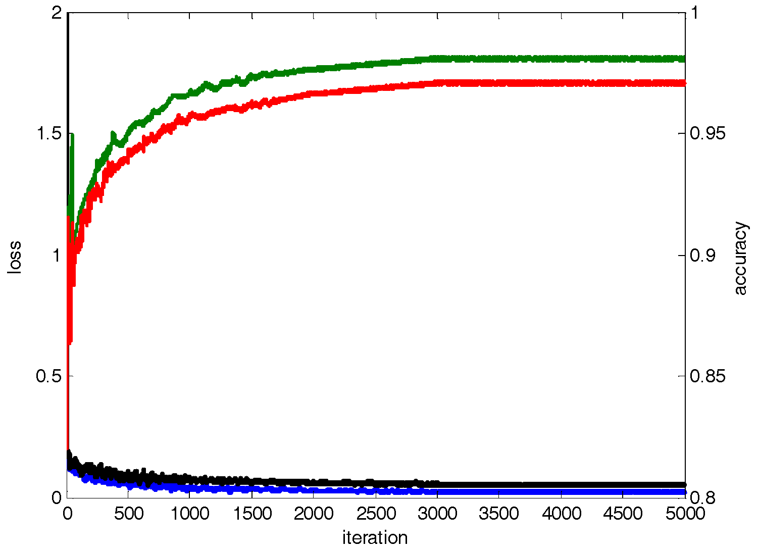
4.1. Based on Deep Learning

We employed the DCNN to the measured, experimental spectrograms directly to classify different humans. Then the human identification problem was transformed into an image recognition problem. For training data, 80% of the spectrograms of each person were used, and the rest were used to test. We employed Caffe [21], i.e., convolutional architecture, for fast feature embedding, which is open-source and speeded up by the NVIDIA Graphics Processing Unit (GPU) and Compute Unified Device Architecture (CUDA) library, as the platform to analyze the spectrograms. The GPU we used is the NVIDIA Quadro M4000.
We adopted AlexNet, in which there were five convolution layers, two fully connected layers with 4096 hidden nodes in the first fully connected layer, and an output layer as shown in Figure 10a. The size of the input pictures of the whole AlexNet must be 256 × 256 , which can be normalized by the tools of Caffe directly. The partial internal structure of the network is shown in Figure 10. Figure 10b shows the first two convolutional layers and pooling layers, while Figure 10c shows the first full connection layer. In our work, rectified linear units (ReLU) were used as the activation function and were followed by max pooling in each layer. We fine-tuned the parameters of the network according to our experiments, and this was recorded in the configuration file of Caffe. The data of the learning rate was adjusted to 0.001 because when the learning rate was larger, the loss would not converge, and when the learning rate was smaller, the process was time-consuming. In our experiments, we allowed up to 5000 iterations for stable results. The learning rate was reduced to 0.001 × 0.9 ^ ( f l o o r ( 5000 / 2000 ) ) after every 2000th iteration, since we employed the gradient descent method to solve the optimization problem. The weight decay was changed to 0.001 to prevent overfitting. The definition of the network for training and validation as well as the parameters for every layer were recorded in a particular file. In this file, the spectrograms were resized to 227 × 227 , since the size of the input spectrograms of the first convolution layer must be 227 × 227 . The batch sizes in the “train” part and “test” part were adjusted to 48 and 24 respectively. Batch size represents the number of samples taken in each iteration. The average of the gradient of those samples was used to update the parameters of the network. The batch size determines the direction of gradient descent and the effect and rate of convergence, as well as memory utilization. In the fully connected layer, we adapted the learning rate of bias to 15 and the learning rate of weight to 20 to speed up the learning rate in these layers. After 5000 iterations, our own network was generated and stored all relevant model parameters, like weight, that were suitable for our own spectrograms.
We assessed the performance of our network under the scenario where we recognized one person from a group. We randomly selected 100 spectrograms for each person from the test data to verify the stability of our own network, and calculated the time it took to classify one person. The whole process was repeated 100 times. The variance of the 100 times was 0.007, which means that the repeated 100 times varied slightly with each other, and our network was very stable.
Figure 11 shows the accuracy as well as the loss (see Equation (6)) of the training and testing process for four humans. The loss shown is the value of the loss function in Formula (6). It can be observed that as the iteration grew, the accuracy and loss became stable, and the loss tended to 0, which means that the process was not overfit. Figure 12 shows the confusion matrices of a random time for the identification results of the DCNN. Since the results of the repeated 100 times varied slightly, the result of one time could represent the accuracy to some extent. From the figures, we can see that as the number of the group became larger, the accuracy of the human identification declined. However, the average accuracy of the group below 10 was higher than 80%, which can be compared to the identification methods based on optical systems [22].

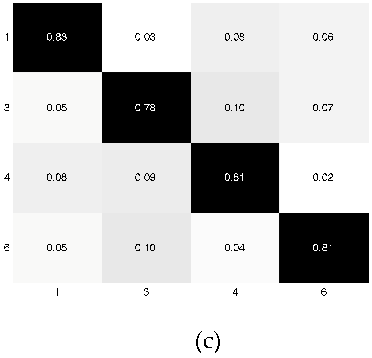
4.2. Based on Conventional Supervised Learning Algorithms

SVM and NB were applied to the extracted features (heartbeat period, energy, and bandwidth) for the human identification problem. The amount of data required in this part was relatively small compared with that utilized in the DCNN, which is one of the advantages of conventional supervised learning methods. In this paper, the fusion of two conventional supervised learning methods, SVM and Bayes, was employed with the aim of getting a better result. Figure 13 shows the confusion matrices of SVM–Bayes, SVM, and NB respectively. It can be observed that SVM–Bayes has the highest accuracy—91.25% among the three algorithms, followed by SVM, and the lowest accuracy is NB. The average accuracy of SVM is higher than that of NB, which is 88.75% and 80.75% respectively. Though the results for each of them are satisfying, they all have high misclassification in identifying some people compared with the DCNN.

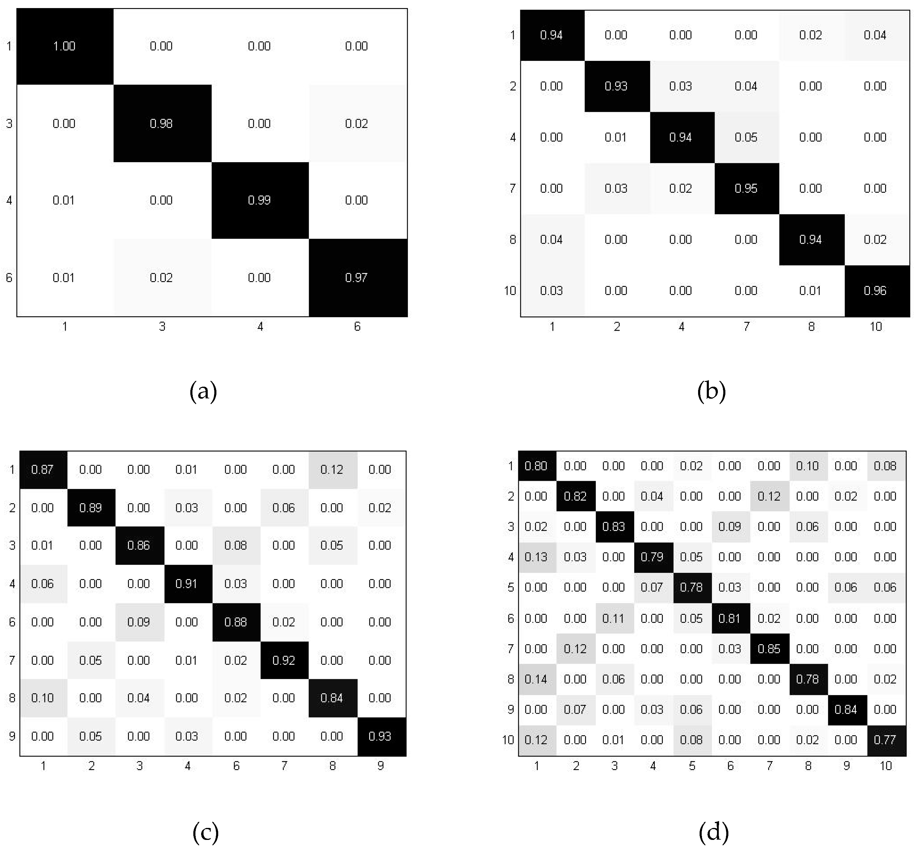
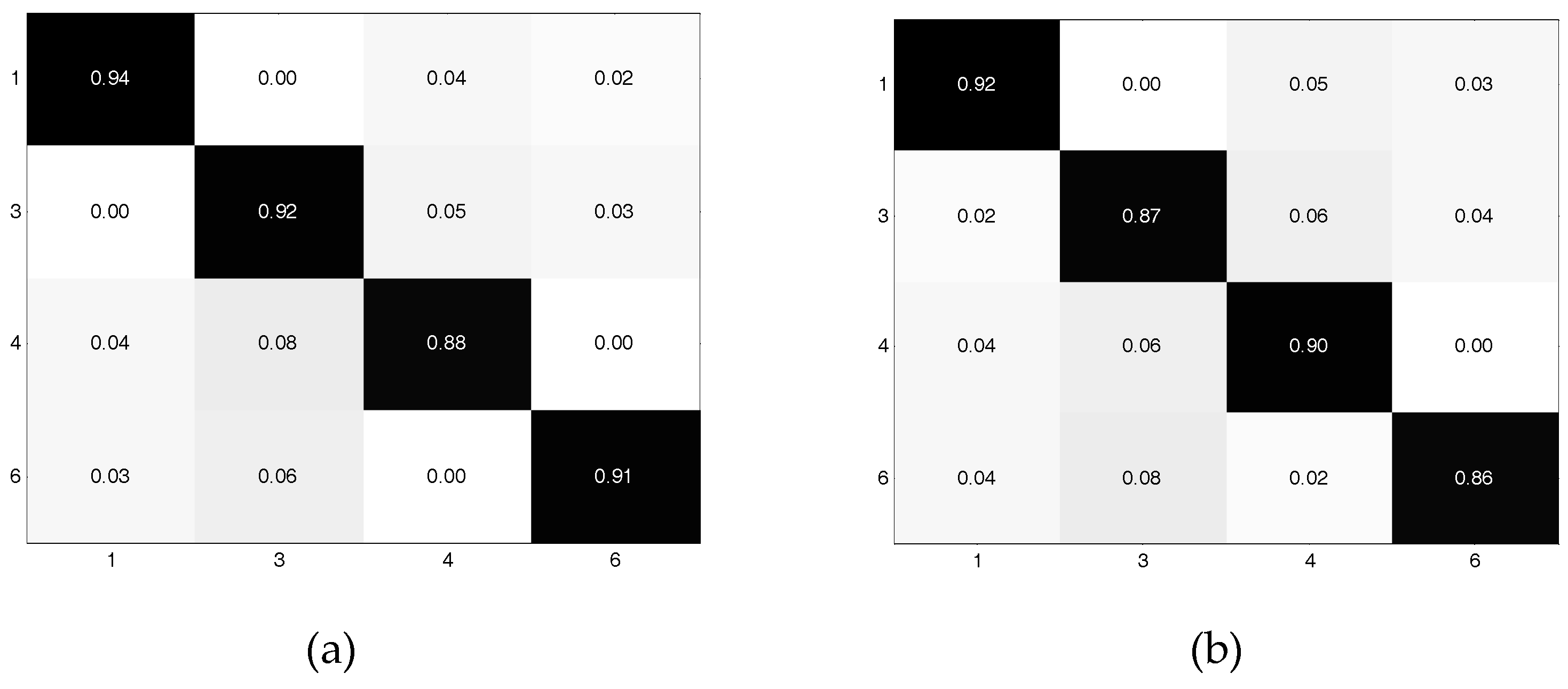
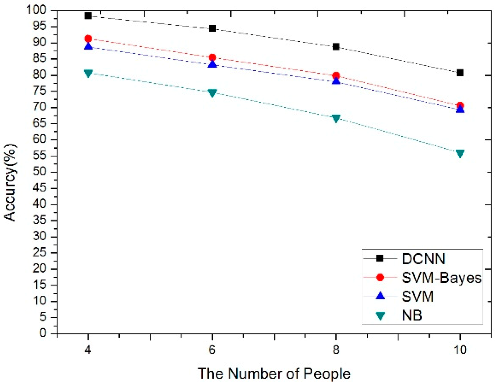
4.3. The Impact of Noise and Human Number for the Four Algorithms

To study the robustness of our classification algorithms, we challenged each algorithm by adding noise to the respective input. We added different levels ( S N R = 29   dB ~ 30   dB ,   20   dB ~ 21   dB , 10   dB ~ 11   dB , 0   dB ~ 1   dB ) of random noise to the raw radar signal. For example, we added random noise ( S N R = 0   dB ~ 1   dB ) to the raw signals that we collected in Section 2. After that, we randomly chose 100 spectrograms of each target at each noise grade to test the noise immunity of the algorithm. For each noise grade, the whole process was repeated 100 times, and the average accuracy was taken as the final result. As for detecting the anti-noise performance of SVM, NB, and the SVM–Bayes fusion algorithm, we also added different grades ( S N R = 29   dB ~ 30   dB ,   20   dB ~ 21   dB , 10   dB ~ 11   dB , 0   dB ~ 1   dB ) of random noise to the signals that we collected in Section 2, and we followed this with feature extraction. Figure 14 compares the accuracy of the four different algorithms with different levels of noise. From this figure, we can observe that the DCNN had the highest accuracy of human identification at all noise levels, followed by SVM–NB, then SVM, and NB had the lowest accuracy. Additionally, it can be observed that the noise resistance of SVM–Bayes and SVM were very similar, while the DCNN had the best noise resistance and NB had the worst.
Figure 15 shows the impact of the number of individuals in each test run of the four classification algorithms on the accuracy of correct identification. As can be observed, the accuracy of recognition decreased as the number of humans increased. Additionally, the DCNN had the best performance of the four algorithms. The accuracy of the SVM–Bayes fusion algorithm was a little bit higher than that of SVM, but as the number of people increased, the accuracy of the SVM–Bayes fusion algorithm dropped more quickly than SVM.
Table 1 shows the average accuracy of identifying four people with the four methods. It can be observed that the DCNN performed better than the conventional supervised learning methods and the SVM–Bayes fusion method, while NB had the lowest accuracy. Additionally, the fusion algorithm of SVM and Bayes performed better than the two separate conventional supervised learning methods, which means that the fusion algorithm can be further studied. Training time is the time it takes to train the network to the condition of four people, while the identification time means the time it takes to identify one spectrogram or a set of features using the four methods. From Table 1, it can be observed that it took more time to train the DCNN, while the identification time of the four methods was similar.

4.4. Comparison with Other Techniques

In this subsection, we mainly compare results of our method to other methods. Considering that the published papers usually present relatively great results, we have chosen to compare our results with theirs directly. Robinette proposed an approach to identify humans based on extracted gait features using images [22]. The maximum group size of this approach was 11 and its accuracy was 84%, which is close to our results. In [23], WIFI signal was employed to identify different persons for the first time. The maximum group size of this approach was 6, and the average accuracy was 93% for a group of 2 people and 77% for a group of 6 people, which shows that our approach is better both in the number of subjects and the accuracy of identification. Structural vibration induced by footstep was employed for human identification with a maximum group size of 5 [24]. The accuracy for a group of 5 people was 70%, which is less than our method. After these comparisons, we can see that our results are better or no lower than others.

5. Conclusions

In this paper, we realized human identification based on a heartbeat signal from a radar using a DCNN, SVM, NB and the SVM–Bayes fusion algorithm. For the DCNN, accuracy could reach over 80% when the number of the people was below 10, indicating that humans can be identified successfully by the DCNN, while SVM, NB and SVM–Bayes could reach 88.75%, 80.75%, and 91.25%, respectively, for four people. Additionally, the DCNN had excellent performance when the noise and the number of people increased. By contrast, the performances of the conventional supervised methods were far from satisfactory in both aspects. We believe that it shows the potential of DCNNs for human identification problems based on the heartbeat signal from radar micro-Doppler signatures. Compared with conventional supervised methods, the amount of data that a DCNN needs is relatively large. In the future, further research will be done for the purpose of improving identification performance. First, the condition we considered in the experiments, where humans sat just 1.5 m in front of the radar, is simple compared with realistic conditions. In the future, we will do further research on data acquisition at long range or non-line of sight (NLOS) scenarios. Second, our experiments only comprised ten people. To apply our system to the real world, we need to include more people. In addition, the optimization for the frame of the network also lies in our future research plan.

Author Contributions

Conceptualization, P.C. and W.X.; methodology, validation, formal analysis, data curation, original draft preparation and writing, P.C.; review, editing, and funding acquisition, W.X.; data curation, Y.L.

Funding

This research was funded by the National Natural Science Foundation of China (Grant no. 6150010825), the Fundamental Research Funds for the Central Universities (Grant no. NS2016040), the Fundamental Research Funds for the Central Universities (Grant no. NJ20150020), and the China Scholarship Council (Grant no. 201606835062).

Acknowledgments

The work was supported by the National Natural Science Foundation of China (Grant no. 6150010825), the Fundamental Research Funds for the Central Universities (Grant no. NS2016040), the Fundamental Research Funds for the Central Universities (Grant no. NJ20150020), and the China Scholarship Council (Grant no. 201606835062).

Conflicts of Interest

The authors declare no conflict of interest.

References

  1. Molchanov, P.; Astola, J.; Egiazarian, K. Classification of ground moving radar targets by using joint time-frequency analysis. In Proceedings of the IEEE Radar Conference, Atlanta, GA, USA, 7–11 May 2012; pp. 366–371. [Google Scholar]
  2. Villeval, S.; Bilik, I.; Gürbüz, S.Z. Application of a 24 GHz FMCW automotive radar for urban target classification. In Proceedings of the IEEE Radar Conference, Cincinnati, OH, USA, 19–23 May 2014; pp. 1237–1240. [Google Scholar]
  3. Tahmoush, D.; Silvious, J.; Burke, E. A radar unattended ground sensor with micro-Doppler capabilities for false alarm reduction. In Proceedings of the Conference on Unmanned/Unattended Sensors and Sensor Networks VII, Toulouse, France, 20–23 September 2010; pp. 20–22. [Google Scholar]
  4. Robinette, C.D.; Silverman, C.; Jablon, S. Effects upon health of occupational exposure to microwave radiation (radar). Am. J. Epidemiol. 1980, 112, 39–53. [Google Scholar] [CrossRef]
  5. Chen, V.C. The Micro-Doppler Effect in Radar; Artech House: Norwood, MA, USA, 2011. [Google Scholar]
  6. Chen, V.C.; Tahmoush, D.; Miceli, W.J. Radar Micro-Doppler Signatures: Processing and Applications; Institution of Engineering and Technology: Stevenage, UK, 2014. [Google Scholar]
  7. Stankovic, L.; Stankovic, S.; Orovic, I. Time Frequency Analysis of Micro-Doppler Signals Based on Compressive Sensing. In Compressive Sensing for Urban Radar; CRC Press: Boca Raton, FL, USA, 2014; pp. 283–326. [Google Scholar]
  8. Zhao, M.; Adib, F.; Katabi, D. Emotion Recognition using Wireless Signals. In Proceedings of the 22nd Annual International Conference on Mobile Computing and Networking, New York, NY, USA, 3–7 October 2016; pp. 95–108. [Google Scholar]
  9. Lin, F.; Song, C.; Zhuang, Y.; Xu, W.; Li, C.; Ren, K. Cardiac Scan: A Non-Contact and Continuous Heart-Based User Authentication System. In Proceedings of the 23rd Annual International Conference on Mobile Computing and Networking, Snowbird, UT, USA, 16–20 October 2017; pp. 315–328. [Google Scholar]
  10. Hinton, G.; Deng, L.; Dong, Y. Deep neural networks for acoustic modeling in speech recognition: The shared views of four research groups. IEEE Signal Process. Mag. 2012, 29, 82–97. [Google Scholar] [CrossRef]
  11. Krizhevsky, A.; Sutskever, I.; Hinton, G. ImageNet classification with deep convolutional neural networks. In Proceedings of the International Conference on Neural Information Processing Systems, Lake Tahoe, NV, USA, 3–6 December 2012; Volume 25, pp. 1097–1105. [Google Scholar]
  12. Huang, R.; Xie, X.; Feng, Z.; Lai, J. Face recognition by landmark pooling-based CNN with concentrate loss. In Proceedings of the IEEE International Conference on Image Processing (ICIP), Beijing, China, 17–20 September 2017; pp. 1582–1586. [Google Scholar]
  13. Javier, R.J.; Kim, Y. Application of linear predictive coding for human activity classification based on micro-Doppler signatures. IEEE Geosci. Remote Sens. Lett. 2013, 11, 781–785. [Google Scholar] [CrossRef]
  14. Chen, V.; Ling, H. Time-Frequency Transforms for Radar Imaging and Signal Analysis; Artech House: Norwood, MA, USA, 2002. [Google Scholar]
  15. Cherkassky, V.; Mulier, F. Statistical Learning Theory. In Learning from Data: Concepts, Theory, and Methods; Wiley-IEEE Press: Hoboken, NJ, USA, 2007; pp. 99–150. [Google Scholar]
  16. Furey, T.S.; Cristianini, N.; Duffy, N.; Bednarski, D.W.; Schummer, M.; Haussler, D. Support vector machine classification and validation of cancer tissue samples using microarray expression data. Bioinformatics 2000, 16, 906–914. [Google Scholar] [CrossRef] [PubMed]
  17. Fumitake, T.; Shigeo, A. Decision-tree-based multi-class support vector machines. Proc. IEEE ICONIP 2002, 3, 1418–1422. [Google Scholar]
  18. Hsu, C.; Lin, C. A comparison of methods for multiclass support vector machines. IEEE Trans. Neural Netw. Mar. 2002, 13, 415–425. [Google Scholar]
  19. Kim, C.J.; Hwang, K.B. Naive Bayes classifier learning with feature selection for spam detection in social bookmarking. In Machine Learning and Principles and Practice of Knowledge Discovery in Databases (ECML/PKDD); Springer Verlag: Antwerp, Belgium, 2008. [Google Scholar]
  20. Pop, I. An approach of the Naive Bayes classifier for the document classification. Gen. Math. 2006, 14, 135–138. [Google Scholar]
  21. Jia, Y.; Shelhamer, E.; Donahue, J. Caffe: Convolutional architecture for fast feature embed-ding. In Proceedings of the 22nd ACM International Conference on Multimedia, Orlando, FL, USA, 3–7 November 2014; pp. 675–678. [Google Scholar]
  22. Ng, H.; Tong, H.L.; Tan, W.H.; Yap, T.T.; Chong, P.F.; Abdullah, J. Human identification based on extracted gait features. Int. J. New Comput. Archit. Their Appl. IJNCAA 2011, 1, 358–370. [Google Scholar]
  23. Zhang, J.; Bo, W. WiFi-ID: Human Identification using WiFi signal. In Proceedings of the IEEE International Conference on Distributed Computing in Sensor Systems, Washington, DC, USA, 26–28 May 2016; pp. 75–82. [Google Scholar]
  24. Pan, S.; Wang, N.; Qian, Y.; Velibeyoglu, I.; Noh, H.Y.; Zhang, P. Indoor Person Identification through Footstep Induced. In Proceedings of the International Workshop on Mobile Computing Systems & Applications, Santa Fe, NM, USA, 12–13 February 2015; pp. 81–86. [Google Scholar]
Figure 1. Data collection setup and experiment scenario. (a) Experiment scenario; (b) The equipment and system deployment of our experiments.
Remotesensing 11 01220 g001
Figure 2. Time–frequency graphs for four different people. (a) Time–frequency graph for person 1; (b) Time–frequency graph for person 2; (c) Time–frequency graph for person 3; (d) Time–frequency graph for person 4.
Remotesensing 11 01220 g002
Figure 3. Setup of the experiment on the penetrability of the radar.
Remotesensing 11 01220 g003
Figure 4. The pork we employed in the experiment.
Remotesensing 11 01220 g004
Figure 5. Time–frequency graphs for different conditions. (a) No subjects in front of the radar; (b) Only a steel plate in front of the radar; (c) Pork A between the radar and steel plate; (d) Pork A and B between the radar and steel plate; (e) Pork A between the radar and pork B.
Remotesensing 11 01220 g005aRemotesensing 11 01220 g005b
Figure 6. A simple deep convolutional neural network (DCNN) architecture.
Remotesensing 11 01220 g006
Figure 7. (a) Process of applying a 4 × 4 convolution filter to the input data to generate the output (in gray). (b) Examples of 2 × 2 pooling (max or mean pooling).
Remotesensing 11 01220 g007
Figure 8. Decision-tree based support vector machine (SVM) classifier.
Remotesensing 11 01220 g008
Figure 9. The framework of the SVM–Bayes fusion algorithm.
Remotesensing 11 01220 g009
Figure 10. (a) The structure diagram of AlexNet, (b) the first two convolution layers and pooling layers, and (c) the first full connection layer.
Remotesensing 11 01220 g010aRemotesensing 11 01220 g010b
Figure 11. The accuracy and loss of the classification process for four humans.
Remotesensing 11 01220 g011
Figure 12. The confusion matrices for the DCNN. (a) is four people, (b) is six people, (c) is eight people, and (d) is 10 people. The x and y axes indicate the serial number of the subjects.
Remotesensing 11 01220 g012
Figure 13. (a) Confusion matrix for SVM–Bayes fusion, (b) confusion matrix for SVM, (c) confusion matrix for naive Bayes (NB). The x and y axes indicate the serial number of the subjects.
Remotesensing 11 01220 g013aRemotesensing 11 01220 g013b
Figure 14. The impact of noise on the four classification algorithms.
Remotesensing 11 01220 g014
Figure 15. The impact of number of humans on the four classification algorithms.
Remotesensing 11 01220 g015
Table 1. Comparison of the results of DCNN, SVM–Bayes, SVM and NB.
MethodAccuracyTraining TimeIdentification Time
DCNN98.5%12 min1.539 s
SVM–Bayes91.25%4.267 s0.771 s
SVM88.75%1.982 s0.643 s
NB80.75%1.674 s0.558 s

