Optimal Strategy of a GPS Position Time Series Analysis for Post-Glacial Rebound Investigation in Europe


Abstract
1. Introduction
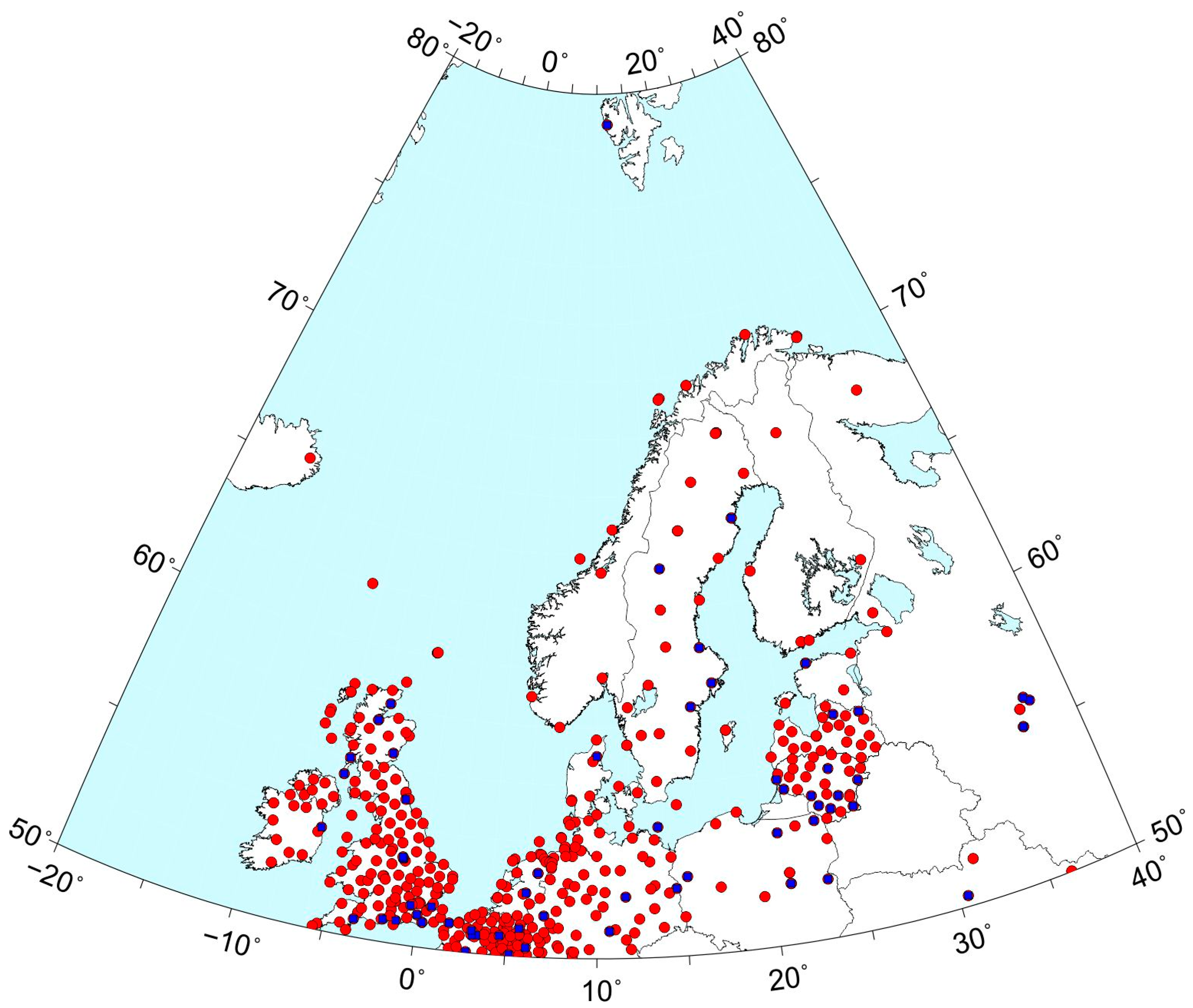
2. Dataset
3. Methods
4. Results
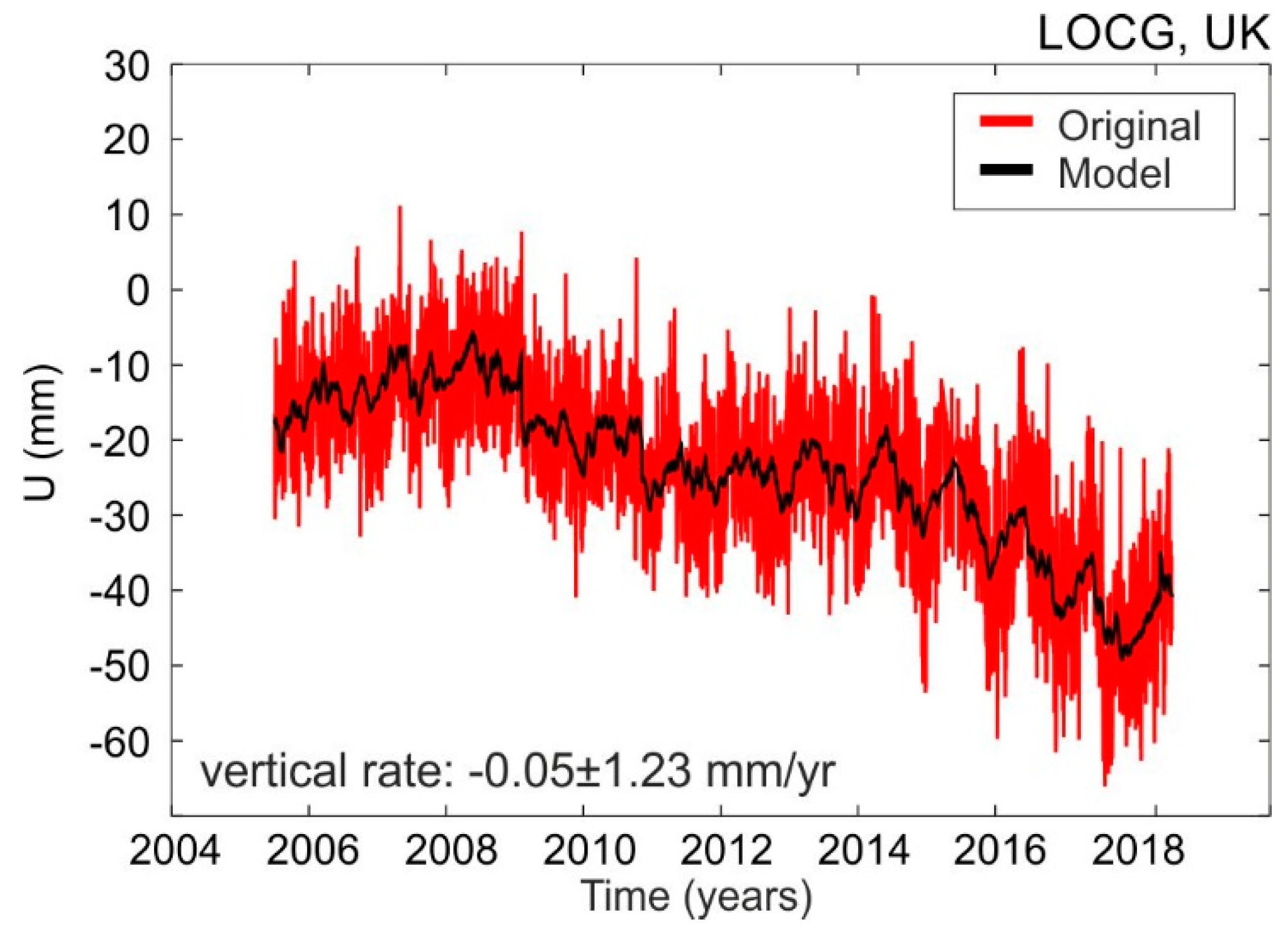
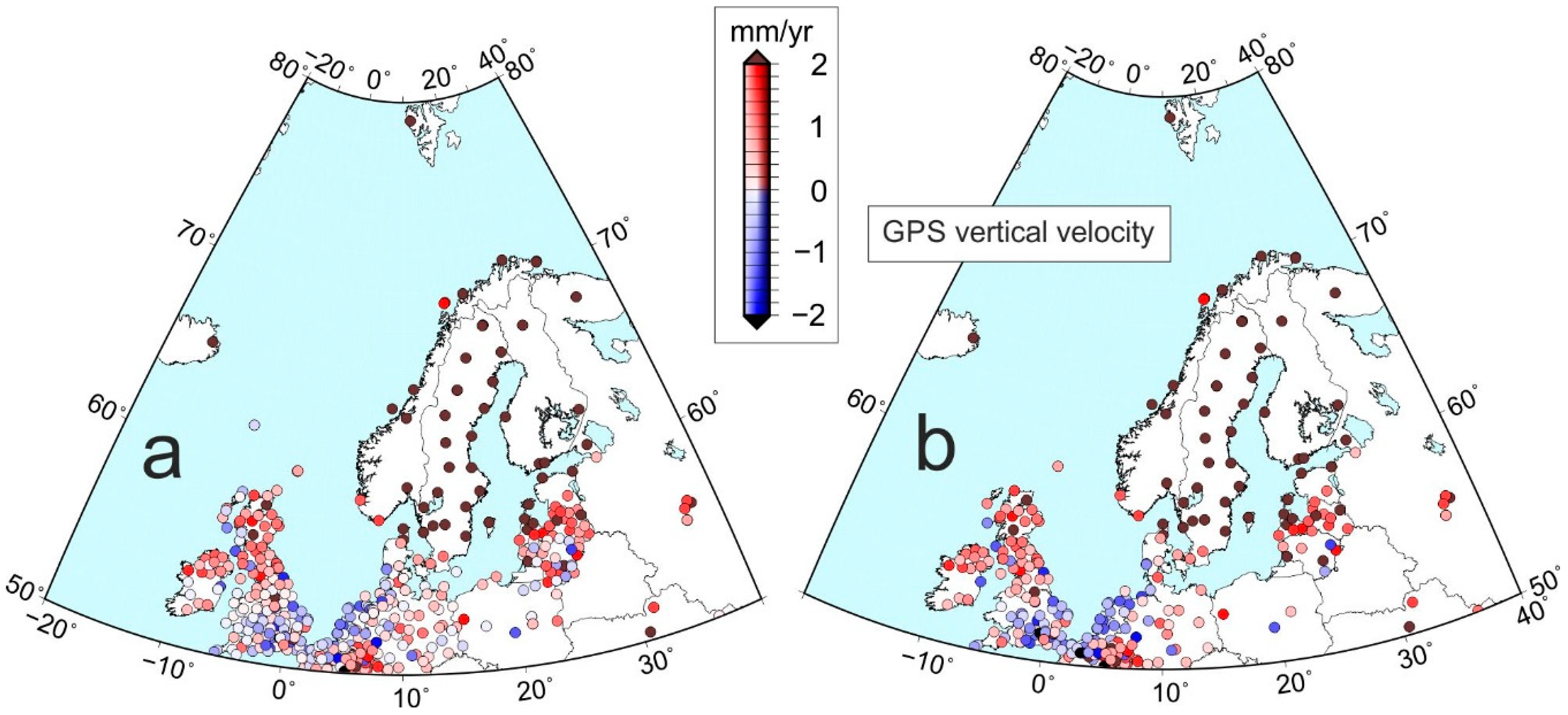
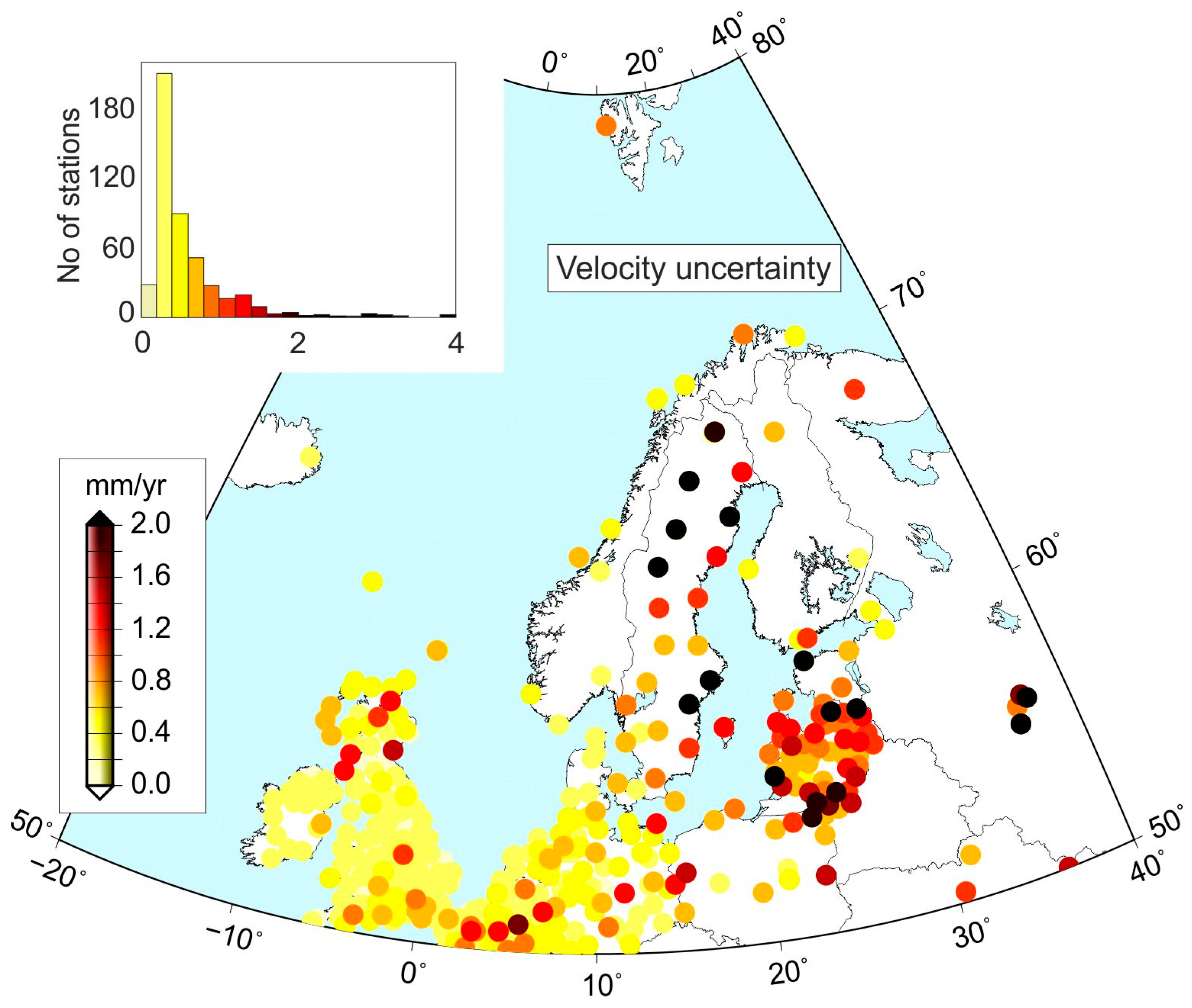
4.1. GPS-Derived Vertical Velocities
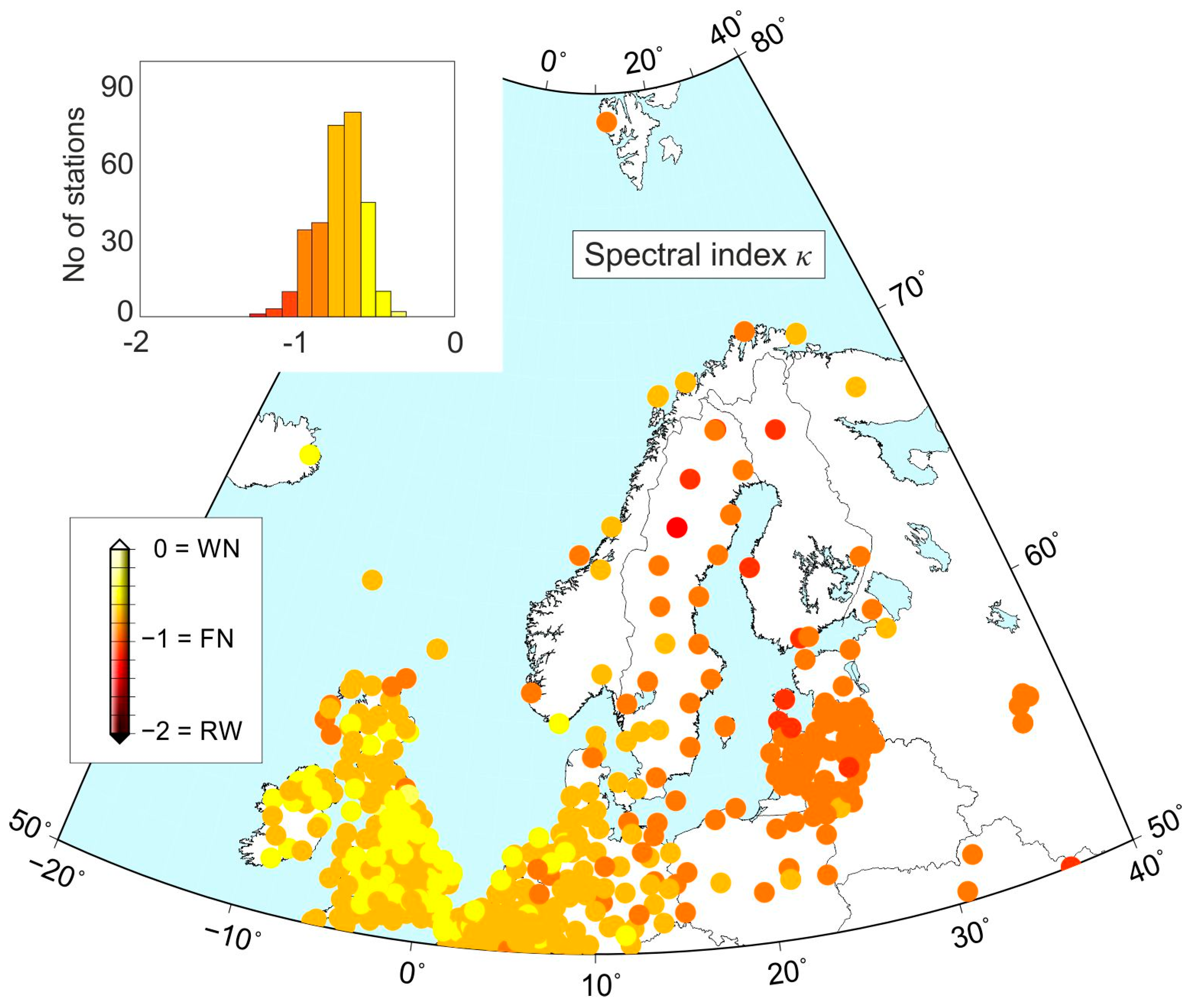
4.2. Noise Analysis
4.3. Statistical Significance of Vertical Rates
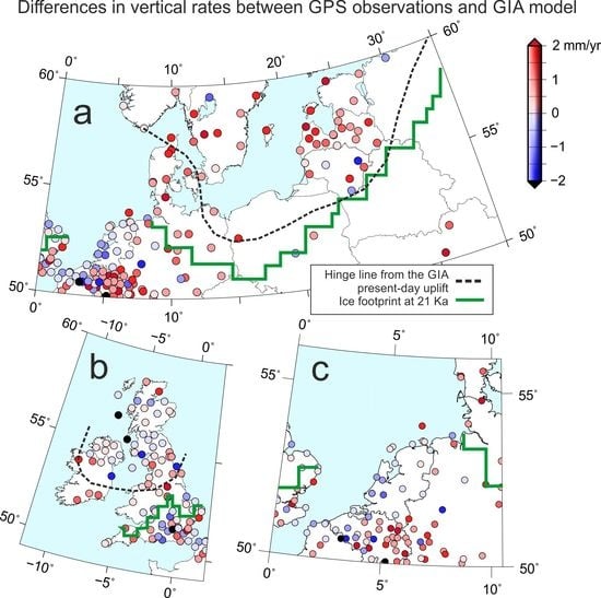
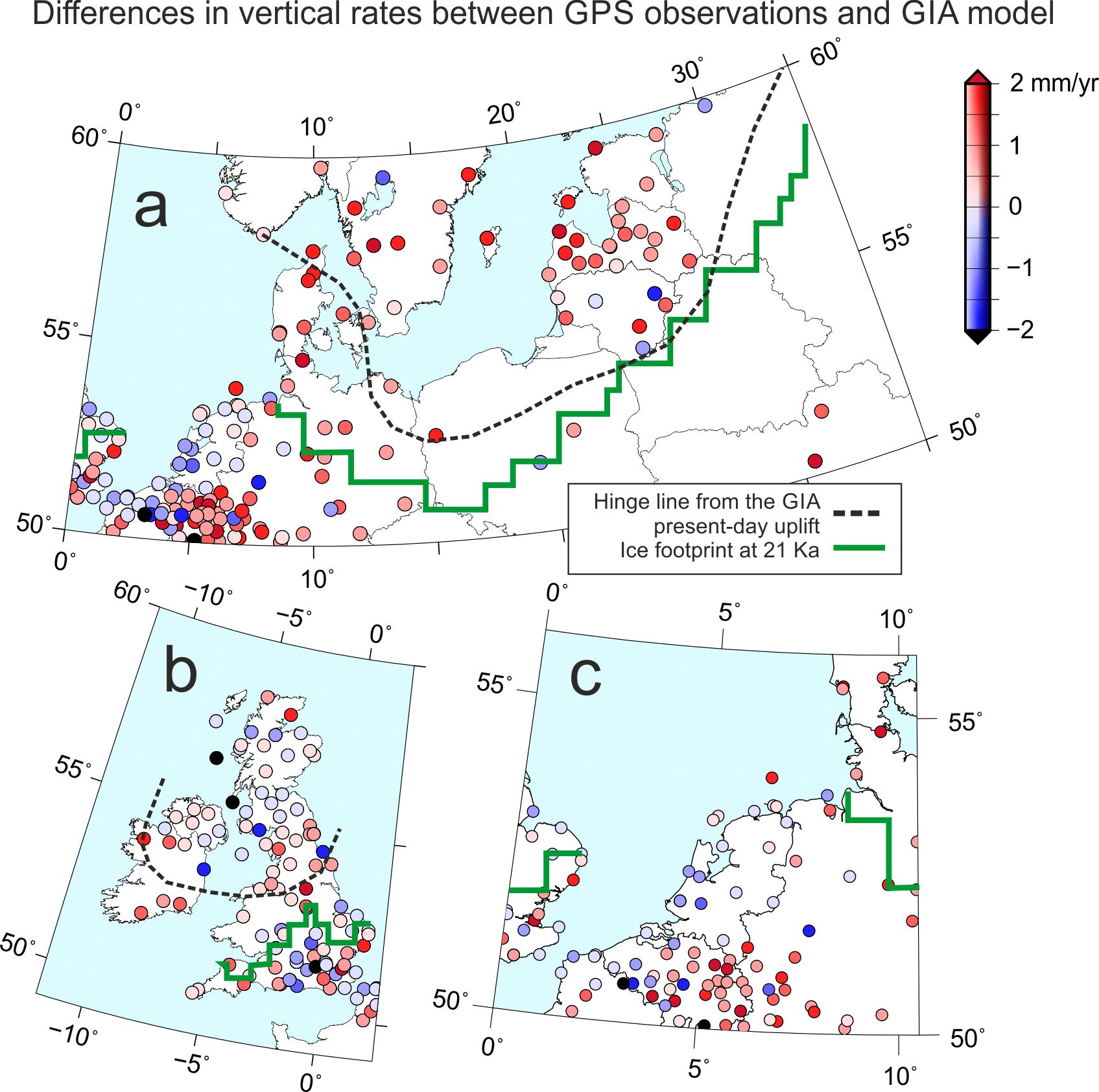
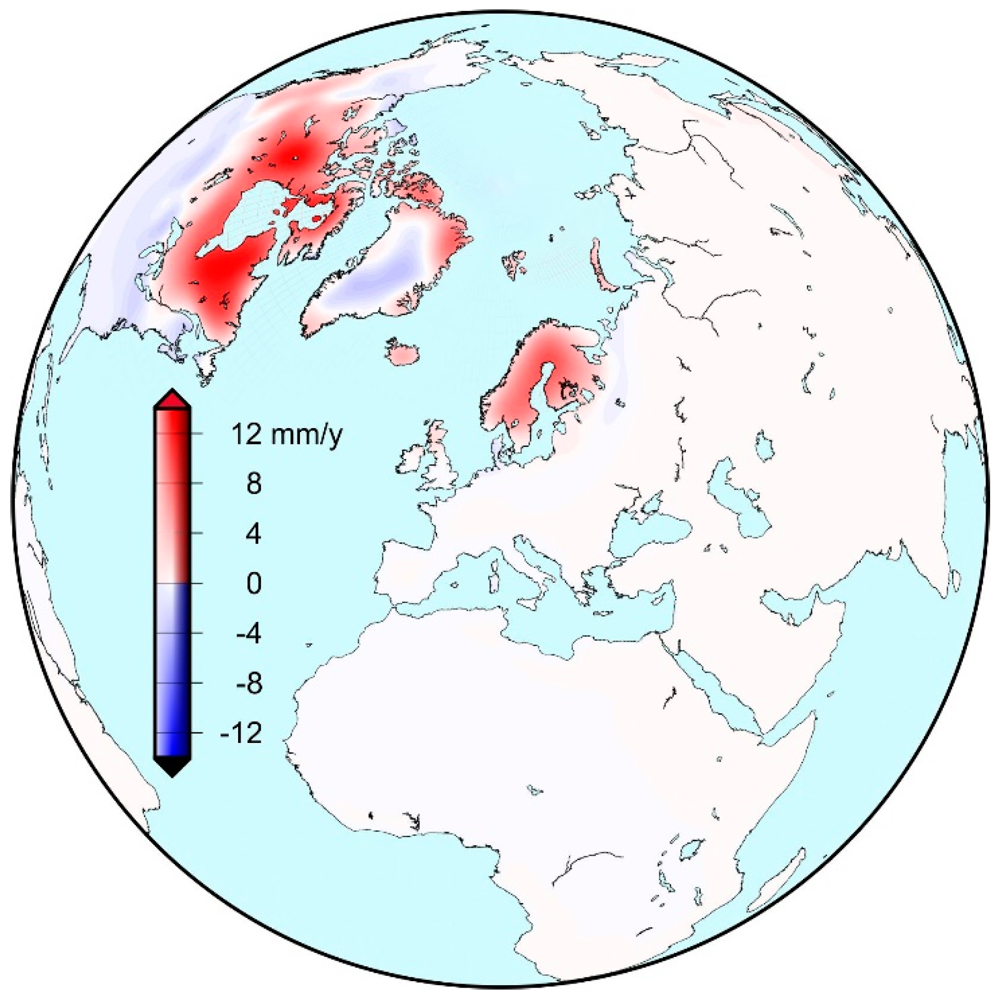
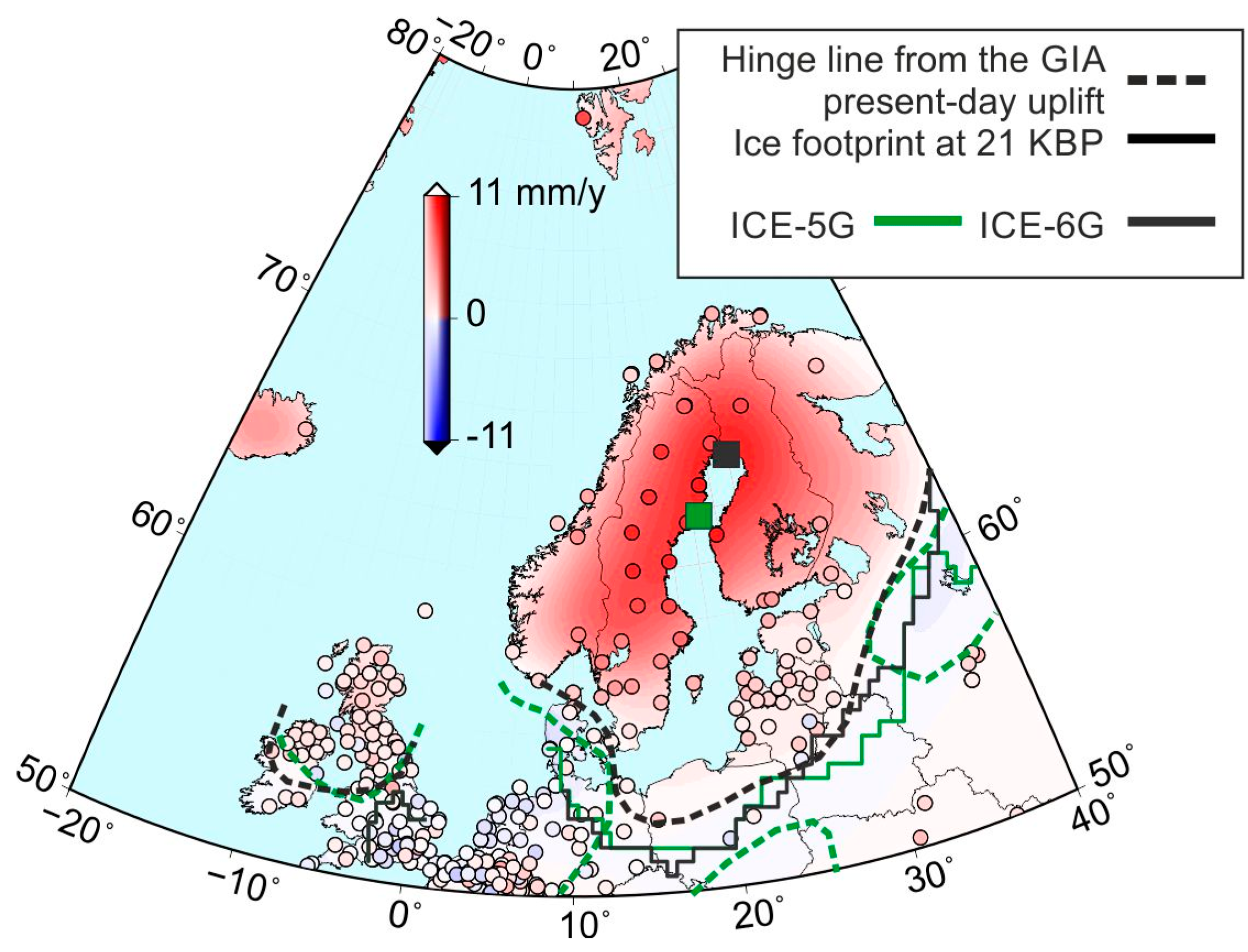
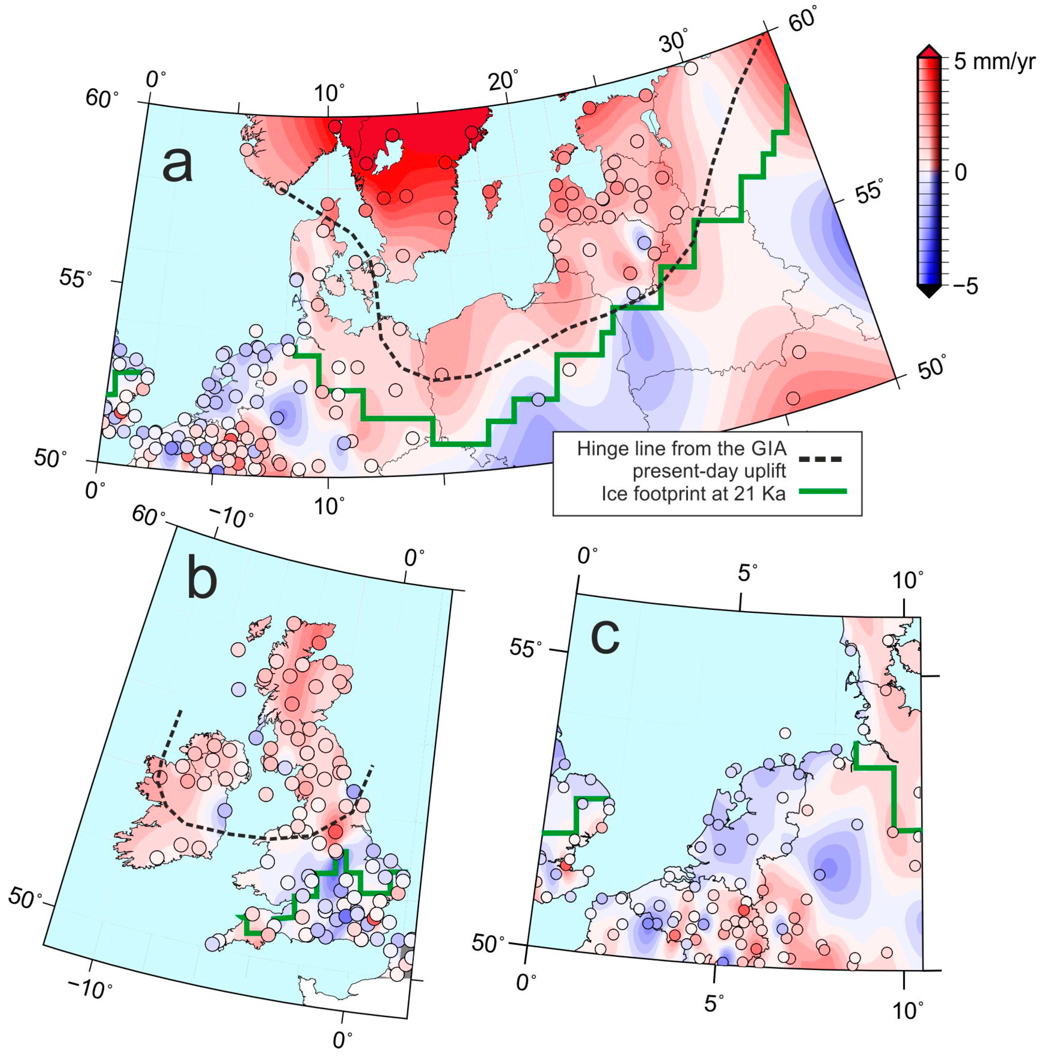
4.4. Comparison to the GIA Model
5. Summary and Conclusions
Supplementary Materials
Author Contributions
Funding
Acknowledgments
Conflicts of Interest
References
- Kreemer, C.; Blewitt, G.; Klein, E.C. A geodetic plate motion and Global Strain Rate Model. Geochem. Geophys. Geosyst. 2014, 15, 3849–3889. [Google Scholar] [CrossRef]
- Yu, S.-B.; Hsu, Y.-J.; Kuo, L.-C.; Chen, H.-Y. GPS measurement of postseismic deformation following the 1999 Chi-Chi, Taiwan, earthquake. J. Geophys. Res. 2003, 108. [Google Scholar] [CrossRef]
- Métivier, L.; Colllieux, X.; Lercier, D.; Altamimi, Z.; Beauducel, F. Global coseismic deformations, GNSS time series analysis, and earthquake scaling laws. J. Geophys. Res. Solid Earth 2014, 119, 9095–9109. [Google Scholar] [CrossRef]
- Karegar, M.A.; Dixon, T.H.; Kusche, J.; Chambers, D.P. A new hybrid method for estimating hydrologically induced vertical deformation from GRACE and a hydrological model: An example from central North America. J. Adv. Model. Earth Syst. 2018, 10, 1196–1217. [Google Scholar] [CrossRef]
- Santamaría-Gómez, A.; Gravelle, M.; Collilieux, X.; Guichard, M.; Martín Míguez, B.; Tiphaneau, P.; Wöppelmann, G. Mitigating the effects of vertical land motion in tide gauge records using a state-of-the-art GPS velocity field. Glob. Planet. Chang. 2012, 98–99, 6–17. [Google Scholar] [CrossRef]
- Karegar, M.A.; Dixon, T.H.; Malservisi, R.; Kusche, J.; Engelhart, S.E. Nuisance flooding and relative sea-level rise: The importance of present-day land motion. Sci. Rep. 2017, 7, 11197. [Google Scholar] [CrossRef]
- Montillet, J.-P.; Melbourne, T.I.; Szeliga, W.M. GPS vertical land motion corrections to sea-level rise estimates in the Pacific Northwest. J. Geophys. Res. Oceans 2018, 123, 1196–1212. [Google Scholar] [CrossRef]
- Ostanciaux, E.; Husson, L.; Choblet, G.; Robin, C.; Pedoja, K. Present-day trends of vertical ground motion along the coast lines. Earth Sci. Rev. 2012, 110, 74–92. [Google Scholar] [CrossRef]
- Bogusz, J. Geodetic aspects of GPS permanent station non-linearity studies. Acta Geodyn. Geomater. 2015, 12, 323–333. [Google Scholar] [CrossRef]
- Bogusz, J.; Klos, A. On the significance of periodic signals in noise analysis of GPS station coordinates time series. GPS Solut. 2016, 20, 655–664. [Google Scholar] [CrossRef]
- Gazeaux, J.; Williams, S.; King, M.; Bos, M.; Dach, R.; Deo, M.; Moore, A.W.; Ostini, L.; Petrie, E.; Roggero, M.; et al. Detecting offsets in GPS time series: First results from the detection of offsets in GPS experiment. J. Geophys. Res. Solid Earth 2013, 118, 2397–2407. [Google Scholar] [CrossRef]
- Williams, S.D.P. The effect of coloured noise on the uncertainties of rates estimated from geodetic time series. J. Geod. 2003, 76, 483–494. [Google Scholar] [CrossRef]
- Graham, S.E.; Loveless, J.P.; Meade, B.J. Global plate motions and earthquake cycle effects. Geochem. Geophys. Geosyst. 2018, 19, 2032–2048. [Google Scholar] [CrossRef]
- Clarke, D.; Brenguier, F.; Froger, J.-L.; Shapiro, N.M.; Peltier, A.; Staudacher, T. Timing of a large volcanic flank movement at Piton de la Fournaise Volcano using noise-based seismic monitoring and ground deformation measurements. Geophys. J. Int. 2013, 195, 1132–1140. [Google Scholar] [CrossRef]
- Henderson, S.T.; Pritchard, M.E. Time-dependent deformation of Uturuncu volcano, Bolivia, constrained by GPS and InSAR measurements and implications for source models. Geosphere 2017, 13, 1834–1854. [Google Scholar] [CrossRef]
- Altamimi, Z.; Rebischung, P.; Métivier, L.; Collilieux, X. ITRF2014: A new release of the International Terrestrial Reference Frame modeling nonlinear station motions. J. Geophys. Res. Solid Earth 2016, 121, 6109–6131. [Google Scholar] [CrossRef]
- Jiang, W.; Li, Z.; van Dam, T.; Ding, W. Comparative analysis of different environmental loading methods and their impacts on the GPS height time series. J. Geod. 2013, 87, 687–703. [Google Scholar] [CrossRef]
- Klos, A.; Gruszczynska, M.; Bos, M.S.; Boy, J.-P.; Bogusz, J. Estimates of Vertical Velocity Errors for IGS ITRF2014 Stations by Applying the Improved Singular Spectrum Analysis Method and Environmental Loading Models. Pure Appl. Geophys. 2018, 175, 1823–1840. [Google Scholar] [CrossRef]
- Ray, J.; Altamimi, Z.; Collilieux, X.; van Dam, T. Anomalous harmonics in the spectra of GPS position estimates. GPS Solut. 2008, 12, 55–64. [Google Scholar] [CrossRef]
- Amiri-Simkooei, A.R.; Mohammadloo, T.H.; Argus, D.F. Multivariate analysis of GPS position time series of JPL second reprocessing campaign. J. Geod. 2017, 91, 685–704. [Google Scholar] [CrossRef]
- Williams, S.D.P.; Bock, Y.; Fang, P.; Jamason, P.; Nikolaidis, R.M.; Prawirodirdjo, L.; Miller, M.; Johnson, D.J. Error analysis of continuous GPS position time series. J. Geophys. Res. 2004, 109, B03412. [Google Scholar] [CrossRef]
- Santamaría-Gómez, A.; Bouin, M.-N.; Collilieux, X.; Wöppelmann, G. Correlated errors in GPS position time series: Implications for velocity estimates. J. Geophys. Res. 2011, 116, B01405. [Google Scholar] [CrossRef]
- Klos, A.; Bogusz, J. An evaluation of velocity estimates with a correlated noise: Case study of IGS ITRF2014 European stations. Acta Geodyn. Geomater. 2017, 14, 261–271. [Google Scholar] [CrossRef]
- Beavan, J. Noise properties of continuous GPS data from concrete pillar geodetic monuments in New Zealand and comparison with data from U.S. deep drilled braced monuments. J. Geophys. Res. 2005, 110, B08410. [Google Scholar] [CrossRef]
- King, M.A.; Bevis, M.; Wilson, T.; Johns, B.; Blume, F. Monument-antenna effects on GPS coordinate time series with application to vertical rates in Antarctica. J. Geod. 2012, 86, 53–63. [Google Scholar] [CrossRef]
- Dong, D.; Fang, P.; Bock, Y.; Cheng, M.K.; Miyazaki, S. Anatomy of apparent seasonal variations from GPS-derived site position time series. J. Geophys. Res. 2002, 107, ETG 9-1–ETG 9-16. [Google Scholar] [CrossRef]
- Bogusz, J.; Gruszczynski, M.; Figurski, M.; Klos, A. Spatio-temporal filtering for determination of common mode error in regional GNSS networks. Open Geosci. 2015, 7, 140–148. [Google Scholar] [CrossRef]
- Gruszczynski, M.; Klos, A.; Bogusz, J. A filtering of incomplete GNSS position time series with probabilistic principal component analysis. Pure Appl. Geophys. 2018, 175, 1841–1867. [Google Scholar] [CrossRef]
- Klos, A.; Bogusz, J.; Figurski, M.; Gruszczynski, M. Error analysis for European IGS stations. Stud. Geophys. Geod. 2016, 60, 17–34. [Google Scholar] [CrossRef]
- Blewitt, G.; Lavallée, D. Effect of annual signals on geodetic velocity. J. Geophys. Res. 2002, 107, ETG 9-1–ETG 9-11. [Google Scholar] [CrossRef]
- Bos, M.S.; Bastos, L.; Fernandes, R.M.S. The influence of seasonal signals on the estimation of the tectonic motion in short continuous GPS time-series. J. Geodyn. 2010, 49, 205–209. [Google Scholar] [CrossRef]
- Klos, A.; Olivares, G.; Teferle, F.N.; Hunegnaw, A.; Bogusz, J. On the combined effect of periodic signals and colored noise on velocity uncertainties. GPS Solut. 2018, 22, 1. [Google Scholar] [CrossRef]
- Steffen, H.; Wu, P.; Wang, H. Optimal locations of sea-level indicators in glacial isostatic adjustment investigations. Solid Earth 2014, 5, 511–521. [Google Scholar] [CrossRef]
- Kuo, C.Y.; Shum, C.K.; Braun, A.; Cheng, K.C.; Yi, Y. Vertical motion determined using satellite altimetry and tide gauges. Terr. Atmos. Ocean. Sci. 2008, 19, 21–35. [Google Scholar] [CrossRef]
- Olsson, P.-A.; Agren, J.; Scherneck, H.-G. Modelling of the GIA-induced surface gravity change over Fennoscandia. J. Geodyn. 2012, 61, 12–22. [Google Scholar] [CrossRef][Green Version]
- Steffen, H.; Wu, P. Glacial isostatic adjustment in Fennoscandia—A review of data and modeling. J. Geodyn. 2011, 52, 169–204. [Google Scholar] [CrossRef]
- Kierulf, H.P.; Steffen, H.; Simpson, M.J.R.; Lidberg, M.; Wu, P.; Wang, H. A GPS velocity field for Fennoscandia and a consistent comparison to glacial isostatic adjustment models. J. Geophys. Res. Solid Earth 2014, 119, 6613–6629. [Google Scholar] [CrossRef]
- Schumacher, M.; King, M.A.; Rougier, J.; Sha, Z.; Khan, S.A.; Bamber, J.L. A new global GPS data set for testing and improving modelled GIA uplift rates. Geophys. J. Int. 2018, 214, 2164–2176. [Google Scholar] [CrossRef]
- Larson, K.M.; van Dam, T. Measuring postglacial rebound with GPS and absolute gravity. Geophys. Res. Lett. 2000, 27, 3925–3928. [Google Scholar] [CrossRef]
- King, M.A.; Santamaría-Gómez, A. Ongoing deformation of Antarctica following recent Great Earthquakes. Geophys. Res. Lett. 2016, 43, 1918–1927. [Google Scholar] [CrossRef]
- Kowalczyk, K.; Bogusz, J. Application of PPP solution to determine the absolute vertical crustal movements: Case study for northeastern Europe. In Proceedings of the 10th International Conference “Environmental Engineering”, Vilnius, Lithuania, 27–28 April 2017. [Google Scholar] [CrossRef]
- Lidberg, M.; Johansson, J.M.; Scherneck, H.-G.; Milne, G.A. Recent results based on continuous GPS observations of the GIA process in Fennoscandia from BIFROST. J. Geodyn. 2010, 50, 8–18. [Google Scholar] [CrossRef]
- Peltier, W.R.; Argus, D.F.; Drummond, R. Space geodesy constraints ice age terminal deglaciation: The global ICE-6G_C (VM5a) model. J. Geophys. Res. Solid Earth 2015, 120, 450–487. [Google Scholar] [CrossRef]
- Zumberge, J.F.; Heflin, M.B.; Jefferson, D.C.; Watkins, M.M.; Webb, F.H. Precise point positioning for the efficient and robust analysis of GPS data from large networks. J. Geophys. Res. Solid Earth 1997, 102, 5005–5017. [Google Scholar] [CrossRef]
- Blewitt, G.; Kreemer, C.; Hammond, W.C.; Goldfarb, J.M. Terrestrial reference frame NA12 for crustal deformation studies in North America. J. Geodyn. 2013, 72, 11–24. [Google Scholar] [CrossRef]
- Kaplon, J.; Kontny, B.; Grzempowski, P.; Schenk, V.; Schenkova, Z.; Balek, J.; Holesovsky, J. GEOSUD/SUDETEN network GPS data reprocessing and horizontal site velocity estimation. Acta Geodyn. Geomater. 2014, 11, 65–75. [Google Scholar] [CrossRef]
- Walo, J.; Prochniewicz, D.; Olszak, T.; Pachuta, A.; Andrasik, E.; Szpunar, R. Geodynamic studies in the Pieniny Klippen Belt in 2004–2015. Acta Geodyn. Geomater. 2016, 13, 351–361. [Google Scholar] [CrossRef]
- Bos, M.S.; Fernandes, R.M.S.; Williams, S.D.P.; Bastos, L. Fast error analysis of continuous GNSS observations with missing data. J. Geod. 2013, 87, 351–360. [Google Scholar] [CrossRef]
- Peltier, W.R. Global Glacial Isostasy and the Surface of the Ice-Age Earth: The ICE-5G(VM2) model and GRACE. Ann. Rev. Earth Planet. Sci. 2004, 32, 111–149. [Google Scholar] [CrossRef]
- Argus, D.F.; Peltier, W.R.; Drummond, R.; Moore, A.W. The Antarctic component of postglacial rebound Model ICE-6G_C(VM5a) based upon GPS positioning, exposure age dating of ice thicknesses and sea level histories. Geophys. J. Int. 2014, 198, 537–563. [Google Scholar] [CrossRef]
- Klos, A.; Bogusz, J.; Moreaux, G. Stochastic models in the DORIS position time series: Estimates for IDS contribution to ITRF2014. J. Geod. 2018, 92, 743–763. [Google Scholar] [CrossRef]
- Langbein, J.; Johnson, H. Correlated errors in geodetic time series: Implications for time-dependent deformation. J. Geophys. Res. 1997, 102, 591–603. [Google Scholar] [CrossRef]
- Schwarz, G.E. Estimating the dimension of a model. Ann. Stat. 1978, 6, 461–464. [Google Scholar] [CrossRef]
- Zhang, J.; Bock, Y.; Johnson, H.; Fang, P.; Williams, S.; Genrich, J.; Wdowinski, S.; Behr, J. Southern Californnia permanent GPS geodetic array: Error analysis of daily position estimates and site velocities. J. Geophys. Res. 1997, 102, 18035–18055. [Google Scholar] [CrossRef]
- Bos, M.S.; Fernandes, R.M.S.; Williams, S.D.P.; Bastos, L. Fast error analysis of continuous GPS observations. J. Geod. 2008, 82, 157–166. [Google Scholar] [CrossRef]
- Simon, K.M.; Riva, R.E.M.; Kleinherenbrink, M.; Frederikse, T. The glacial isostatic adjustment signal at present day in northern Europe and the British Isles estimated from geodetic observations and geophysical models. Solid Earth 2018, 9, 777–795. [Google Scholar] [CrossRef]
- Bos, M.S.; Williams, S.D.P.; Araújo, I.B.; Bastos, L. The effect of temporal correlated noise on the sea level rate and acceleration uncertainty. Geophys. J. Int. 2013, 196, 1423–1430. [Google Scholar] [CrossRef]
- Rajner, M. Detection of ice mass variation using GNSS measurements at Svalbard. J. Geodyn. 2018, 121, 20–25. [Google Scholar] [CrossRef]
- Klos, A.; Bogusz, J.; Figurski, M.; Kosek, W. Irregular variations in GPS time series by probability and noise analysis. Surv. Rev. 2015, 47, 163–173. [Google Scholar] [CrossRef]
- Van der Wal, W.; Whitehouse, P.L.; Schrama, E.J.O. Effect of GIA models with 3D composite mantle viscosity on GRACE mass balance estimates for Antarctica. Earth Planet. Sci. Lett. 2015, 414, 134–143. [Google Scholar] [CrossRef]
- Nocquet, J.-M.; Sue, C.; Walpersdorf, A.; Tran, T.; Lenotre, N.; Vernant, P.; Cushing, M.; Jouanne, F.; Masson, F.; Baize, S.; et al. Present-day uplift of the western Alps. Sci. Rep. 2016, 6, 28404. [Google Scholar] [CrossRef]


© 2019 by the authors. Licensee MDPI, Basel, Switzerland. This article is an open access article distributed under the terms and conditions of the Creative Commons Attribution (CC BY) license (http://creativecommons.org/licenses/by/4.0/).
Share and Cite
Bogusz, J.; Klos, A.; Pokonieczny, K. Optimal Strategy of a GPS Position Time Series Analysis for Post-Glacial Rebound Investigation in Europe. Remote Sens. 2019, 11, 1209. https://doi.org/10.3390/rs11101209
Bogusz J, Klos A, Pokonieczny K. Optimal Strategy of a GPS Position Time Series Analysis for Post-Glacial Rebound Investigation in Europe. Remote Sensing. 2019; 11(10):1209. https://doi.org/10.3390/rs11101209
Chicago/Turabian StyleBogusz, Janusz, Anna Klos, and Krzysztof Pokonieczny. 2019. "Optimal Strategy of a GPS Position Time Series Analysis for Post-Glacial Rebound Investigation in Europe" Remote Sensing 11, no. 10: 1209. https://doi.org/10.3390/rs11101209
APA StyleBogusz, J., Klos, A., & Pokonieczny, K. (2019). Optimal Strategy of a GPS Position Time Series Analysis for Post-Glacial Rebound Investigation in Europe. Remote Sensing, 11(10), 1209. https://doi.org/10.3390/rs11101209