Article

Optical and SAR Remote Sensing Synergism for Mapping Vegetation Types in the Endangered Cerrado/Amazon Ecotone of Nova Mutum—Mato Grosso

1
Physical Geography Department, University of Göttingen, Goldschmidtstr. 5, 37077 Göttingen, Germany
2
Landesamt für Vermessung und Geoinformation Schleswig-Holstein, Dezernat 22, Mercatorstraße 1, 24106 Kiel, Germany
3
Forest Engineering Department, Santa Catarina State University, Av. Luiz de Camões 2090, 88.520-000 Lages, Santa Catarina, Brazil
4
Cartography, GIS & Remote Sensing Department, University of Göttingen, Goldschmidtstr. 5, 37077 Göttingen, Germany
*
Author to whom correspondence should be addressed.
Remote Sens. 2019, 11(10), 1161; https://doi.org/10.3390/rs11101161
Submission received: 18 April 2019 / Revised: 8 May 2019 / Accepted: 10 May 2019 / Published: 15 May 2019
(This article belongs to the Special Issue Remote Sensing of Savannas and Woodlands)

Abstract

:
Mapping vegetation types through remote sensing images has proved to be effective, especially in large biomes, such as the Brazilian Cerrado, which plays an important role in the context of management and conservation at the agricultural frontier of the Amazon. We tested several combinations of optical and radar images to identify the four dominant vegetation types that are prevalent in the Cerrado area (i.e., cerrado denso, cerradão, gallery forest, and secondary forest). We extracted features from both sources of data such as intensity, grey level co-occurrence matrix, coherence, and polarimetric decompositions using Sentinel 2A, Sentinel 1A, ALOS-PALSAR 2 dual/full polarimetric, and TanDEM-X images during the dry and rainy season of 2017. In order to normalize the analysis of these features, we used principal component analysis and subsequently applied the Random Forest algorithm to evaluate the classification of vegetation types. During the dry season, the overall accuracy ranged from 48 to 83%, and during the dry and rainy seasons it ranged from 41 up to 82%. The classification using Sentinel 2A images during the dry season resulted in the highest overall accuracy and kappa values, followed by the classification that used images from all sensors during the dry and rainy season. Optical images during the dry season were sufficient to map the different types of vegetation in our study area.

1. Introduction

The Cerrado biome is considered as being among the most extensive and diverse ecosystems in the Neotropics and is a hotspot in the context of biodiversity [1]. It is also one of the most threatened ecosystems in South America, with over 40% of the biome converted to agriculture and the remainder highly fragmented [2]. Despite the threat to the Brazilian Cerrado, studies on this ecosystem are few and recent.
The Cerrado biome is the second largest complex vegetation present in Brazil and occupies about 200 million hectares, of which the largest territory is in the state of Mato Grosso [3]. This large distribution of the Cerrado biome in Brazil covers three main vegetation types: grassland, savannas, and forest formations, which results in indeterminate boundary and a gradient of biomass, height, and tree cover. This large variance in different types of vegetation in the Cerrado is responsible for the high biodiversity in this biome. The three areas of biodiversity in Cerrado, the South–Southeast, Central Plateau, and Northeast areas are mainly separated by the altitude and latitude [4]. The heterogeneity of the vegetation types is also seen in the microclimate variability and in different types of soils, e.g., mostly latosol, red-yellow latosol, red latosol, quartz-neosols, and argisols [5,6,7]. In addition, the amount of biomass and carbon storage is differently distributed in the biome, depending on the vegetation type and soil [8,9,10]. This large biodiversity and floristic heterogeneity in Cerrado was and is decreasing due to deforestation since the 1980s, which can lead to a loss or decrease in ecosystem services [11].
Cerrado is the most deforested biome in Brazil due to the high agricultural impact, particularly caused by the world market-oriented production of soy, cotton, and sugarcane. Deforestation is facilitated by its flat topography, easy management of the soil for agricultural activities, and high mechanization [12]. For pasture and agricultural activities, Cerrado has become a more viable alternative to the Amazon despite its poor soil quality. Despite a lack of consistent deforestation records, a few studies have looked at rates of deforestation in the Cerrado biome. Machado et al. [13] analyzed the deforestation rates from two different sources. They found that from 1985 to 1993, Cerrado lost 1.5% of its total vegetation area annually. From 1993 to 2002, the rate of deforestation per year decreased to 0.67%. Starting from 2002, several Brazilians institutes, such as the Instituto Brasileiro do Meio Ambiente e dos Recursos Naturais Renováveis (IBAMA) and National Institute for Space Research (INPE), started to monitor the rate of deforestation in the Cerrado biome. From 2002 to 2017, Cerrado lost around 0.8% of its total vegetation area per year. The ease of deforesting in the Cerrado biome created a hotspot region for deforestation at the boundary with Amazon biomes.
Current regulation and restrictions in ecosystem preservation have driven deforestation and cover changes into the forest–savanna transition zone, as in West Africa [14] and South America [15]. Janssen at al. [14] projected an increase of tree cover losses from 20 to 85% in Ghana. In South America, the transitional zone is known as “arc of the deforestation” (AOD). The AOD is located in the frontier states of Mato Grosso, Pará, and Rondônia, and it accounts for 85% of the areas that were deforested between 1996 to 2005 [16,17]. In these transition areas, the laws that support the protection of forests are even weaker and unmanaged. One example is the environmental legislation that defines the amount of natural vegetation that has to be preserved (80% in the Amazon, 20% in the Cerrado biome) [18]. Additionally, this forest–savanna boundary comprises a mixture of floristic characteristics from both adjacent regions, which increases the complexity in mapping the ecotone between the Amazon and Cerrado. Marques et al. [19] showed that the official boundary between Cerrado and Amazon conducted by the Brazilian Institute of Geography and Statistics (IBGE) is not accurate, and in some areas, the length of the transition zone was miscalculated by 245.5%. This problem is likely to misinterpret the mapping of land use and consequently decrease the accuracy of vegetation classification. Moreover, the problem of low accuracy in the mapping of the boundary between Cerrado and Amazon affects the calculation of wood density, and therefore biomass estimation as well [20]. To overcome these problems, Brazil needs to improve the monitoring system of deforestation and land use change (LUC), especially for the Cerrado biome.
The field monitoring of Cerrado is a time-consuming challenge, given the large size of the biome. Hence, the use of remote sensing facilitates the monitoring of the status and changes in land cover and land use at large scales. Most studies with remote sensing to monitor the differentiation of the vegetation types in Cerrado use optical sensors, mainly in the savanna and grassland formations where there is low signal saturation. These studies mostly use the Normalized Difference Vegetation Index (NDVI) [21,22,23], Spectral Linear Mixture Model (SLMM) [24,25], and phenological profiles [26]. Additionally, Müller et al. [27] demonstrated the challenges in mapping land use in Cerrado, essentially a result of its high diversity. The study showed a considerable uncertainty in the classification of cropland and pastures areas. The same problem was reported by Sano et al. [28], whose study reports a spectral similarity between cropland, pasture, and natural savanna vegetation, which can increase the uncertainty when mapping. Moreover, Ministry of the Environment (MMA) [29] mapped the land use in the whole Cerrado biome and the study showed that one of the biggest challenges for this area was to map the different types of vegetation, due to the strong seasonality of natural vegetation. However, the optical sensors can extract the information from the canopy, but arboreal vegetation types have differences in vertical structure and tree cover, so that with optical sensors, uncertainties in the identification of forest savanna vegetation types increase. Additionally, optical images are affected by weather conditions (cloud cover).
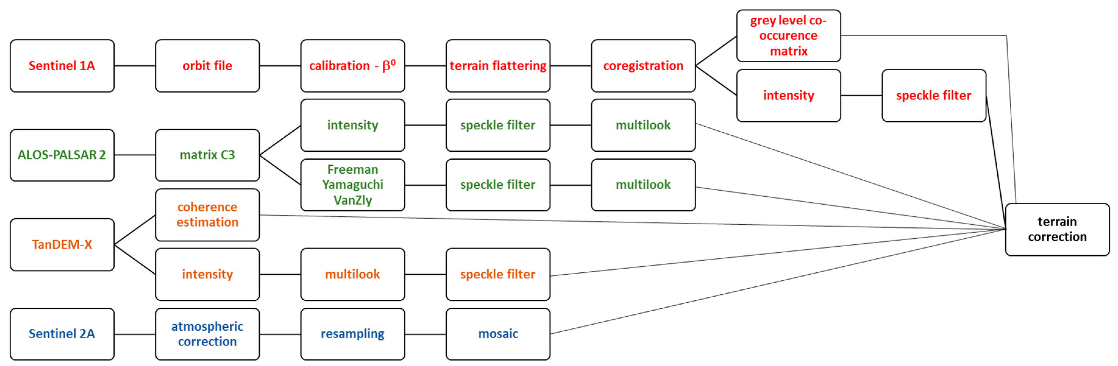
Radar sensors have an important advantage compared to optical sensors: the ability of radiation to penetrate through cloud cover and considerable parts of the canopy of trees/forest stands due to the higher wavelengths compared to optical sensors. Thus, the resulting radar signals (amplitude/backscatter and, if available, coherence) provide information that can be used to describe the vertical structure of vegetation stands. This information can be used to better estimate forest structure variables such as canopy cover, tree density, tree height or others, as well as to stratify vegetation (e.g., different types of forest). The longer the wavelength, the deeper radar Bands penetrate dense vegetation, which increases its sensibility to perceive the differences that improve discrimination of vegetation types. Almeida-Filho and Shimabukuro [30] demonstrated that the L Band from the JERS-1 synthetic-aperture radar (SAR) can be used to detect cover changes in forested and non-forested areas in the Cerrado biome. Evans and Costa [31] also mapped six vegetation habitats in Brazil using L and C Bands using the backscattering information from the surface. In the same country, Saatchi et al. [32] mapped five land cover types using the JERS-1 mosaic, using texture measurement. Santos et al. [33], Sano et al. [34], and Mesquita et al. [35] had satisfactory results using radar images to discriminate the vegetation types in the Cerrado biome, especially with the L Band. The sensitivity of the radar sensor to perceive the differences in vegetation structures makes it useful for mapping different types of forests.
The savanna vegetation has one of the largest forest diversities. In this case, the combination of different satellite images (optical and radar) and spatial resolution (low, medium, and high) may help to improve the quality of satellite based monitoring concepts [32]. However, there is little information about how the synergy of different data can contribute to map forest vegetation types in Cerrado. Yet, the free availability and the development of new optical and radar sensors, such as Sentinel 2A, Sentinel 1A (both free) or ALOS2 and TanDEM-X, are increasing the use of both sensors (radar and optical) for vegetation mapping. Recent studies have shown that the synergy of radar and optical images improved vegetation type discrimination, especially in the Cerrado biome, where the greenness seasonality had a huge influence during the year [36,37,38].
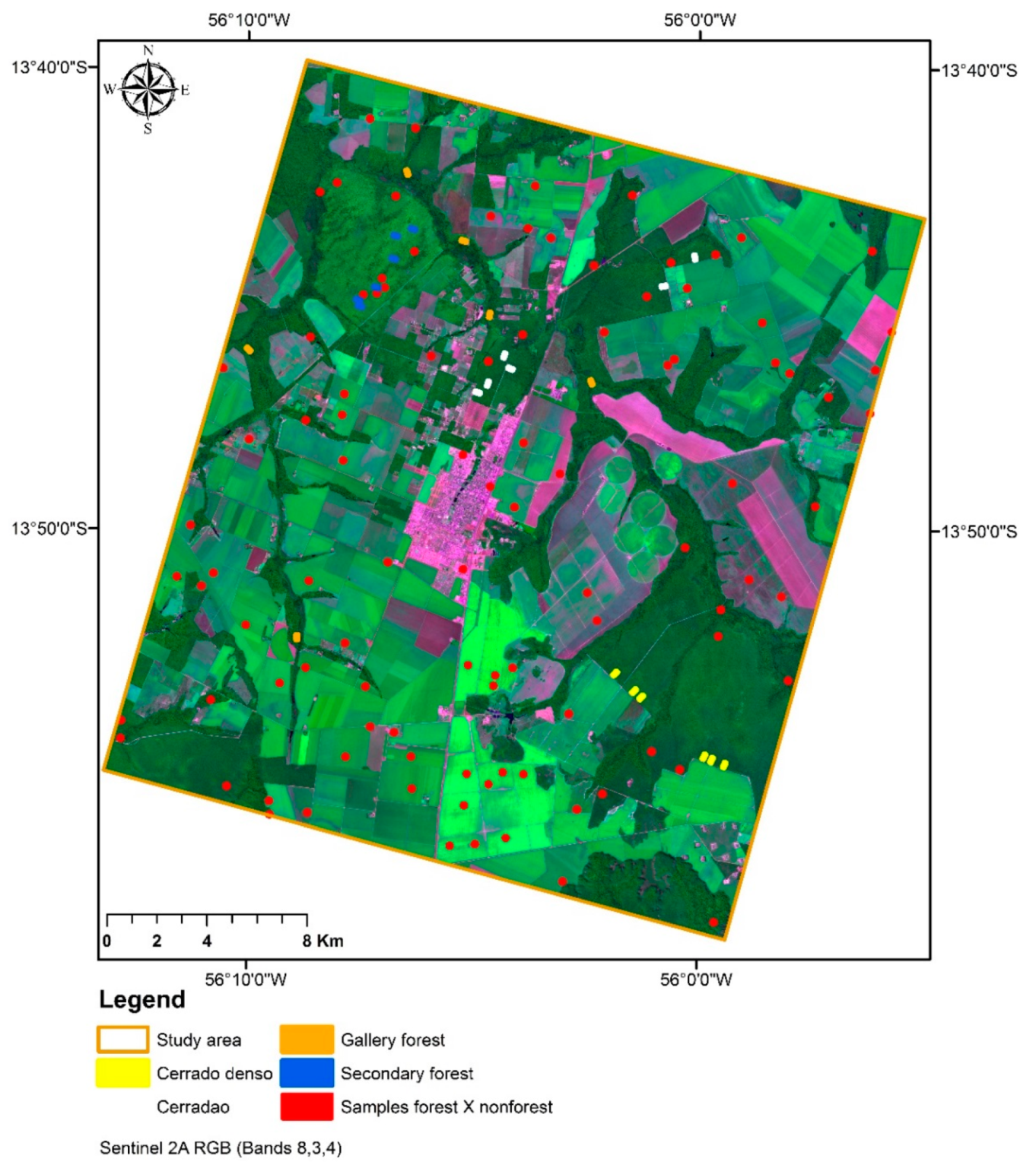
The aforementioned studies concentrate on parts of Cerrado where the vegetation cover is mostly homogeneous and that are not located in transitional areas such as the the Arc of Deforestation. However, most of the deforestation and expansion of agricultural and pasture areas are concentrated in this region. Additionally, these regions have a mixture of vegetation type and species from Cerrado and Amazon, which makes the study in this area more complex. The few studies in this area are related to the land use and not the mapping of vegetation type, as in Zaiatz et al. [39], who evaluated the spatial and temporal dynamics of land use and cover of the Upper Teles Pires River Basin from 1986 to 2014. In order to overcome the lack of studies using both sensors to discriminate vegetation types, the aim of this study is to evaluate the use of optical and radar remote sensing for mapping the different types of vegetation in the transitional area between the Cerrado and Amazon biomes.

2. Materials and Methods

2.1. Study Sites

The study area was the result of an overlap between the satellite images selected for this study and it is located around the city of Nova Mutum, Mato Grosso, which includes the Cerrado and Amazon biomes. Nova Mutum is located in the north of Mato Grosso, Brazil, and it is part of the Alto Teles Pires River Basin (Figure 1). Its climate is classified as Aw (after the Köppen climate classification), with a clear seasonality of rainy season (October to April) and dry season (May to September). The annual average temperature is 24 °C and annual precipitation is approximately 2200 mm [40]. The topography is flat with maximum slopes of 3%. The soils in the the area are Oxisols (80%) and Entisols (20%) [41].
Nova Mutum is located in the AOD; this area covers 256 municipalities with the most intensive deforestation activities in an area of approximately 1,700,000 km2 and it plays an important role in the context of deforestation in the frontier of Amazon and Cerrado. The AOD accounts for 75% of the deforestation in the Brazilian Amazon and the largest agricultural area [17]. Legislation, soil, relief, climate conditions, and the subsidies offered by the government have encouraged agricultural activity since 1970. Recently, the Brazilian government has established policies to decrease the rates of deforestation in these areas, such as the “Soy Moratorium” [42], which was an agreement with the major soybean traders not to purchase soybean that was planted in deforested areas after July 2006 in the Brazilian Amazon biome.
In general, the vegetation of Cerrado in Brazil covers three main different vegetation types: grassland, savannas, and forest formations. The forest formations consist of arboreal species in a continuous canopy and include the Gallery, Dry, and Open Forest. The savanna formation is characterized by a discontinuous herbaceous-shrub and tree canopy. The seven types of savanna formation are Dense Woodland, Woodland, Open Woodland, Park Woodland, Palm, Vereda, and Stone Woodland. The grassland formations include three vegetation types: Stone Grassland, Shrub Savanna, and Grassland. The first two types of grasslands are characterized by the large presence of shrubs with different types of soils. Figure 2 summarizes the distribution of the three different vegetation formations in the Cerrado biome. Each of these types has a high diversity, which is a consequence of the high variability of the soil and microclimates as well as the floristic evolution with plants from different Brazilian biomes [7].
In our study, we mapped the four dominating vegetation types in Nova Mutum, cerradão (Open Forest), cerrado denso (Dense Woodland), gallery forest, and secondary forest. Cerradão and cerrado denso are located within the transition area of the Amazon and Cerrado biomes. As mentioned before, this area has a high deforestation rate, which can explain the presence of secondary forest. Cerradão has a crown cover between 50 and 90% and the height of the trees varies from 8 to 15 m. In general, the soils of Cerradão are well drained, deep, and have medium–low fertility. Cerrado denso has a crown cover between 5 to 70% and tree height varies from 5 to 8 m. The layers of shrubs and herbs are less dense compared to cerradão. In general, the soils of cerrado denso have medium to very clayey texture and are middle-well drained. The gallery forest has a crown cover between 70 to 95% and the height of the trees varies from 20 to 30 m. Secondary forests are formed after clear-cutting and have different structures, depending on the age of the succession. At the beginning of its succession time, these secondary forests are poor in biodiversity and have a simple structure, whereas in the next succession time, its structure depends on environmental factors such as soil, climate, and management [44].

2.2. Satellite Data

In order to analyze the use of optical and radar sensors to map the vegetation type in Cerrado, we used a set of images from four sensors (3 SARs and 1 optical). The PALSAR-2 aboard ALOS-2 from the Japan Aerospace Exploration Agency (JAXA); TanDEM-X (TerraSAR-X add-on for Digital Elevation Measurement) from the German Aerospace Center, DLR, and Astrium GmbH; Sentinel 1A and the optical Sentinel 2A from the European Union’s Copernicus programme. Figure 3 shows the temporal coverage of each satellite image used in our analysis.
We selected the satellite image data following some criteria. First, we selected images from 2017 since the field data were collected in 2017, except for the TanDEM-X image. Secondly, we selected the radar images on the dates of low precipitation, prior to the date of acquisition. Table 1 shows the date, polarization, orbit, and accumulated precipitation values three days before the acquisitions.

2.3. Data Processing

2.3.1. Sentinel 2A

Seven coverages (using nine Bands altogether, from Band 2 to Band 8A, Band 11, and Band 12) of the Multispectral Instrument (MSI) on-board Sentinel-2A were processed using the ESA’s Sentinel-2 toolbox in the ESA Sentinel Application Platform (SNAP). First, we applied atmospheric correction using Sen2cor, which is a L2A-processor for Sentinel-2 data that creates Bottom-Of-Atmosphere (BOA) reflectance images using Top-Of-Atmosphere (TOA) data [45]. Secondly, we resampled all the bands to a 10-m spatial resolution based on the geolocations obtained from Level-1C metadata. For the last step, we created a subset of our study area to speed up processing time, and lastly we mosaicked the images, as our study area was between two different orbits of the Sentinel 2A.
During the final step, we reduced the number of features by applying principal component analysis (PCA) on the spectral dataset due to the fact that some classification algorithms, such as Random Forest, cannot work well with high correlation data. Principal component analysis is a mathematical procedure that reduces a large amount of variables into principal components. The primary function of the PCA is to determine the extent of the correlation between multispectral bands and to remove it through an appropriate mathematical transformation [46]. We used the first principal component (PC1) of each one of the ten bands to aggregate only information that was essential to the classification process, as it explained most of the variance, e.g., PC1 of Band 2, PC1 of Band 3, and PC1 of Band 4. Overall, this resulted in a set of ten variables as input for classification for the dry season, and the dry and rainy season, respectively.

2.3.2. Sentinel 1A

Twenty-three coverages from Sentinel-1A IW Ground Range Detected (GRD) Level-1 product were processed using the ESA Sentinel Application Platform toolbox. First, each image was radiometrically calibrated to radar brightness values (β0) [47]. Secondly, we applied the terrain flattening to correct any terrain variations in the images. Terrain flattering is an important step for the mapping of land use. Without the terrain flattening, an additional error into the coherency and covariance measurement could be created, due to the difference in the terrain and subsequently the brightness of the radar return [48]. During the third step, we coregistrated the 23 images based on the cross-correlation technique to guarantee that every pixel was correctly located in the same target of all images [49]. Once we had the images from the co-registration process, we separated them into two sub-processes. During the first process, we applied the grey level co-occurrence matrix (GLCM) to extract second order statistical textures features. The GLCMs were extracted separately from every single date and polarization (VV and VH). These textures can be useful to improve land use classification in that it extracts intensity variations from the image involving the information of the neighbor pixels to identify specific clusters or objects [50]. Additionally, we applied the Refined Lee speckle filter (window size 5 × 5), after GLCMs extraction. This process is necessary to reduce the noise caused by random constructive and destructive interference from the radar signal [51]. For the second branch of processing, we only applied the Refined Lee speckle filter on the backscatter images. We applied the Range Doppler terrain correction in the last step. This process is necessary to geocode and correct the distortions in the image, which are caused by the topographical variations and the tilt of the sensor [52]. The entire process is illustrated in Figure 4.
We applied the PCA to reduce the number of features in the same way as explained above for Sentinel 2A. In the backscattering images, we applied the PCA for the two different seasons and two polarizations, which resulted in four PCs: (a) images of VV polarization in the rain and dry season; (b) images of VH polarization in the rain and dry season; (c) images of VV polarization during the dry season; and (d) images of VH polarization during the dry season. The same was applied for the texture images (ten textures: ASM, contrast, correlation, dissimilarity, energy, entropy, homogeneity, MAX, mean, variance. This resulted in a set of twenty two inputs in the dry season (one PC of VV, one PC of VH, ten PCs of VV textures, and ten PCs of VH textures) and a set of fourth four inputs in the rainy and dry season (one PC of VV in the dry season; one PC of VV in the rainy and dry season; one PC of VH in the dry season; one PC of VH in the rainy and dry season; ten PCs of VV textures in the dry season; ten PCs of VV in the rainy and dry season; ten PCs of VH textures in the dry season; ten PCs of VH in the rainy and dry season).

2.3.3. ALOS-PALSAR 2 (Dual and Full Polarimetric)

Four coverages of the dual polarization images were converted to covariance matrix C2 and one coverage of the full polarization images was converted to C3 matrix [53]. In this step, multilook with 4 looks in azimuth and 1 in range was applied to convert the image from single look complex to ground range detected. We applied the speckle filter on all images to reduce speckle noise. For that we used the Refined Lee adaptive filter (5 × 5 window), which is more efficient and whose results have less destructive averaging, having been largely used in the radar studies [51,52,53,54]. Here, we separated the images into two subprocesses. For the first, we kept the backscattering images. For the second, we calculated polarimetric decompositions. Polarimetric SAR decomposition is a useful method to map and discriminate the different targets on the surface, especially due to the signal of the target, which is a combination of speckle noise and random vector scattering effects [55]. In our study, we chose the Freeman–Durden, Yamaguchi, and VanZyl polarimetric decompositions. In general, these three decompositions are based on the covariance matrix that is divided into three scattering mechanism: volume, double bounce and surface scatter [55]. Additionally, polarimetric compositions have been used before in mapping of vegetation showing the improvement in the vegetation classification in the Amazon and Cerrado [56]. We applied the Range Doppler terrain correction in all images.
Following the same process of the other images, we applied the PCA to reduce the number of features and consequently facilitated the further classification process. This resulted in a set of ten PCs, resulting in four of the dual polarimetric, PC1 of backscattering in each polarization (HH and VH) and each orbit (ascending and descending) and six of the full polarimetric: PC1 of backscattering in each polarization (HH, VV and VH) and PC1 of each scattering mechanism (volume, double bounce and surface scatter).

2.3.4. TanDEM-X

The TanDEM-X mission operates two X-Band satellites flying in close formation in order to acquire single-pass interferometric SAR data. The primary mission goal of the TanDEM-X mission was the generation of a global digital elevation model [57]. All TanDEM-X acquisitions are available to the science community on request in Coregistered Single look Slant range Complex (CoSSC) format. For the study area, we acquired one TAnDEM-X scene in standard (bistatic) mode with horizontal polarization (HH). The processed data was separated into two different parts. In the first part, we estimated the magnitude of coherence. Coherence describes the the degree of correlation between the two complex radar images [58]. It is a measure of quality of the phase measurement in interferometric SAR analysis and also used as a proxy for soil and vegetation structural parameters.
In the second part, we processed the intensity images. We performed multilook in both images (coherence and intensity) from the first and second part, with 4 looks in azimuth and 3 in range to reduce the noise. Additionally, we applied, as with the other images before, the speckle filter Refined Lee (window 5 × 5). For the last step, we applied the Range Doppler terrain correction. All images were processed to have a final product with spatial resolution of 10 m. The PCA was not applied for TanDEM-X due to the use of only one single date.

2.4. Classification

The process of image classification was separated into two steps. First, a forest mask was generated as a result of a forest/non-forest classification. At the second step, we classified the forest type within this forest mask. The area under investigation is covered by all images used in this study.
We used the RF algorithm implemented in R software for image classification. Random Forests is a supervised classification algorithm that uses multiples decision trees to get an accurate classification and prediction. The N numbers of trees are being built by the classifier, contributing each to the assignment of the most frequent class. This algorithm uses the bagging method to produce random samples of training sets for each random decision tree. Every tree uses a random subset from the original set. This original set was created from training samples, where two-thirds were used to train the classifier and one-third of them were used for validation. Two-thirds of the training sample were the out-of-bag (OOB) data and one-third of the training sample were the OOB error estimate [59]. Random Forest can be used for classification and regression and is an efficient tool due to measuring the relative importance of each feature. This variable importance measures the decrease of accuracy when a variable is removed from the classification. The higher a variable is ranked, the more it is contributing to the accuracy. Additionally, it has a lower probability to overfit compared to other models if there are enough trees. This method has many improvements: it does not require any input preparation, it is more stable using big data since it works well with variable non-linearity, it provides a pre-feature selection building the trees, and reduces the time required for the process. For remote sensing analysis, RF showed to be a stable and accurate algorithm, especially when it is applied to different types of sensors and large time series. The achievement of this method can be seen in recent studies such as References [59,60,61], which applied RF for vegetation mapping using different types of data. In this study, the RF models consisted of 1000 trees, and 70% of our samples were used for training the classifier and 30% for validation of the classification results.

2.4.1. Forest and Non-Forest

In order to classify the several vegetation types, we first needed to create a map of forest and non-forest areas. For accuracy assessment, we created 100 random points of 3.13 ha each and visually classified them using high-resolution imagery from Google Earth and the sensor Sentinel 2A (Figure 5). During the classification process, we used 70% of these points for training the classifier and 30% for validation of the classification results.

2.4.2. Forest Type

Forest-type mapping was only conducted in the areas masked as forests in the previous step. We created 24 reference areas equally distributed into four different vegetation classes (cerradão, cerrado denso, gallery, and secondary forest). Each one had an area of 14.265 ha (Figure 5). The polygons were classified based on field data collection (July 2017) and high-resolution imagery from Google Earth and Sentinel 2A (26 July 2017). During the classification process using RF, we used 70% of the pixels in the 24 references areas for training and 30% for validation.
To analyze the synergy of optical and radar data for mapping Cerrado vegetation types, all possible combinations between optical and radar sensors were tested in two different scenarios, dry season, dry and rainy seasons (Table 2). In addition, we used the sensors separately and analyzed the SAR classifications. In total, 23 datasets were processed.
For the classifications, which combined two or more sensors, e.g., Sentinel 2A and ALOS-PALSAR 2, we did not use all the features of each sensor. In this case, we selected the first three features based on variable importance, which was calculated during RF classification for the single sensor dataset, respectively. Variable importance shows the interaction between the variables/features and inserts them into an hierarchy within a level of contribution and importance for the classification.
For both classifications, forest/non-forest and vegetation type, we used the confusion matrix to analyze the performance of Random Forest classifications. The confusion matrix assesses the accuracy of the classification, showing the relation between classification result and sample site. Column values correspond to the sample site results, rows to the classification results, and diagonal to the correctly classified pixels. The general measurement showed in confusion matrices of q classes is the overall accuracy, which is a result of dividing the total number of pixels and the pixels that were correctly classified. Additionally, the kappa coefficient was largely used to measure the accuracy of the classification. The values of the kappa coefficient range from 0 to 1, where 0 means no relation between the classification results and the sample site results, and 1 means that both are identical [62].
Finally, for detailed analysis, we calculated both the user’s and producer’s accuracy. User’s accuracy ( U i ) is obtained considering the number of the correctly identified pixels of a given class ( p i i ), divided by the total number of pixels of the class in the classified image ( p i . ).
U i = p i i p i . ,
On the other hand, producer’s accuracy ( P j ) is the number of correctly identified pixels ( p j j ) divided by the total number of pixels in the reference image ( p . j ). A detailed description of the classification assessment can be found in the literature [62,63].
P j = p j j p . j ,

3. Results

3.1. Forest and Non-Forest

The two different combinations used for classifications, Sentinel 2A with ALOS-PALSAR 2 dual polarimetric and Sentinel 2A with ALOS-PALSAR 2 full polarimetric, showed similar high overall accuracy of 0.99 and 1, respectively. The variable importance showed similar results. In both cases, the PC1 of Band 11 and Band 5 of the Sentinel 2A images had the highest contribution for the Random Forest classifier.
Based on this result, we created a mask of forest and non-forest areas, where 34% was forest and 66% was non-forest. (Figure 6). This mask was used in the next step for the forest type classification.

3.2. Forest Type

3.2.1. Dry Season

The Table 3 shows the overall average accuracy (OAA), Kappa, confidence interval (CI) values, and variable importance of the classifications during the dry season.
Classifications using only a single radar sensor (Sentinel 1A, TanDEM-X and ALOS2 dual) had lower overall accuracy and kappa values compared to the classification that used two or more sensors. Sentinel 2A (S2) had with 82.60 % the highest overall accuracy and kappa values with 0.77. The variable importance shows the PC1 of Bands 11 and 12 were more important during the RF classification, followed by the PC1 of Bands 5, 4 and 2. Figure 7 shows the results of the S2 classification. A gradient is visible, with the north mostly comprising of areas of cerradão, which is closest to the Amazon biome, and whose south cerrado denso areas are prevailing. Additionally, it illustrates a large area of secondary forest in the northwest of the study area. Based on this map, Cerrado denso covers 34.50% of the Cerrado area, cerradão 28.70%, gallery forest 28.14% and secondary forest 8.66%.
The overall accuracy and kappa values of the Sentinel 1A (S1) classification had the lowest classification results using only single sensors with an overall accuracy of 48.51% and a kappa value of 0.31. Additionally, the PC1 of entropy and mean images of VV polarization and PC1 of variance image of VH polarization were more important to the RF classifier. The TanDEM-X classification also presented low accuracy and kappa values, 58.22% and 0.44, respectively. The coherence was more important than the intensity. The images from ALOS-PALSAR 2 dual and full polarimetric showed different results in the classification. In our study, the dual polarization images had a higher overall accuracy and kappa values, 59.70% and 0.46, respectively, compared to the full polarimetric images. However, we used four different dates of dual polarimetric images and one of full polarimetric image. This difference in the number of acquisitions from dual and full polarimetric images can cause a better accuracy for the dual polarization images.
The combinations of two or more sensors, in general, improved the extraction of the target’s information, and consequently, the classification. The classification that used S2 and TanDEM-X showed the highest overall kappa values, 81.91% and 0.76. Variable importance shows the PC1 of Bands 11 and 12 of S2 and the coherence of TanDEM-X were more important to the RF classifier.
The S1 and S2 classifications had an overall accuracy and kappa value of 79.90% and 0.73. PC1 of Bands 11 and 12 of S2 and the PC1 of contrast of VH polarization of S1 had a high ranking in the variable importance. The classification that used all images from the dry season had a similar overall accuracy and kappa values compared to the S2 and TanDEM-X classification. The PC1 of Band 11, PC1 of ALOS-PALSAR 2 dual VH polarization descending orbit, and PC1 Band 12 images had the highest importance.
The highest accuracy for each of the four forest classes was obtained by different classification inputs, the highest producer’s accuracy for cerrado denso class was achieved with S2 and S1 classification and the highest user’s accuracy with the classification that used S2 images. The highest producer’s accuracy for cerradão class was reached with the classification that used all images, and the user’s accuracy was reached with the S2 and TanDEM-X classification. For the gallery forest, the highest producer’s accuracy was obtained with the classification that used S1 images, and the user’s accuracy was obtained using S2 images. The highest users’ accuracy for secondary forest class was again reached with S2 images. The ALOS-PALSAR 2 dual polarimetric images resulted here in the best producer’s accuracy (Figure 8).

3.2.2. Dry and Rainy Season

Table 4 summarizes the results for the classifications during the dry and rainy season. The classification of S1 images during the dry and rainy seasons had higher overall accuracy and kappa values compared to the S1 classification of the dry season, with 16% overall accuracy and a kappa of 33%. This result shows that the use of images combining the dry and rainy seasons improved the classification of S1 images. Here, the PC1 of entropy and of mean images of VV polarization as well as of the VH polarization contrast image were the three most important variables. The ALOS-PALSAR 2 full polarimetric classification showed a lower overall accuracy and kappa values compared to the ALOS-PALSAR 2 dual polarimetric classification during the dry season. Moreover, the volume polarimetric decomposition image was more important to the RF classifier.
For the dry and rainy season, the classifications that combined radar and optical sensors were more accurate. From each classification, which used more than on sensor, we selected the first three images with highest variable importance, totalling 15 images and used these images as input for all image classifications. This classification had the highest overall accuracy and kappa values (81.91% and 0.76) (Figure 9). The PC1 of Band 11 of S2, PC1 of ALOS-PALSAR 2 dual VH polarization at descending orbit and PC1 of Band 12 of S2 were the most important images that contributed to the classification of all images.
The S2 and S1 classifications showed a higher overall accuracy and kappa values, 81.73% 0.75, compared to the classification during the dry season. Variable importance showed that the PC1 of Bands 12 and 11 of S2 and the PC1 of contrast VH polarization were more important.
The highest producer’s accuracy for the cerrado denso class was achieved with S2 and ALOS-PALSAR 2 full polarimetric classification, and the highest user’s accuracy was achieved with the classification that used all images. The highest producer’s and user’s accuracy for cerradão class was reached with the classification that used S2 and S1. For the gallery and secondary forest, the highest user’s accuracy was obtained using S2 and S1 images. The highest producer’s accuracy for the gallery forest was achieved with S1 images and for the secondary forest class with all images (Figure 10).

3.2.3. Radar Classification

We separately analyzed the radar classifications of Sentinel 1A, ALOS-PALSAR 2 dual/full polarimetric, and TanDEM-X (C Band, L Band, and X Band, respectively) for both seasons. Table 5 presents the results of these classifications during the dry season. The TanDEM-X in combination with ALOS-PALSAR 2 dual polarimetric classification achieved the highest overall accuracy and kappa values, 66.96% and 0.56. S1, and TanDEM-X had the lowest overall accuracy with 54.46% and 0.39. Furthermore, PC1 of ALOS-PALSAR 2 dual polarimetric VH descending orbit and HH descending orbit and coherence of TanDEM-X images were higher ranked in the variable importance list of Random Forests (Table 5).
Combining the dry and rainy seasons, S1 and ALOS-PALSAR 2 dual polarimetric classification achieved the highest overall accuracy and kappa values, 66.61% and 0.55, respectively. Here, PC1 of ALOS-PALSAR 2 dual polarimetric VH descending orbit, HH descending orbit, and PC1 contrast of VH polarization images were more important. The ALOS-PALSAR 2 dual polarimetric and ALOS-PALSAR 2 full polarimetric classification showed the lowest overall accuracy and kappa values, 58.30% and 0.44, respectively.
Highest producer’s and user’s accuracy for cerrado denso and the cerradão class for the dry season were achieved with TanDEM-X and ALOS-PALSAR 2 dual polarimetric classification. This sensor combination also had the highest user’s accuracy and producer’s accuracy together with S1 and ALOS-PALSAR 2 dual polarimetric in the secondary forest. For the gallery forest, highest producer’s and user’s accuracies were achieved with S1 and TanDEM-X classification (Table 6). The radar sensors combinations presented a higher overall accuracy and kappa values compared to the single use of these sensors.
The dry and rainy season had similar results. Producer’s and user’s accuracy were for the gallery forest the highest using S1 and TanDEM-X, too. For cerrado denso, the best user’s accuracy was achieved with S1 and TanDEM-X classification. Highest producer’s accuracy was obtained by using S1 and ALOS-PALSAR 2 dual polarimetric images as input for the classification. This combination was also the best for the secondary forest, paired with ALOS-PALSAR 2 dual polarimetric and ALOS-PALSAR 2 full polarimetric. Here, TanDEM-X and ALOS-PALSAR 2 full polarimetric images reached the highest user’s accuracies. The highest producer’s and user’s accuracy for cerradão class were achieved with ALOS-PALSAR 2 dual polarimetric and ALOS-PALSAR 2 full polarimetric classification (Table 7).
Furthermore, the polarization of radar sensors is shown to be an important factor for the Random Forest classification. The intensity of cross-polarized HV polarization PC1 images were one of the most important variables in 60% of the classification, which used radar sensors.

3.2.4. Summary of the Classification

The three highest overall accuracies and kappa values belonged to S2, S2 with TanDEM-X, and to the combinations of all images for the dry and rainy seasons. Nevertheless, the range of confidence interval shows different results compared to the overall accuracy and kappa values. The three narrowest ranges, which indicate good precision, belong to all images of the dry and rainy season, all images of the dry season and S2 with S1 from the dry and rainy season classifications (Table 5).
The variable importance for the classifications that combined optical and radar images showed that PC1 of Bands 11, 12, and 5 from S2, PC1 of ALOS-PALSAR 2 dual polarimetric VH descending orbit, PC1 of ALOS-PALSAR 2 dual polarimetric HH descending orbit, coherence of TanDEM-X, and the PC1 of contrast VH from the rainy season of Sentinel 1A images were the most important variables during the Random Forest classification.

4. Discussion

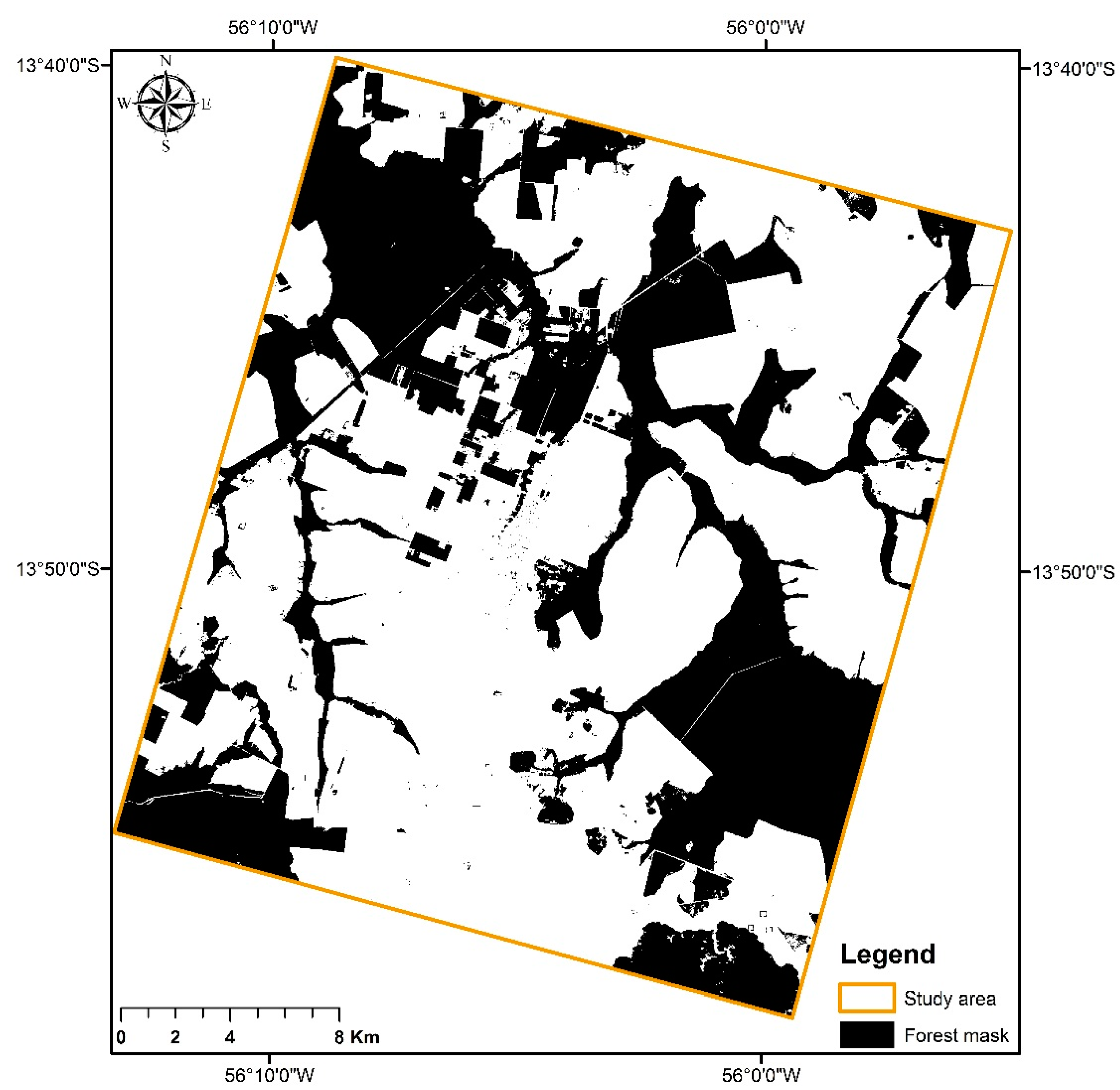
The results showed the importance of integrating satellite images from different sensors to classify the forest and non-forest area. The Program for the Estimation of Amazon Deforestation (PRODES) is the most important project that has been conducting satellite monitoring of deforestation in the Legal Amazon, producing annual deforestation rates in the region, using Landsat images (30 m spatial resolution). Comparing the data of forest areas from the PRODES project with the results of our work, it is possible to verify a high underestimation in the forest areas, mainly in the classes gallery forest and cerrado denso. The PRODES estimated an area of 12,702 ha of forest, and our work estimated an area of 27,326 ha. This difference can be associated to the different spatial resolution used in PRODES (30 m) and in our study (10 m).
Optical images are largely used to map vegetation types in the Cerrado biome. In our results, S2 classifications showed the highest overall accuracy and kappa values. The application of S2 images to map vegetation types in the Cerrado biome is new. In general, Landsat is the most common sensor used to discriminate vegetation types in the Cerrado. Nascimento and Sano [23] had 85% overall accuracy for mapping vegetation types in this biome. The authors used Landsat 7 ETM+ images to discriminate the Rupestrian Cerrado (Savanna formation) in the Chapada dos Veadeiros National Park in Goias State, which can be difficult due to the spectral confusion with other types of Cerrado vegetation. The optical bands located in the red and NIR wavelengths showed high importance and contribution to the discrimination of vegetation type, as was visible in our results (Table 3 and Table 4). Nascimento and Sano (2010) [23] agree on the importance of VIS and NIR regions for characterizing forest areas, as the vegetation has higher reflectance in this wavelength range and is thus more sensitive. Additionally, the number of optical images in ours and other studies helps the increase of discrimination power of different vegetation types, due to the unique spectral signatures of the plant during the year [64,65]. The optical data are certainly useful to map the vegetation type in Cerrado; however, these images are usually not available during the rainy season and the optical data cannot extract information from the structure of the forest [66]. Moreover, the availability of images in the rainy season would allow for a higher temporal resolution, which is crucial to better discriminate the vegetation types in the Cerrado biome due its high seasonality. Additionally, in dense areas of vegetation, the optical sensor is usually saturated due to the low optical depth penetration through these areas, affecting the mapping of the various vegetation types. There are important projects assessing the land use of the Cerrado biome, such as the TerraClass Cerrado project, which produced a map of the land use of the Cerrado biome. However, the project had great difficulties to discriminate the different types of vegetation, which is important for the preservation of biodiversity in this region. Nevertheless, TerraClass presents another step in the challenge of mapping the different types of vegetation in the Cerrado [29].
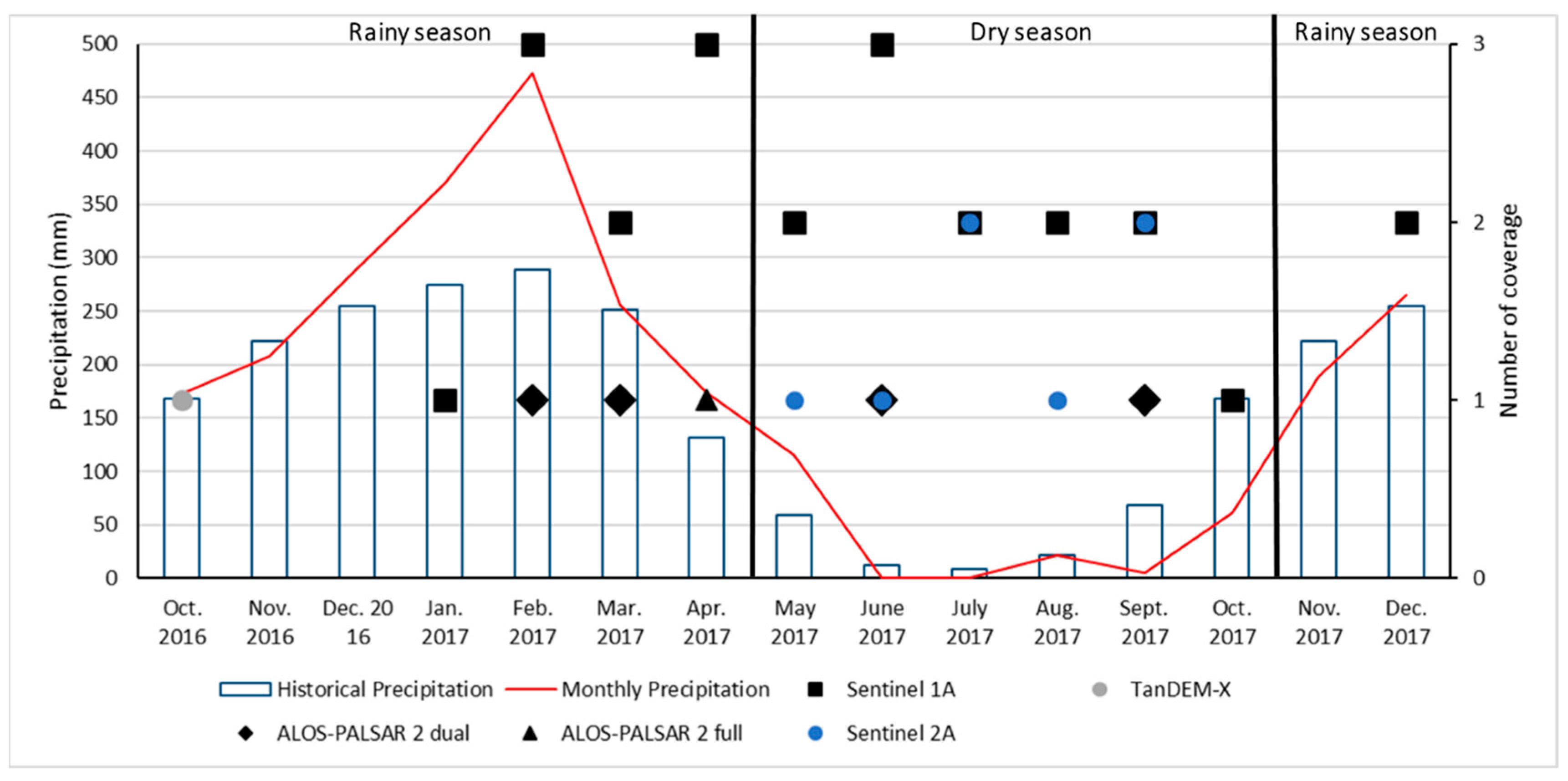
The use of radar images can be a solution to overcome the lack of image availability in the rainy season and the high saturation of optical images in areas of great biomass density. In our radar, classification results from the dry and rainy seasons, TanDEM-X (X Band) and ALOS-PALSAR 2 (L Band) dual polarimetric classification from the dry season showed the highest overall accuracy and kappa values. The influence of vegetation scattering mechanism dependencies is strongly dependent on the wavelength and polarization of the sensor. In the short/intermediate wavelengths, such as X and C Bands, backscattering represents the radiation interaction of canopy, leaves, branches, secondary branches, and part of volumetric scattering (inside crown). Longer wavelengths, such as the L and P Bands, have the capability for deeper penetration. Bigger vegetation components such as trunks, crown, ground, and branches interact with these lower wavelengths. According to the results for the dry season, L Band dual polarimetric images had the highest overall accuracy and kappa values were comparable to the classifications that used single sensor (X and C Bands). The study area is mostly forested. In these areas, radar signals are more likely to be saturated in the X and C Bands compared to the L Bands [67]. The polarization controls the types of components that interact with the radiation. In our study, the L Band cross-polarized HV polarization was the most important variable that contributed to the random classifier in the best classification. This agrees with the fact that cross-polarized images have direct relation with volumetric scattering, and are therefore sensitive to forest structure [68]. There are few studies in the Cerrado biome using only radar images. Sano et al. [34] used the L Band from JERS-1 SAR data to map the different types of vegetation by analyzing the backscattering coefficient values. The study could well separate the grassland, mixed grass/shrub/woodland, and woodland in the state of Distrito Federal.
The results of the CI 95% OAA showed the importance of the fusion between optical and radar data to map vegetation type in the Cerrado biome, since the confidence interval with the narrowest range belonged to the classification that used all images from the dry and rainy seasons, where the narrower the interval, the more accurate the classification. The Cerrado vegetation has one of the largest forest diversities, consequently the combination of different sensors (optical and radar) and spatial resolution (low, medium, and high) results in a great improvement in the accuracy [32]. Of the three classifications that obtained the highest values of accuracy and kappa, two used radar and optical images. This showed the importance of the integration of different sensors in improving the mapping of forest types in Cerrado. A similar result was reported by Sano et al. [38], who combined optical and radar images to improve the classification of different vegetation types in the Cerrado biome. The study had a high overall classification accuracy, which used both sensors in regions of savanna and grasslands formations. Sano et al. [38] used data from the dry and rainy seasons and showed the importance of the time series in improving the classification of different types of vegetation. Additionally, Sano et al. [38] showed better performance of radar data (JERS-1 SAR) compared to optical data (Landsat). In contrast, our results showed that optical data performed better for classification, compared to the radar data. However, this study used a higher number of radar images using L Band compared to our study, which increased the efficiency of mapping vegetation, due to the sensitivity to identify the various structures of the forest, consequently better distinguishing the type of forest, as reported by Lucas et al. [69], Garestier [70], and Santoro [71]. Carvalho et al. [37] used images from ALOS-PALSAR and Landsat to map the different types of vegetation and the results agree on our findings. The highest overall accuracy and kappa values were from the S2 classification; therefore, in our results, the use of radar images did not reach the highest accuracy and kappa values. Carvalho et al. [37] showed that the use of radar data did not improve classification accuracy; however, the study used only one data from radar imaging. Concerning GLCM textures, the same study showed similar results. Grey Level Co-occurrence Matrix textures images had a high variable importance during the Random Forest classification, in particular for entropy, which showed the disorder of GLCM elements. This may be related to the differences in the backscattering of the vegetation type classes.
Regarding the user’s accuracy, the secondary forest was better classified using optical images, whereas the other three classes were better classified using optical and radar images. The optical bands were the most important variables for the RF classifier. The texture images were the second most important ones. Several authors presented similar results achieved in this study [62,72,73]. All mentioned studies showed an improvement in the separability of land cover types employing texture images. The coherence image from TanDEM-X was the third most important variable. Schlund et al. [72] and Baron and Erasmi [62] showed an improvement in the discrimination of forest against other classes using coherence as well.
Other studies about classification of vegetation type in the Cerrado biome, such as Mesquita et al. [35], were in regions where the vegetation has a smaller gradient compared to regions within the Arc of Deforestation, such as Distrito Federal, Minas Gerais, and São Paulo. The IBGE and the MMA mapped vegetation types from the whole Cerrado biome. The studies used Landsat images from the year 2004 and scaling of 1:250,000, which is not enough to detect the gradients of the Cerrado biome. The mapping of vegetation types in transition zones is still a challenge, due to these not having a clear border [74]. However, these regions play an important role in the conservation of the Amazon and Cerrado biome, wherein 75% of the deforestation in Amazon occurs.

5. Conclusions

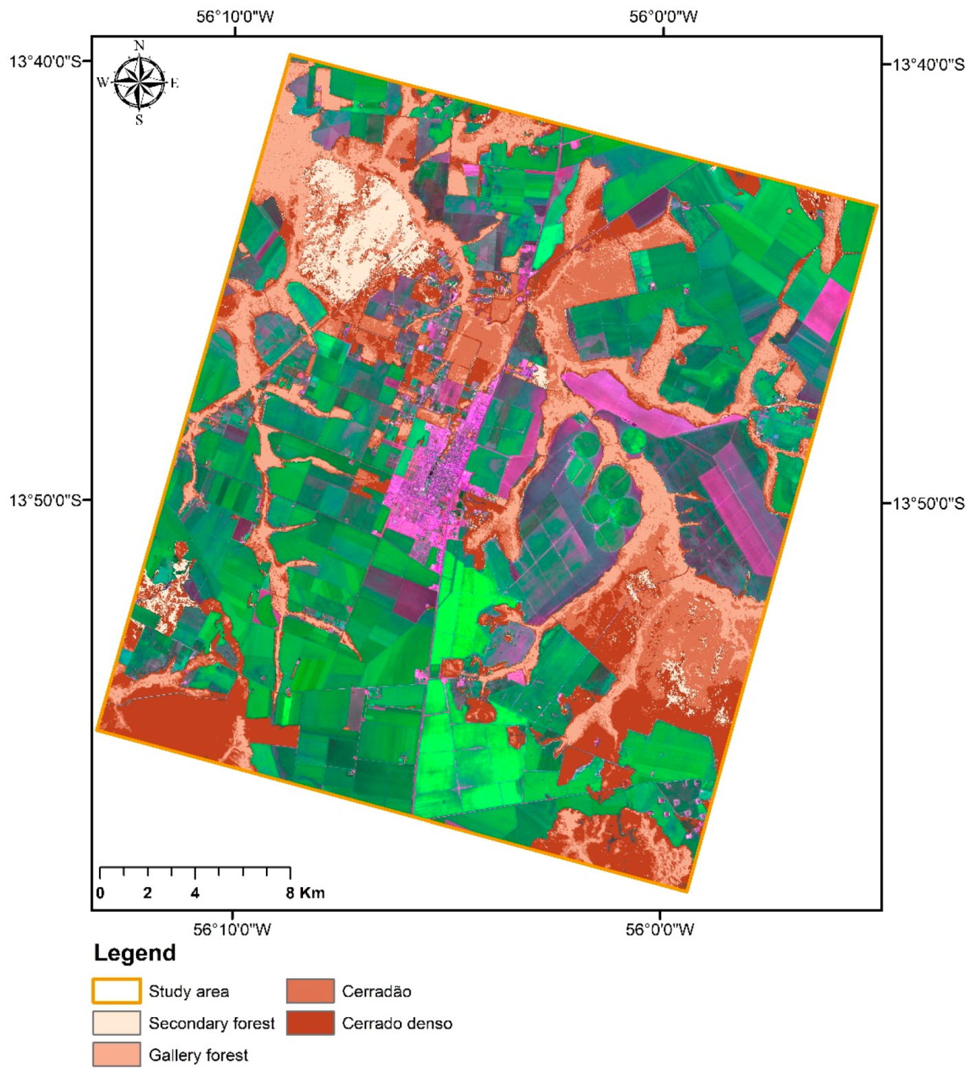
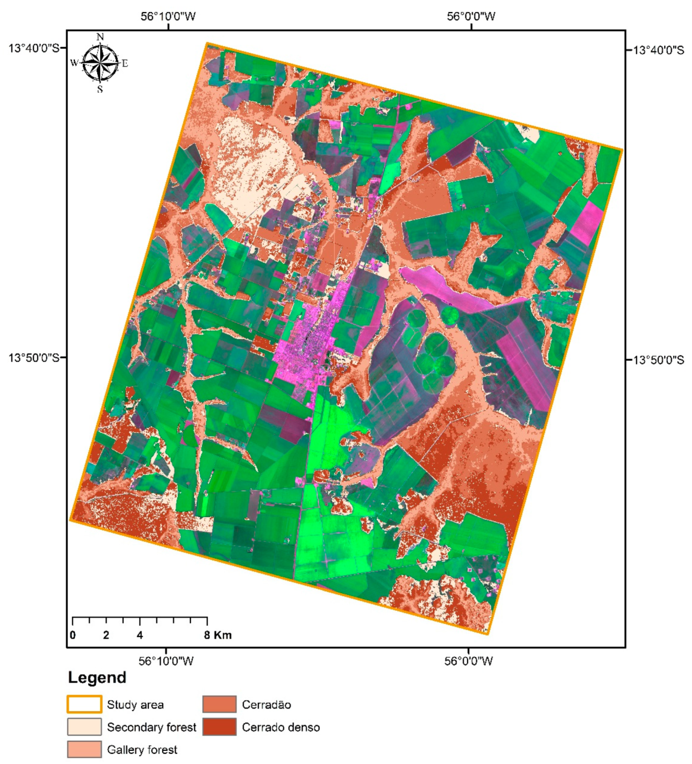
In this paper, we evaluated the use of optical and radar remote sensing for mapping different types of vegetation in the transitional area between the Cerrado and Amazon biomes. The method described in this study improved the mapping of vegetation type in the Arc of Deforestation in the Cerrado biome and can be applied to create accurate vegetation type maps. We evaluated the use of four different sensors, one optical sensor (Sentinel 2) and three radar sensors (Sentinel 1, ALOS, TanDEM-X), for better vegetation type identification and area discrimination, so that these can be used for better calculations of biomass loss and carbon storage in the high dynamic Arc of Deforestation in Brazil.
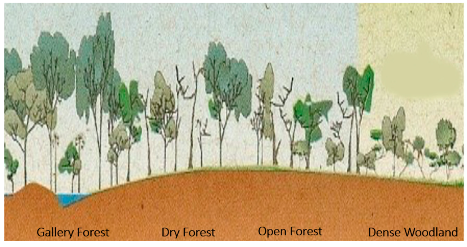
When applying a supervised random forest classification, the highest overall accuracy and kappa coefficient were obtained using only the Sentinel 2A for classification. However, of the three classifications that obtained the highest overall accuracy and kappa values, two used radar and optical images. Bands 5, 11, and 12 of Sentinel 2A, texture images from Sentinel 1A cross-polarization, and coherence of TanDEM-X were the most important images in order to separate each class, as calculated by the random forest variable importance. The combination of optical and radar sensor data usually improves the vegetation classification. Nevertheless, in our study, the single use of optical sensors was sufficient to discriminate the four forest classes in the study area: cerradão (Open Forest), cerrado denso (Dense Woodland), gallery forest, and secondary forest classes in a highly fragmented complex vegetation biome. Such information is relevant for the upcoming mapping of vegetation types in the endangered Cerrado/Amazon ecotone.

Author Contributions

Conceptualization, F.d.S.M., G.G. and S.E.; methodology, F.d.S.M. and S.E.; validation, F.d.S.M., S.E. and G.G.; formal analysis, F.d.S.M. and D.B.; investigation, F.d.S.M.; writing—original draft preparation, F.d.S.M.; writing—review and editing, F.d.S.M., D.B., G.G., V.L. and S.E.; visualization, F.d.S.M., D.B., G.G., V.L. and S.E.

Funding

This research was conducted during a scholarship financed by CAPES—Brazilian Federal Agency for Support and Evaluation of Graduate Education within the Ministry of Education of Brazil (99999.001387/2015-04). The funding of fieldwork was provided from Geo-Gender-Chancenfonds, and Georg-August University School of Science (GAUSS). V.L. was supported by FAPESC (2017TR1762) and CNPq (436863/2018-9; 313887/2018-7).

Acknowledgments

The authors would like to thank the Earth Observation Center (DLR) for providing TanDEM-X data. The Japan Aerospace Exploration Agency (JAXA) for providing ALOS/PALSAR-data, which were obtained under the 4th ALOS Research Announcement (RA, Process 1090), the European Space Agency (ESA) for providing free access to Sentinel 1A and Sentinel 2A data, and the Instituto Nacional de Meteorologia (INMET) for proving free access to precipitation data.

Conflicts of Interest

The authors declare no conflict of interest. The funders had no role in the design of the study; in the collection, analyses, or interpretation of data; in the writing of the manuscript, or in the decision to publish the results.

References

  1. Myers, N.; Mittermeier, R.A.; Mittermeier, C.G.; da Fonseca, G.A.; Kent, J. Biodiversity hotspots for conservation priorities. Nature 2000, 403, 853. [Google Scholar] [CrossRef]
  2. Klink, C.A.; Machado, R.B. A conservação do Cerrado brasileiro. Megadiversidade 2015, 1, 147–155. [Google Scholar]
  3. IBGE. Mapa de Biomas do Brasil, Primeira Aproximação. 2004. Available online: https://ww2.ibge.gov.br/home/presidencia/noticias/21052004biomashtml.shtm (accessed on 10 December 2018).
  4. Castro, A.A.J.F. Comparação florística de espécies do cerrado. Silvicultura 1994, 15, 16–18. [Google Scholar]
  5. EMBRAPA. Sistema Brasileiro de Classificação de Solos; Embrapa: Brasilia, Brazil, 1999. [Google Scholar]
  6. Sano, E.E.; Ferreira, L.G.; Asner, G.P.; Steinke, E.T. Spatial and temporal probabilities of obtaining cloud-free Landsat images over the Brazilian tropical savanna. Int. J. Remote Sens. 2007, 28, 2739–2752. [Google Scholar] [CrossRef]
  7. Walter, B.H. Fitofisionomias do Bioma Cerrado: Síntese Terminológica e Relações Florísticas. Ph.D. Thesis, Universidade de Brasília, Brasília, Brazil, 2006. [Google Scholar]
  8. Fearnside, P.M. Deforestation in Brazilian Amazonia: History, Rates, and Consequences. Conserv. Biol. 2005, 19, 680–688. [Google Scholar] [CrossRef]
  9. Fearnside, P.M.; Righi, C.A.; Graça, P.M.L.D.A.; Keizer, E.W.H.; Cerri, C.C.; Nogueira, E.M.; Barbosa, R.I. Biomass and greenhouse-gas emissions from land-use change in Brazil’s Amazonian “arc of deforestation”: The states of Mato Grosso and Rondônia. For. Ecol. Manag. 2009, 258, 1968–1978. [Google Scholar] [CrossRef]
  10. Felfili, M. Proposição de Critérios Florísticos, Estruturais e de Produção para o Manejo do Cerrado Sensu Stricto do Brasil Central. Ph.D. Thesis, Universidade de Brasília, Brasília, Brazil, 2008. [Google Scholar]
  11. Silva Junior, C.; Aragão, L.; Fonseca, M.; Almeida, C.; Vedovato, L.; Anderson, L. Deforestation-Induced Fragmentation Increases Forest Fire Occurrence in Central Brazilian Amazonia. Forests 2018, 9, 305. [Google Scholar] [CrossRef]
  12. Ramankutty, N.; Foley, J.A.; Olejniczak, N.J. People on the Land: Changes in Global Population and Croplands during the 20th Century. AMBIO J. Hum. Environ. 2002, 31, 251–257. [Google Scholar] [CrossRef]
  13. Machado, R.B.; Ramos Neto, M.B.; Pereira, P.G.P.; Caldas, E.F.; Gonçalves, D.A.; Santos, N.S.; Tabor, K.; Steininger, M. Estimativas de Perda da Área do Cerrado Brasileiro; Relatório técnico; Conservação Internacional: Brasilia, Brazil, 2004. [Google Scholar]
  14. Janssen, T.A.J.; Ametsitsi, G.K.D.; Collins, M.; Adu-Bredu, S.; Oliveras, I.; Mitchard, E.T.A.; Veenendaal, E.M. Extending the baseline of tropical dry forest loss in Ghana (1984–2015) reveals drivers of major deforestation inside a protected area. Biol. Conserv. 2018, 218, 163–172. [Google Scholar] [CrossRef]
  15. Hirota, M.; Nobre, C.; Oyama, M.D.; Bustamante, M.M.C. The climatic sensitivity of the forest, savanna and forest-savanna transition in tropical South America. New Phytol. 2010, 187, 707–719. [Google Scholar] [CrossRef] [Green Version]
  16. Macedo, M.N.; DeFries, R.S.; Morton, D.C.; Stickler, C.M.; Galford, G.L.; Shimabukuro, Y.E. Decoupling of deforestation and soy production in the southern Amazon during the late 2000s. Proc. Natl. Acad. Sci. USA 2012, 109, 1341–1346. [Google Scholar] [CrossRef] [Green Version]
  17. INPE. Program for the Estimation of Amazon Deforestation (PRODES). 2011. Available online: http://www.dpi.inpe.br/prodesdigital/prodesmunicipal.php (accessed on 15 January 2019).
  18. Soares-Filho, B.; Rajão, R.; Macedo, M.; Carneiro, A.; Costa, W.; Coe, M.; Rodrigues, H.; Alencar, A. Land use. Cracking Brazil’s Forest Code. Science 2014, 344, 363–364. [Google Scholar] [CrossRef] [PubMed]
  19. Marques, E.Q.; Marimon-Junior, B.H.; Marimon, B.S.; Matricardi, E.A.T.; Mews, H.A.; Colli, G.R. Redefining the Cerrado–Amazonia transition: Implications for conservation. Biodivers. Conserv. 2019, 1–17. [Google Scholar] [CrossRef]
  20. Nogueira, E.M.; Fearnside, P.M.; Nelson, B.W.; França, M.B. Wood density in forests of Brazil’s ‘arc of deforestation’: Implications for biomass and flux of carbon from land-use change in Amazonia. For. Ecol. Manag. 2007, 248, 119–135. [Google Scholar] [CrossRef]
  21. Bitencourt, M.D.; de Mesquita, H.N., Jr.; Mantovani, W.; Batalha, M.A.; Pivello, V.R. Identificação de fisionomias de cerrado com imagem índice de vegetação. In Contribuição ao Conhecimento Ecológico do Cerrado; Editora Universidade de Brasília: Brasilia, Brazil, 1997; pp. 316–320. [Google Scholar]
  22. Liesenberg, V.; Galvão, L.S.; Ponzoni, F.J. Variations in reflectance with seasonality and viewing geometry: Implications for classification of Brazilian savanna physiognomies with MISR/Terra data. Remote Sens. Environ. 2007, 107, 276–286. [Google Scholar] [CrossRef]
  23. Nascimento, E.R.P.; Sano, E.E. Identificação de Cerrado Rupestre por Meio de Imagens Multitemporais do Landsat: Proposta Metodológica. Soc. Nat. 2010, 22, 93–106. [Google Scholar] [CrossRef]
  24. Ferreira, M.E.; Ferreira, L.G.; Sano, E.E.; Shimabukuro, Y.E. Spectral linear mixture modelling approaches for land cover mapping of tropical savanna areas in Brazil. Int. J. Remote Sens. 2007, 28, 413–429. [Google Scholar] [CrossRef]
  25. Girolamo Neto, C.D.; Fonseca, L.M.G.; Körting, T.S. Assessment of texture features for Brazilian savanna classification: A case study in Brasília national park. Braz. J. Cartogr. 2017, 69, 891–901. [Google Scholar]
  26. Schwieder, M.; Leitão, P.J.; da Cunha Bustamante, M.M.; Ferreira, L.G.; Rabe, A.; Hostert, P. Mapping Brazilian savanna vegetation gradients with Landsat time series. Int. J. Appl. Earth Observ. Geoinf. 2016, 52, 361–370. [Google Scholar] [CrossRef]
  27. Müller, H.; Rufin, P.; Griffiths, P.; Barros Siqueira, A.J.; Hostert, P. Mining dense Landsat time series for separating cropland and pasture in a heterogeneous Brazilian savanna landscape. Remote Sens. Environ. 2015, 156, 490–499. [Google Scholar] [CrossRef] [Green Version]
  28. Sano, E.E.; Rosa, R.; Brito, J.L.S.; Ferreira, L.G. Land cover mapping of the tropical savanna region in Brazil. Environ. Monit. Assess. 2010, 166, 113–124. [Google Scholar] [CrossRef]
  29. MMA. Mapeamento do Uso e Cobertura da Terra do Cerrado. Projeto TerraClass Cerrado 2013; Brasília. 2015. Available online: http://www.mma.gov.br/images/arquivo/80049/Cerrado/publicacoes/Livro%20EMBRAPA-WEB-1-TerraClass%20Cerrado.pdf (accessed on 20 November 2018).
  30. Almeida-Filho, R.; Shimabukuro, Y.E. Detecting areas disturbed by gold mining activities through JERS-1 SAR images, Roraima State, Brazilian Amazon. Int. J. Remote Sens. 2010, 21, 3357–3362. [Google Scholar] [CrossRef]
  31. Evans, T.L.; Costa, M. Landcover classification of the Lower Nhecolândia subregion of the Brazilian Pantanal Wetlands using ALOS/PALSAR, RADARSAT-2 and ENVISAT/ASAR imagery. Remote Sens. Environ. 2013, 128, 118–137. [Google Scholar] [CrossRef]
  32. Saatchi, S.S.; Nelson, B.; Podest, E.; Holt, J. Mapping land cover types in the Amazon Basin using 1 km JERS-1 mosaic. Int. J. Remote Sens. 2010, 21, 1201–1234. [Google Scholar] [CrossRef]
  33. Santos, J.R.; Xaud, M.R.; Pardi Lacruz, M.S. Analysis of the backscattering signals of JERS-1 image from savanna and tropical rainforest biomass in Brazilian Amazonia. In Proceedings of the International Symposium on Resource and Environmental Monitoring, Budapest, Hungary, 1–4 September 1998. [Google Scholar]
  34. Sano, E.E.; Pinheiro, G.C.C.; Meneses, P.R. Assessing JERS-1 synthetic aperture radar data for vegetation mapping in the Brazilian savanna. J. Remote Sens. Soc. Jpn. 2001, 21, 158–167. [Google Scholar]
  35. Mesquita JR, H.N.; Bittencourt, M.D.; Kuntschik, G. Gradient analysis of cerrado vegetation physiognomies by SAR image processing (JERS-1). In Proceedings of the X Simpósio Brasileiro de Sensoriamento Remoto, Foz do Iguacú, Brasil, 21–26 Abril 2001. [Google Scholar]
  36. Bitencourt, M.D.; de Mesquita, J.H.N.; Kuntschik, G.; da Rocha, H.R.; Furley, P.A. Cerrado vegetation study using optical and radar remote sensing: Two Brazilian case studies. Can. J. Remote Sens. 2007, 33, 468–480. [Google Scholar] [CrossRef]
  37. Carvalho, L.; Rahman, M.; Hay, G.; Yackel, J. Optical and SAR imagery for mapping vegetation gradientsin Brazilian savannas: Synergy between pixel-based andobject-based approaches. In Proceedings of the International Conference of Geographic Object-Based Image, Ghent, Belgium, 29 June–2 July 2010. [Google Scholar]
  38. Sano, E.E.; Ferreira, L.G.; Huete, A.R. Synthetic Aperture Radar (L band) and Optical Vegetation Indices for Discriminating the Brazilian Savanna Physiognomies: A Comparative Analysis. Earth Interact. 2005, 9, 1–15. [Google Scholar] [CrossRef]
  39. Zaiatz, A.P.S.R.; Zolin, C.A.; Vendrusculo, L.G.; Lopes, T.R.; Paulino, J. Agricultural land use and cover change in the Cerrado/Amazon ecotone: A case study of the upper Teles Pires River basin. Acta Amaz. 2018, 48, 168–177. [Google Scholar] [CrossRef] [Green Version]
  40. Goedert, W.J. Solos dos Cerrados. Tecnologias e Estratégias de Manejo; EMBRAPA, Centro de Pesquisa Agropecuária dos Cerrados; Nobel: Brasília, Brasil, 1986. [Google Scholar]
  41. IBGE. Mapa de Solos do Brasil. 2001. Available online: ftp://geoftp.ibge.gov.br/informacoes_ambientais/pedologia/mapas/brasil/solos.pdf (accessed on 11 November 2018).
  42. Rudorff, B.F.T.; Adami, M.; Risso, J.; de Aguiar, D.A.; Pires, B.; Amaral, D.; Fabiani, L.; Cecarelli, I. Remote Sensing Images to Detect Soy Plantations in the Amazon Biome—The Soy Moratorium Initiative. Sustainability 2012, 4, 1074–1088. [Google Scholar] [CrossRef] [Green Version]
  43. Ribeiro, J.F.; Walter, B.M.T. As principais fitofisionomias do Bioma Cerrado. In Cerrado: Ecologia e Flora; Sano, S.M., Almeida, S.P., Ribeiro, J.F., Eds.; Embrapa Cerrados: Brasília, Brazil, 2008; pp. 151–212. [Google Scholar]
  44. Ferreira, R.L.C. Estrutura e Dinâmica de uma Floresta Secundária de Transição, Rio Vermelho e Serra Azul de Minas, MG. Ph.D. Thesis, Universidade Federal de Viçosa, Viçosa, Brasil, 1997. [Google Scholar]
  45. Louis, J.; Debaecker, V.; Pflug, B.; Main-Knorn, M.; Bieniarz, J.; Mueller-Wilm, U.; Cadau, E.; Gascon, F. Sentinel-2 Sen2Cor: L2A Processor for Users. In Proceedings of the ESA Living Planet Symposium 2016, Prague, Czech Republic, 9–13 May 2016. [Google Scholar]
  46. Sabins, F.F. Remote sensing for mineral exploration. Ore Geol. Rev. 1999, 14, 157–183. [Google Scholar] [CrossRef]
  47. Rosich, B.; Meadows, P. Absolute Calibration of ASAR Level 1 Products Generated with PF-ASAR. 2004. Available online: https://earth.esa.int/web/guest/-/absolute-calibration-of-asar-level-1-products-generated-with-pf-asar-4503 (accessed on 10 August 2018).
  48. Small, D. Flattening Gamma: Radiometric Terrain Correction for SAR Imagery. IEEE Trans. Geosci. Remote Sens. 2011, 49, 3081–3093. [Google Scholar] [CrossRef]
  49. Yague-Martinez, N.; Zan, F.D.; Prats-Iraola, P. Coregistration of Interferometric Stacks of Sentinel-1 TOPS Data. IEEE Geosci. Remote Sens. Lett. 2017, 14, 1002–1006. [Google Scholar] [CrossRef]
  50. Haralick, R.M.; Shanmugam, K.; Dinstein, I.H. Textural Features for Image Classification. IEEE Trans. Syst. Man Cybern. 1973, SMC-3, 610–621. [Google Scholar] [CrossRef]
  51. Lee, J.-S.; Pottier, E. (Eds.) Polarimetric Radar Imaging. From Basics to Applications; CRC: London, UK; Taylor & Francis [Distributor]: Boca Raton, FL, USA, 2009; ISBN 142005497X. [Google Scholar]
  52. Schreier, G. SAR Geocoding. Data and Systems; Wichmann: Karlsruhe, Germany, 1993; ISBN 3879072477. [Google Scholar]
  53. Pottier, E.; Lee, J.; Ferro-Famil, L. PolSARPro_v4.2.0-Tutorial-Part1 Radar Polarimetry-4 Polarimetric Decompositions. 2007. [Google Scholar]
  54. Pereira, L.; Furtado, L.; Novo, E.; Sant’Anna, S.; Liesenberg, V.; Silva, T. Multifrequency and Full-Polarimetric SAR Assessment for Estimating Above Ground Biomass and Leaf Area Index in the Amazon Várzea Wetlands. Remote Sens. 2018, 10, 1355. [Google Scholar] [CrossRef]
  55. Cloude, S.R.; Pottier, E. A review of target decomposition theorems in radar polarimetry. IEEE Trans. Geosci. Remote Sens. 1996, 34, 498–518. [Google Scholar] [CrossRef]
  56. Furtado, L.F.D.A.; Silva, T.S.F.; Novo, E.M.L.D.M. Dual-season and full-polarimetric C band SAR assessment for vegetation mapping in the Amazon várzea wetlands. Remote Sens. Environ. 2016, 174, 212–222. [Google Scholar] [CrossRef]
  57. Krieger, G.; Moreira, A.; Fiedler, H.; Hajnsek, I.; Werner, M.; Younis, M.; Zink, M. TanDEM-X: A Satellite Formation for High-Resolution SAR Interferometry. IEEE Trans. Geosci. Remote Sens. 2007, 45, 3317–3341. [Google Scholar] [CrossRef] [Green Version]
  58. Bamler, R.; Hartl, P. Synthetic aperture radar interferometry. Inverse Probl. 1998, 14, R1. [Google Scholar] [CrossRef]
  59. Breiman, L. Random Forests. Mach. Learn. 2001, 45, 5–32. [Google Scholar] [CrossRef] [Green Version]
  60. Bradter, U.; Thom, T.J.; Altringham, J.D.; Kunin, W.E.; Benton, T.G. Prediction of National Vegetation Classification communities in the British uplands using environmental data at multiple spatial scales, aerial images and the classifier random forest. J. Appl. Ecol. 2011, 48, 1057–1065. [Google Scholar] [CrossRef] [Green Version]
  61. Baron, D.; Erasmi, S. High Resolution Forest Maps from Interferometric TanDEM-X and Multitemporal Sentinel-1 SAR Data. PFG J. Photogramm. Remote Sens. Geoinf. Sci. 2017, 85, 389–405. [Google Scholar] [CrossRef]
  62. Congalton, R.G. A review of assessing the accuracy of classifications of remotely sensed data. Remote Sens. Environ. 1991, 37, 35–46. [Google Scholar] [CrossRef]
  63. Olofsson, P.; Foody, G.M.; Herold, M.; Stehman, S.V.; Woodcock, C.E.; Wulder, M.A. Good practices for estimating area and assessing accuracy of land change. Remote Sens. Environ. 2014, 148, 42–57. [Google Scholar] [CrossRef] [Green Version]
  64. Hermuche, P.M.; Sano, E.E. Identificação da floresta estacional decidual no Vão do Paraná, estado de Goiás, a partir da analise da reflectância acumulada de imagens do sensor ETM+/Landsat-7. Revista Brasileira de Cartografia 2011, 63, 415–425. [Google Scholar]
  65. Barret, B.; Raab, C.; Cawkwell, F.; Grenn, S. Upland vegetation mapping using Random Forests with optical and radar satellite data. Remote Sens. Ecol. Conserv. 2016, 2, 212–231. [Google Scholar] [CrossRef] [Green Version]
  66. Asner, G.P. Cloud cover in Landsat observations of the Brazilian Amazon. Int. J. Remote Sens. 2001, 3855–3862. [Google Scholar] [CrossRef]
  67. Yu, Y.; Saatchi, S. Sensitivity of L-Band SAR Backscatter to Aboveground Biomass of Global Forests. Remote Sens. 2016, 8, 522. [Google Scholar] [CrossRef]
  68. Jensen, J.R. Remote Sensing of the Environment. An Earth Resource Perspective, 2nd ed.; Pearson Prentice Hall: Upper Saddle River, NJ, USA, 2007; ISBN 0131889508. [Google Scholar]
  69. Lucas, R.M.; Milne, A.K.; Cronin, N.; Witte, C.; Denham, R. The potential of synthetic aperture radar (SAR) for quantifying the biomass of Australia’s woodlands. Rangel. J. 2000, 22, 124–140. [Google Scholar] [CrossRef]
  70. Garestier, F.; Dubois-Fernandez, P.C.; Guyon, D.; Le Toan, T. Forest Biophysical Parameter Estimation Using L- and P-Band Polarimetric SAR Data. IEEE Trans. Geosci. Remote Sens. 2009, 47, 3379–3388. [Google Scholar] [CrossRef]
  71. Santoro, M.; Fransson, J.E.S.; Eriksson, L.E.B.; Magnusson, M.; Ulander, L.M.H.; Olsson, H. Signatures of ALOS PALSAR L-Band Backscatter in Swedish Forest. IEEE Trans. Geosci. Remote Sens. 2009, 47, 4001–4019. [Google Scholar] [CrossRef] [Green Version]
  72. Schlund, M.; von Poncet, F.; Hoekman, D.H.; Kuntz, S.; Schmullius, C. Importance of bistatic SAR features from TanDEM-X for forest mapping and monitoring. Remote Sens. Environ. 2014, 151, 16–26. [Google Scholar] [CrossRef]
  73. Inglada, J.; Vincent, A.; Arias, M.; Marais-Sicre, C. Improved Early Crop Type Identification By Joint Use of High Temporal Resolution SAR And Optical Image Time Series. Remote Sens. 2016, 8, 362. [Google Scholar] [CrossRef]
  74. Ribeiro, J.F.; Walter, B.M.T. Fitofisionomias do Bioma Cerrado. 1998. Available online: http://www.bdpa.cnptia.embrapa.br/consulta/busca?b=ad&id=554094&biblioteca=vazio&busca=554094&qFacets=554094&sort=&paginacao=t&paginaAtual=1 (accessed on 10 August 2018).
Figure 1. Location of the study area within the South America context. The scene footprint of different satellites are shown on top of a Google Earth image.
Remotesensing 11 01161 g001
Figure 2. Cerrado biome phytophysiognomies. The graphic depicts two vegetation formations and their subdivisions in the study area, except the Dry Forest. Source: Adapted from [43].
Remotesensing 11 01161 g002
Figure 3. . Historical (1961–2017) and Monthly (2016–2017) precipitation values and acquisition dates of Sentinel 2A, ALOS PALSAR 2 full, ALOS PALSAR 2 dual, TanDEM-X and Sentinel 1A. Precipitation data were collected from the Diamatino fluviometric station located near to the study area.
Remotesensing 11 01161 g003
Figure 4. Flowchart of the proposal methodology.
Remotesensing 11 01161 g004
Figure 5. Distribution of Random Forest and non-forest samples and forest type samples (4 classes) in the study area, on top of a false color composition of Sentinel 2A Band 3, 4, and 8 (07 July 2017).
Remotesensing 11 01161 g005
Figure 6. Forest mask extracted from the classification of Sentinel 2A with ALOS-PALSAR full polarimetric PC1 images.
Remotesensing 11 01161 g006
Figure 7. Classification results of the spatial distribution of the four Cerrado forest types using Sentinel 2A (dry season) on top of a false color composition of Sentinel 2A, Bands 3, 4, and 8 (07 July 2017).
Remotesensing 11 01161 g007
Figure 8. Producer’s (A) and user’s (B) accuracy of classifications based on single-sensor and optical/SAR-combinations for the four Cerrado types. Only data acquisitions during the dry season were considered.
Remotesensing 11 01161 g008
Figure 9. Classification of Cerrado forest type using all images from the dry and rainy season on top of a false color composition from Sentinel 2A, Bands 3, 4, and 8 (07 July 2017).
Remotesensing 11 01161 g009
Figure 10. Producer’s (A) and user’s (B) accuracy of classifications based on single-sensor and optical/SAR-combinations for the four Cerrado types. All data acquisitions during the dry and rainy season were considered.
Remotesensing 11 01161 g010
Table 1. Characteristics of the selected satellite images and the accumulated precipitation values three days before Radar acquisition.
SensorDatePolarizationOrbitAccumulated Precipitation Values 3 Days Before Radar Acquisition (mm)
Sentinel 1A08.01.2017Dual—VH and VVDescending3.3
01.02.201711.5
13.02.201758.3
25.02.201730.2
09.03.201727.2
21.03.201724.0
02.04.201716.8
14.04.20170
26.04.201733.3
08.05.20170
20.05.20170
01.06.20170
13.06.20170
25.06.20170
19.07.20170
31.07.20170
12.08.20170
24.08.20170
05.09.20170
17.09.20170
11.10.20170
10.12.201788.7
22.12.20170
TanDEM-X20.10.2016Single—HH 8.1
ALOS-PALSAR 2 dual01.02.2017Dual—HH and HVAscending11.5
26.03.2017Descending35.7
04.06.20170
13.09.2017Ascending0
ALOS-PALSAR 2 full13.04.2017FullAscending0
27.04.20170
Sentinel 2A07.05.2017--0
16.06.20170
06.07.20170
26.07.20170
15.08.201719.2
04.09.20170
24.09.20170
Table 2. Classification scheme (number in brackets shows the number of variables per input data set).
Dry Season (SAR and Optical)Rainy + Dry Seasons (SAR and Optical)Dry Season (SAR)Rainy + Dry Seasons (SAR)
Sentinel 2A (10)Sentinel 1A (44)Sentinel 1A + TanDEM-XSentinel 1A + TanDEM-X
Sentinel 1A (22)ALOS2 full (6)Sentinel 1A + ALOS2 dualSentinel 1A + ALOS2 dual
TanDEM-X (3)Sentinel 2A + Sentinel 1ASentinel 1A + ALOS2 fullSentinel 1A + ALOS2 full
ALOS2 dual (4)Sentinel 2A + ALOS2 fullTanDEM-X + ALOS2 fullTanDEM-X + ALOS2 full
Sentinel 2A + Sentinel 1AAll imagesALOS2 dual + ALOS2 fullALOS2 dual + ALOS2 full
Sentinel 2A + TanDEM-X
Sentinel 2A + ALOS2 dual
All images
Table 3. Overall accuracy, kappa, confidence interval 95%, overall average accuracy (OAA), and the three most important variables for the classifications based on the Random Forest variable importance for Sentinel 2A (S2), ALOS PALSAR 2 full (A2f), ALOS PALSAR 2 dual (A2d), TanDEM X (TX), and Sentinel 1A (S1). The parameters listed in the variable importance are the PC1 derived from the PCA, except for the images from TanDEM-X, as only one acquisition was available. Only data acquisitions during the dry season were considered.
Dry Season (SAR and Optical)Overall AccuracyKappaConf. 95% OAAVariable
Sentinel 2A82.60%0.772.29Bands 11, 12, 5
Sentinel 1A48.51%0.312.76Entropy VV, mean VV, variance VH
TanDEM-X58.22%0.442.78Coherence, intensity master, intensity slave
ALOS2 dual59.70%0.462.73HH descending, HV descending, HH ascending
Sentinel 2A + Sentinel 1A79.90%0.732.08Bands 12, 11, 5 S2
Sentinel 2A + TanDEM-X81.91%0.762.14Band 11 S2, Band 12 S2, coherence HH TX
Sentinel 2A + ALOS2 dual74.91%0.672.53Band 11 S2, HV descending A2d, HH descending A2d
All images80.33%0.742.05Band 11 S2, HV descending A2d, Band 12 S2
Table 4. Overall accuracy, kappa values, confidence interval 95% OAA, the three most important variables for the classifications according to Random Forest variable importance for Sentinel 2A (S2), ALOS PALSAR 2 full (A2f), ALOS PALSAR 2 dual (A2d), TanDEM X (TX), and Sentinel 1A (S1). The parameters listed in the variable importance are the PC1 derived from the PCA, except for the images from TanDEM-X, as only one acquisition was available. All data acquisitions during the dry and rainy season were considered.
Rainy + Dry SeasonOverall AccuracyKappaConf. 95% OAAVariable Importance
Sentinel 1A56.21%0.422.87Entropy VV, mean VV, contrast VH
ALOS2 full41.26%0.222.77Volumetric, C22, C11
Sentinel 2A + Sentinel 1A81.73%0.762.05Bands 12 S2, 11 S2, contract VH S1 rainy season
Sentinel 2A + ALOS2 full79.98%0.732.28Bands 11, 12, 5 S2
All images81.91%0.761.97Band 11 S2, HV descending A2d, Band 12 S2
Table 5. Overall accuracy, kappa values, confidence interval 95% OAA, and the three most important variables for the classifications based on the Random Forest variable importance for Sentinel 2A (S2), ALOS PALSAR 2 full (A2f), ALOS PALSAR 2 dual (A2d), TanDEM X (TX), and Sentinel 1A (S1). The parameters listed in the variable importance are the PC1 derived from the PCA except for the images from TanDEM-X, as only one acquisition was available.
Dry SeasonOverall AccuracyKappaConf. 95% OAAVariable Importance
Sentinel 1A + TanDEM-X54.46%0.392.66Coherence HH TX, mean VV S1, entropy VV S1
Sentinel 1A + ALOS2 dual62.33%0.502.61HV descending A2d, HH descending A2d, HV ascending A2d
TanDEM-X + ALOS2 dual66.96%0.562.61HV descending A2d, HH descending A2d, coherence HH TX
Rainy + dry season
Sentinel 1A + TanDEM-X64.42%0.530.67Coherence HH TX, mean VV S1 dry season, entropy VV S1 dry season
Sentinel 1A + ALOS2 dual66.61%0.552.69HV descending A2d, HH descending A2d, contrast VH S1 rainy season
Sentinel 1A + ALOS2 full61.10%0.482.78Volumetric, entropy VV S1 dry seanson, mean VV S1 dry season
TanDEM-X + ALOS2 full61.01%0.482.81Coherence HH TX, volumetric A2f, C22 A2f
ALOS2 dual + ALOS2 full58.30%0.442.81HV descending A2d, HH descening A2d, HH ascending A2d
Table 6. Producer’s and user’s accuracy of classifications based only on combinations of SAR sensors for the four Cerrado types. Only data acquisitions during the dry season were considered.
Dry SeasonCerrado DensoCerradãoGallery ForestSecondary Forest
Producer’s accuracy
Sentinel 1A + TanDEM-X40.21%28.52%94.46%54.04%
Sentinel 1A + ALOS2 dual38.11%34.86%76.12%100.00%
TanDEM-X + ALOS2 dual40.91%59.86%67.13%100.00%
User’s accuracy
Sentinel 1A + TanDEM-X50.88%24.92%73.19%70.00%
Sentinel 1A + ALOS2 dual53.96%34.14%70.97%83.33%
TanDEM-X + ALOS2 dual68.02%47.22%72.93%82.37%
Table 7. Producer’s and user’s accuracy of classifications based only on combinations of SAR sensors for the four Cerrado types. All data acquisitions during the dry and rainy seasons were considered.
Rainy + Dry SeasonsCerrado DensoCerradãoGallery ForestSecondary Forest
Producer’s accuracy
Sentinel 1A + TanDEM-X53.85%40.85%94.81%67.72%
Sentinel 1A + ALOS2 dual55.24%44.72%66.44%100.00%
Sentinel 1A + ALOS2 full47.90%36.97%92.04%67.02%
TanDEM-X + ALOS2 full43.36%42.61%78.89%78.95%
ALOS2 dual + ALOS2 full41.96%51.41%40.14%100.00%
User’s accuracy
Sentinel 1A + TanDEM-X71.96%37.54%76.75%73.11%
Sentinel 1A + ALOS2 dual65.29%44.88%76.19%77.66%
Sentinel 1A + ALOS2 full59.57%40.70%68.56%71.27%
TanDEM-X + ALOS2 full56.36%39.41%67.66%80.36%
ALOS2 dual + ALOS2 full45.63%46.79%58.29%77.03%

