Moving Object Detection and Tracking with Doppler LiDAR


Abstract
:
1. Introduction
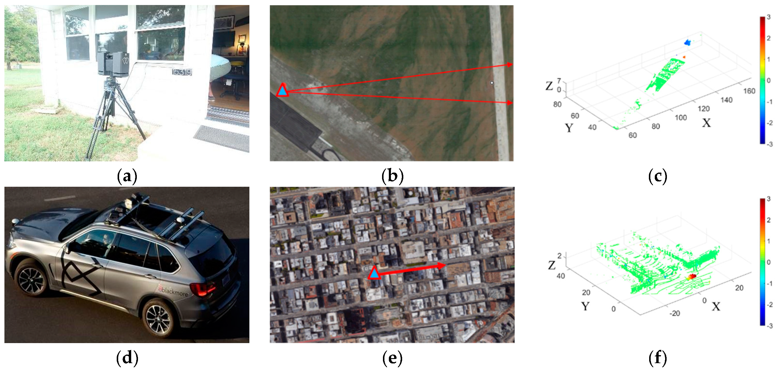
2. Data
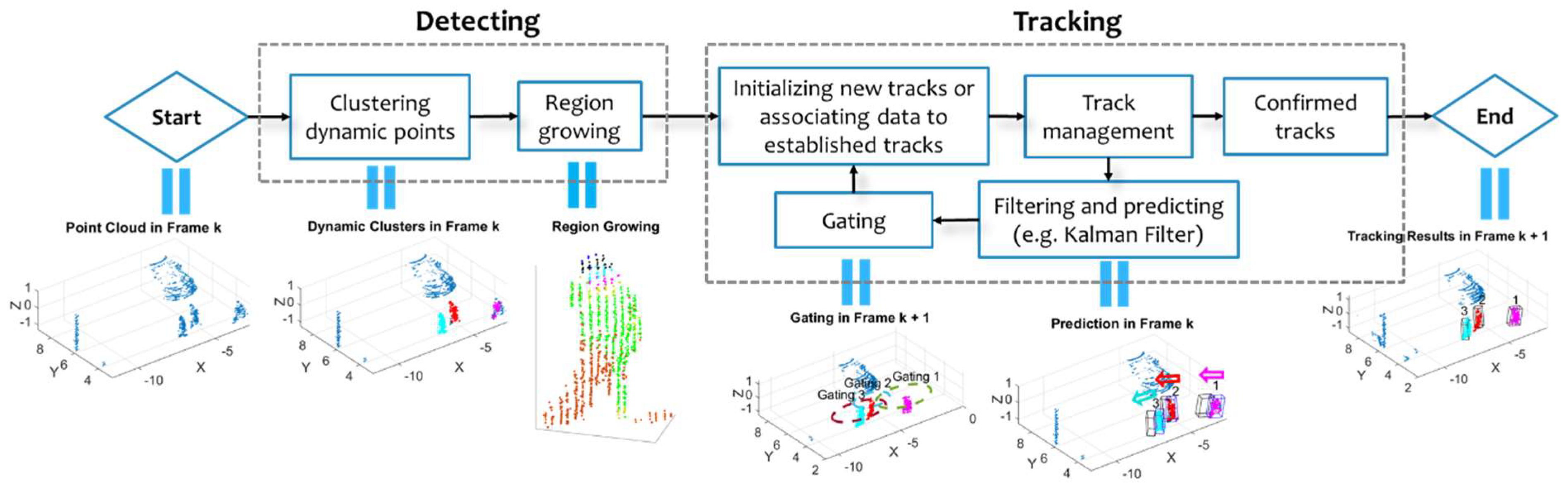
3. Moving Object Detection
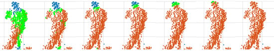
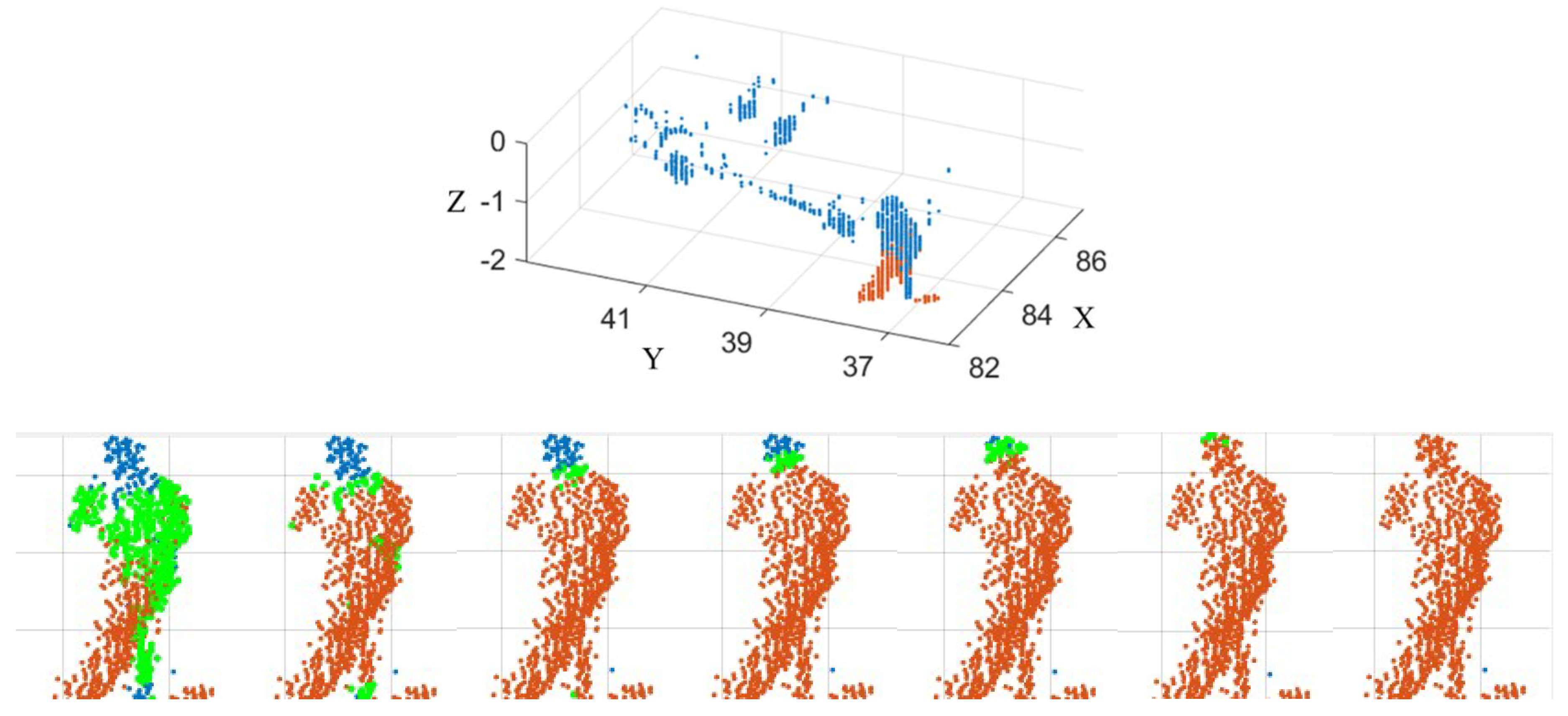
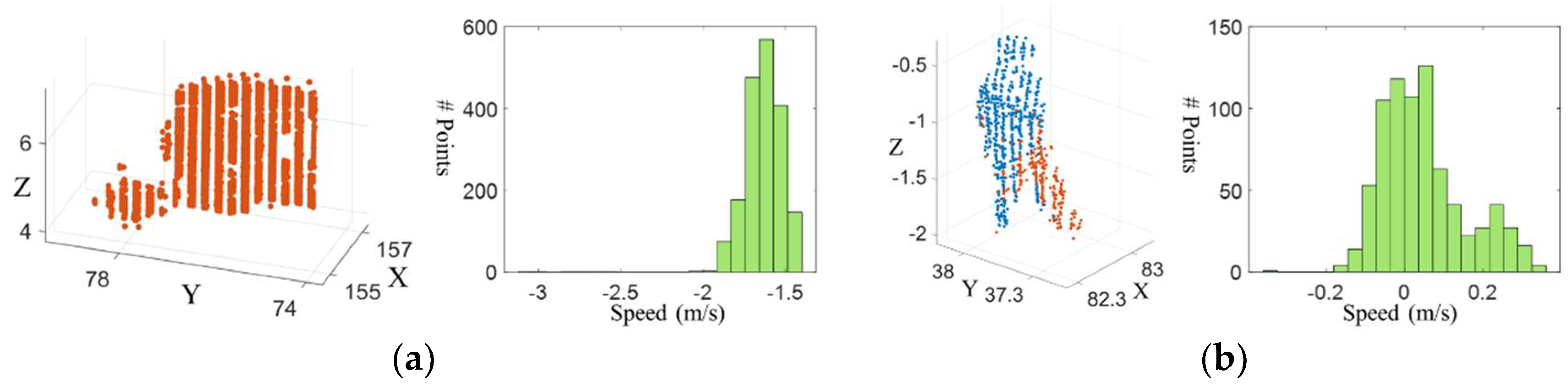
3.1. Moving Points Detection and Clustering
- (1)
- Randomly choose an unvisited point ;
- (2)
- Calculate the adaptive distance threshold with the range and the azimuth sampling resolution ;
- (3)
- Find all the neighboring points within spatial distance and within temporal distance to . If the number of neighboring points is larger than , go to step 4; else, label as the visited noisy point and go back to step 1;
- (4)
- Cluster all points that are density reachable or density connecting [26] to point and label them as visited. Go back to step 2;
- (5)
- Terminate the process after all the points are visited. The output is a set of clusters of dynamic points .
3.2. Clustering Static Points—Completing the Objects
- (1)
- Choose an unvisited dynamic cluster from ;
- (2)
- For each point in , calculate the mean distance from to its K-nearest neighboring points. The mean distance within cluster with M points is calculated as ;
- (3)
- Find all static points in within and from at least one point in ;
- (4)
- If no point is left in , go to step 1; otherwise, merge to cluster and go to step 2;
- (5)
- Terminate the region growing process when all members in are visited.
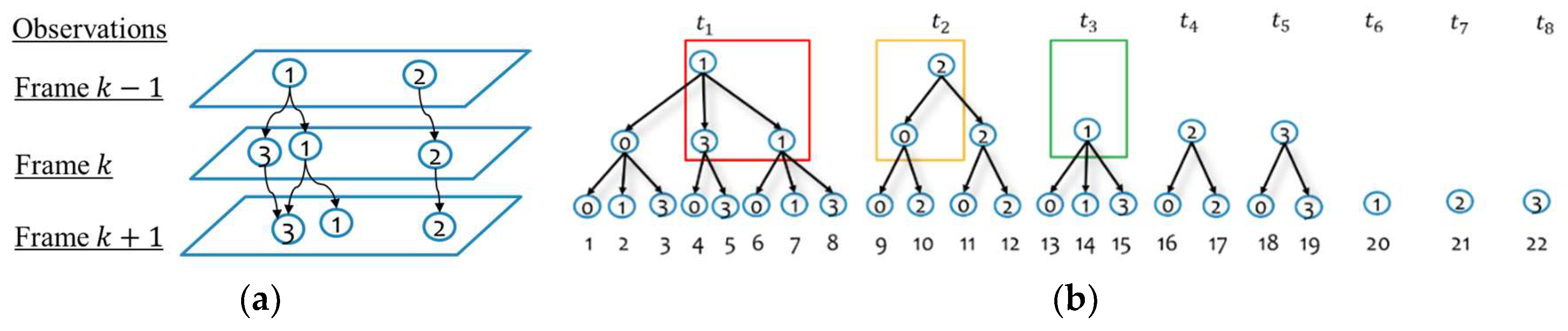
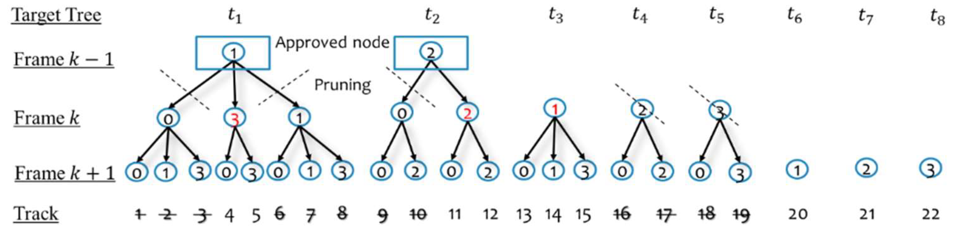
4. Moving Object Tracking
4.1. Kalman Filter with Doppler Images
4.2. Gating and Proposing Track Hypotheses
4.3. Scoring
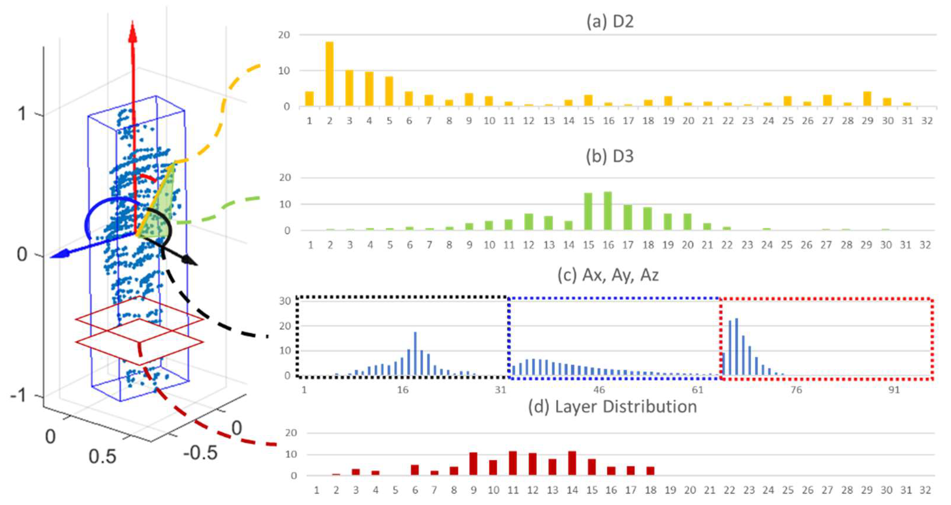
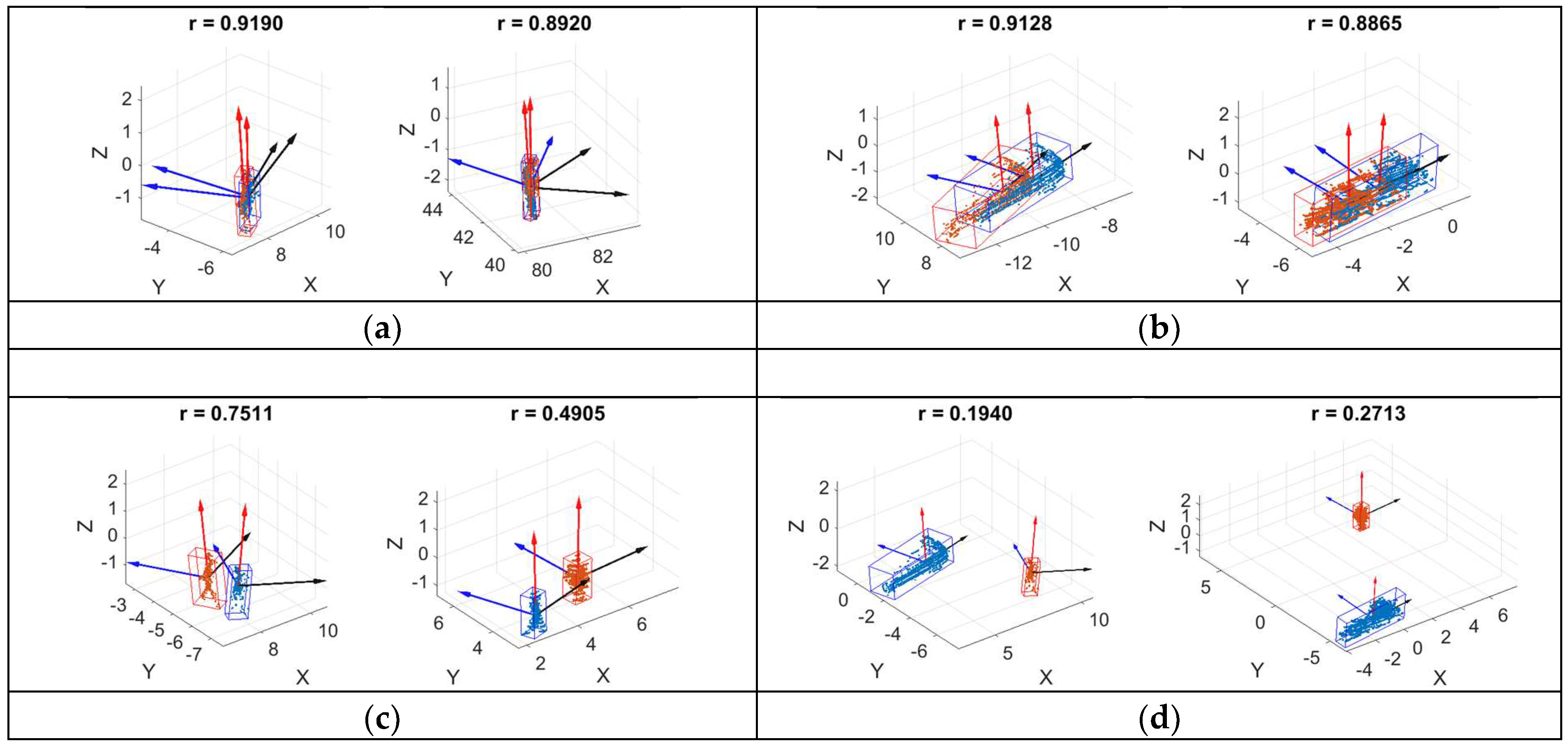
4.4. Feature Description of Point Clouds of Objects
4.5. Managing and Confirming Track Hypotheses
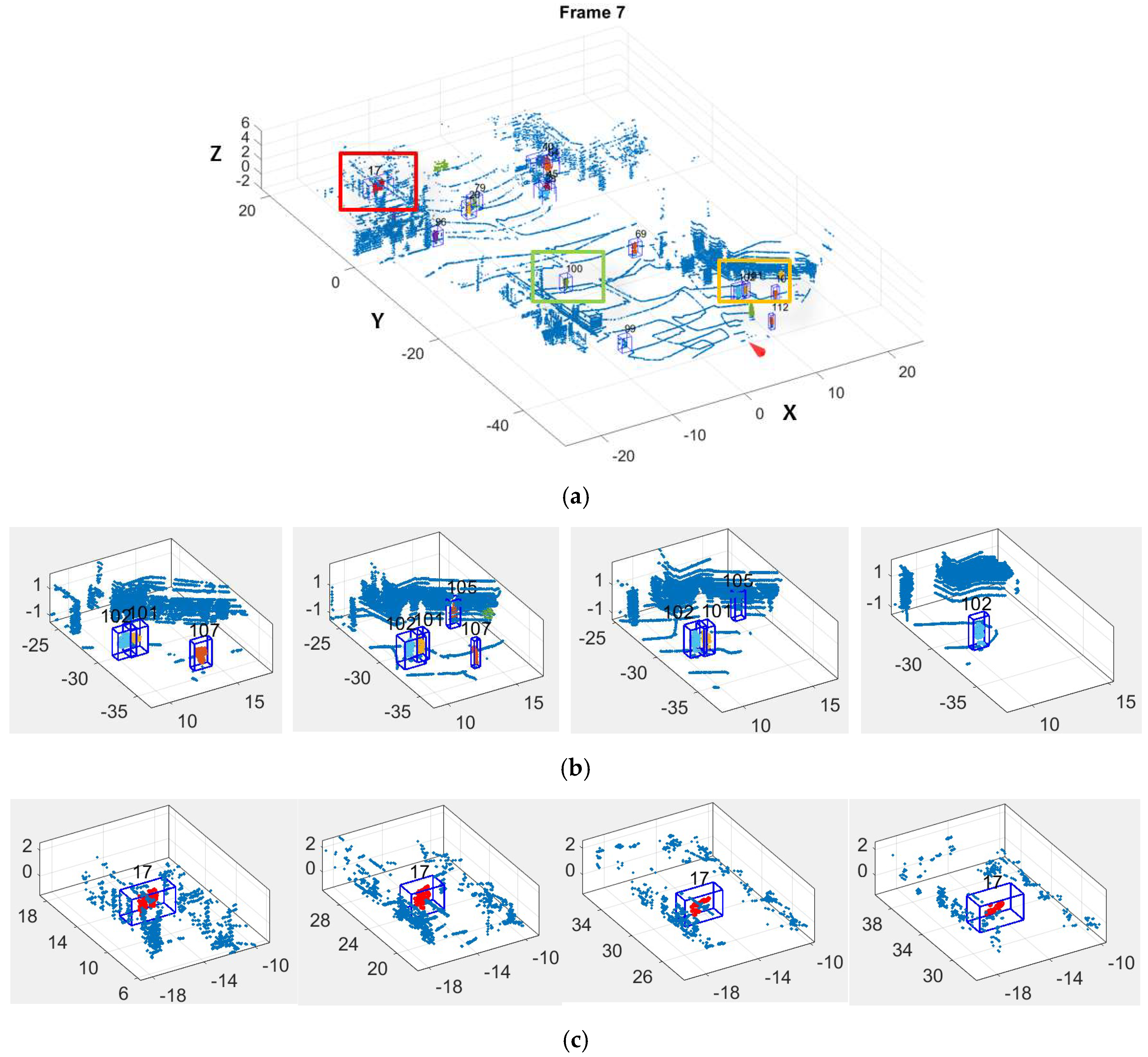
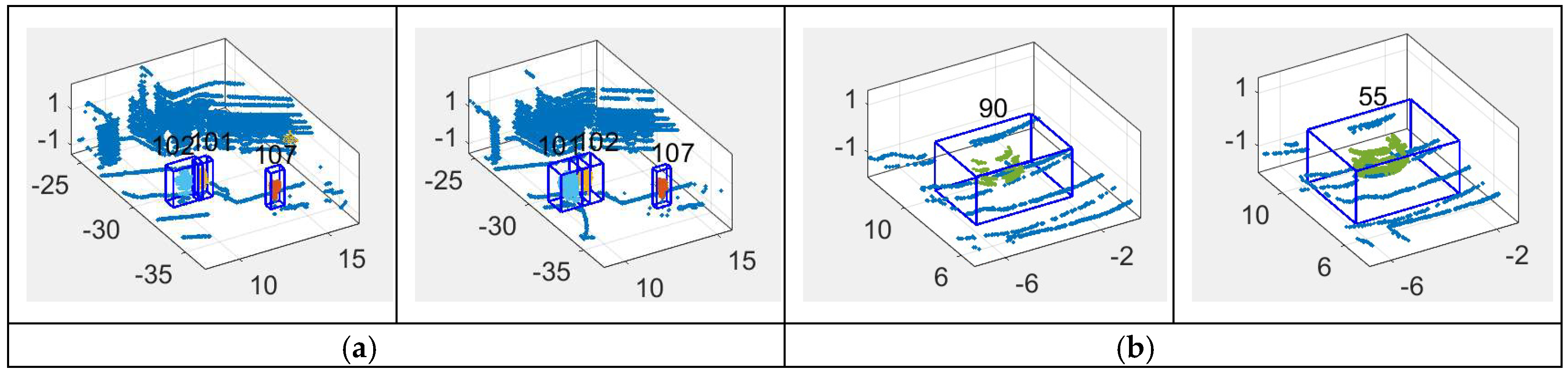
5. Experiments and Evaluations
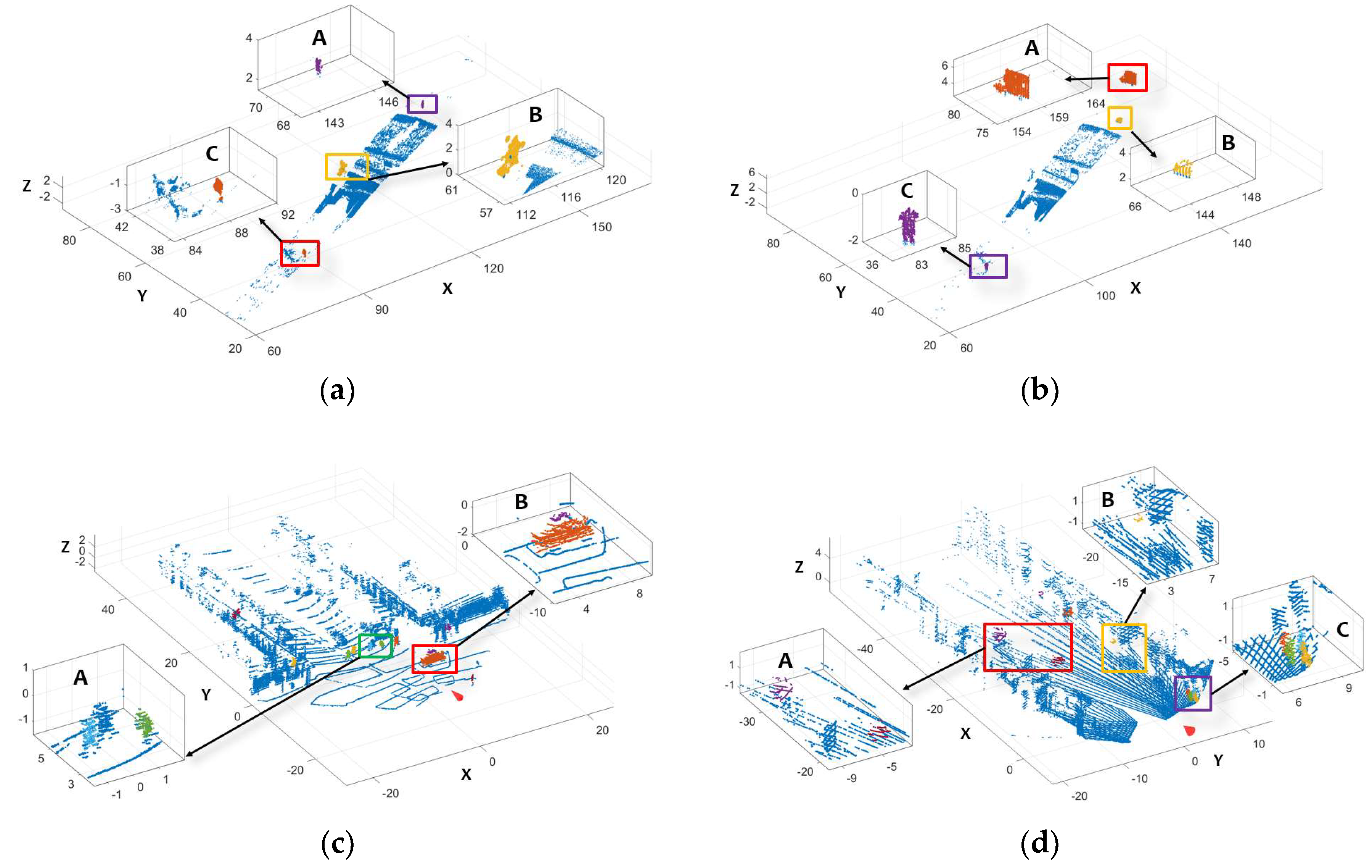
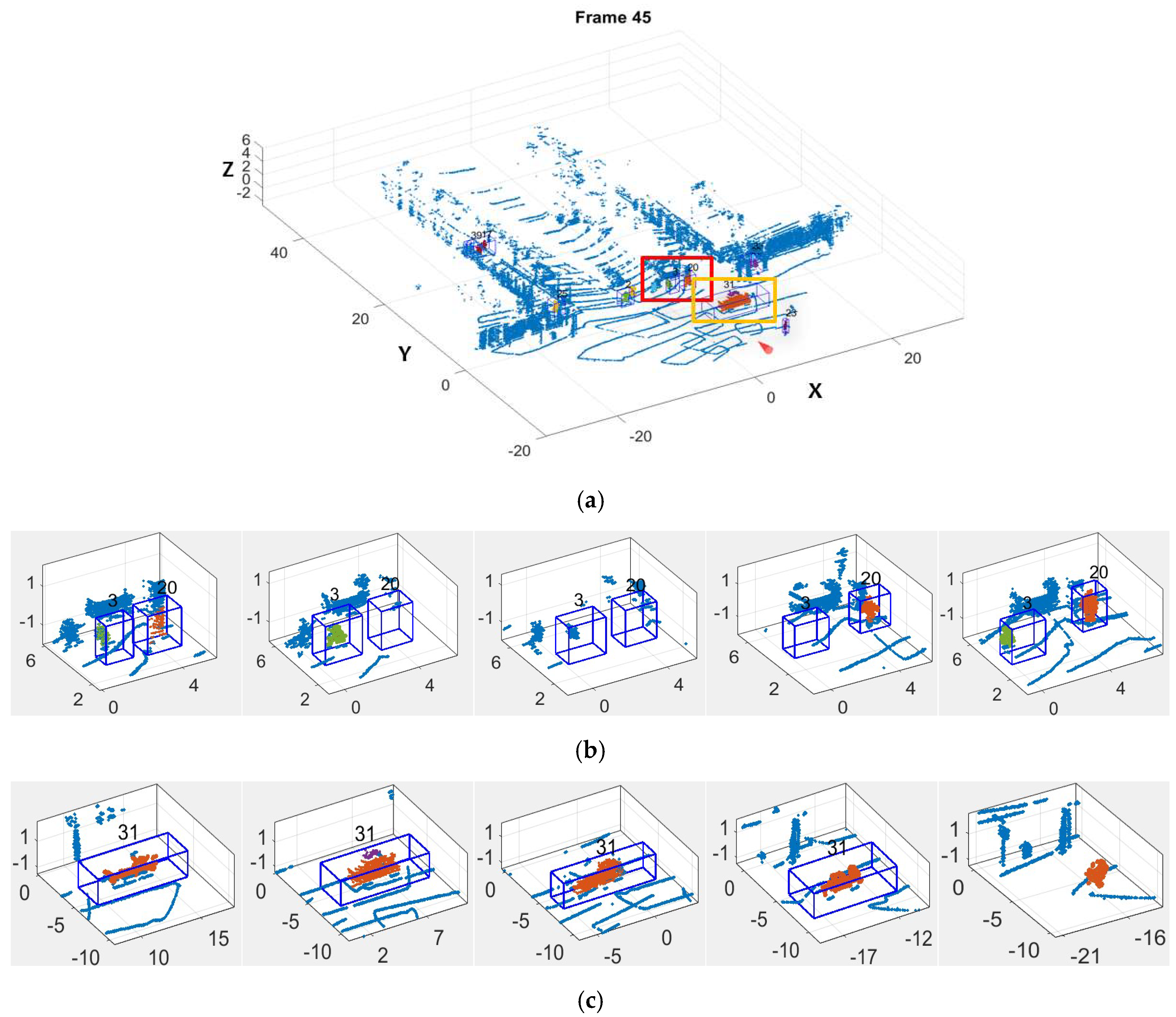
5.1. Moving Object Detection
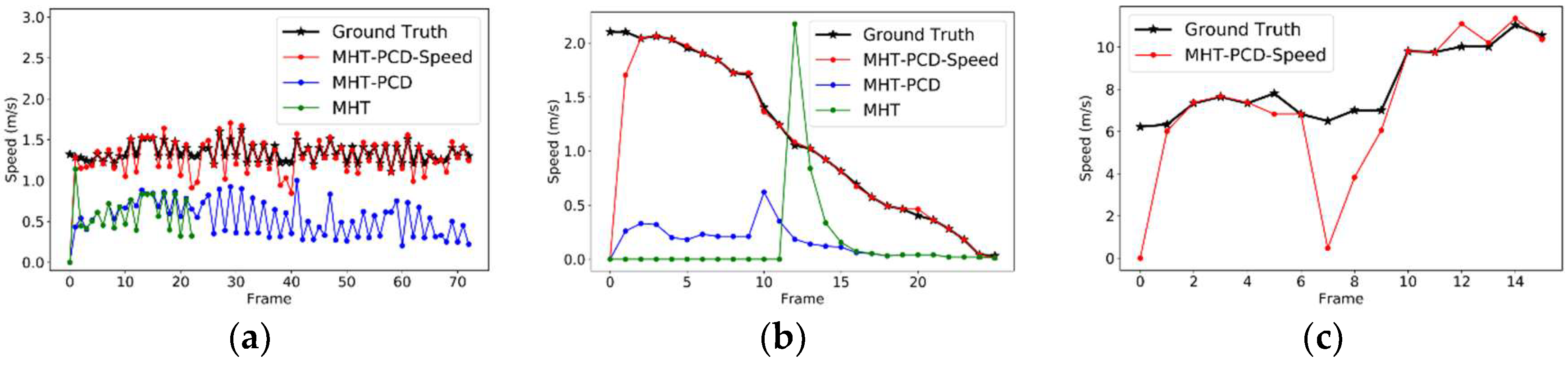
5.2. Moving Object Tracking
6. Conclusions
- The study reveals that the use of Doppler images can enhance the tracking reliability and increase the precision of dynamic state estimation;
- In detection, moving objects are clustered and segmented based on speed information with an adaptive ST-DBSCAN and a region growing technique. The detection method doesn’t require multiple sequential frames of point clouds as input;
- In tracking, the dynamic state of moving objects is estimated with position observation and speed observation, increasing the precision of dynamic state estimation on moving objects, especially those whose speed is changing fast;
- A point cloud descriptor, OESF, is proposed and added in the scoring process of MHT, which allows managing tracks not only according to spatial closeness but also similarity in structure of detections in neighboring frames.
Author Contributions
Funding
Conflicts of Interest
References
- Pourezzat, A.A.; Sadabadi, A.A.; Khalouei, A.; Attar, G.T.; Kalhorian, R. Object Tracking: A Survey. Adv. Environ. Biol. 2013, 7, 253–259. [Google Scholar]
- Prajapati, D.; Galiyawala, H.J. A Review on Moving Object Detection and Tracking. Int. J. Comput. Appl. 2015, 5, 168–175. [Google Scholar]
- Schindler, K.; Ess, A.; Leibe, B.; Van Gool, L. Automatic detection and tracking of pedestrians from a moving stereo rig. ISPRS J. Photogramm. Remote Sens. 2010, 65, 523–537. [Google Scholar] [CrossRef]
- Cao, Y.; Guan, D.; Wu, Y.; Yang, J.; Cao, Y.; Yang, M.Y. Box-level segmentation supervised deep neural networks for accurate and real-time multispectral pedestrian detection. ISPRS J. Photogramm. Remote Sens. 2019, 150, 70–79. [Google Scholar] [CrossRef]
- Luo, H.; Li, J.; Chen, Z.; Wang, C.; Chen, Y.; Cao, L.; Teng, X.; Guan, H.; Wen, C. Vehicle Detection in High-Resolution Aerial Images via Sparse Representation and Superpixels. IEEE Trans. Geosci. Remote Sens. 2015, 54, 103–116. [Google Scholar]
- Kim, C.; Li, F.; Ciptadi, A.; Rehg, J.M. Multiple Hypothesis Tracking Revisisted. In Proceedings of the 2015 IEEE International Conference on Computer Vision (ICCV), Santiago, Chile, 7–13 December 2015. [Google Scholar]
- Spinello, L.; Triebel, R.; Siegwart, R. Multimodal People Detection and Tracking in Crowded Scenes. In Proceedings of the Twenty-Third AAAI Conference on Artificial Intelligence, Chicago, IL, USA, 13–17 July 2008; pp. 1409–1414. [Google Scholar]
- Kaestner, R.; Maye, J.; Pilat, Y.; Siegwart, R. Generative object detection and tracking in 3d range data. In Proceedings of the 2012 IEEE International Conference on Robotics and Automation, Saint Paul, MN, USA, 14–18 May 2012; IEEE: Piscataway, NJ, USA; pp. 3075–3081. [Google Scholar]
- Dewan, A.; Caselitz, T.; Tipaldi, G.D.; Burgard, W. Motion-based detection and tracking in 3D LiDAR scans. In Proceedings of the 2016 IEEE International Conference on Robotics and Automation (ICRA), Stockholm, Sweden, 16–21 May 2016; pp. 4508–4513. [Google Scholar]
- Cui, J.; Zha, H.; Zhao, H.; Shibasaki, R. Laser-based detection and tracking of multiple people in crowds. Comput. Vis. Image Underst. 2007, 106, 300–312. [Google Scholar] [CrossRef]
- Brock, O.; Trinkle, J.; Ramos, F. Model Based Vehicle Tracking for Autonomous Driving in Urban Environments. MIT Press 2009, 1, 175–182. [Google Scholar]
- Wang, H.; Wang, B.; Liu, B.; Meng, X.; Yang, G. Pedestrian recognition and tracking using 3D LiDAR for autonomous vehicle. Rob. Auton. Syst. 2017, 88, 71–78. [Google Scholar] [CrossRef]
- Xiao, W.; Vallet, B.; Schindler, K.; Paparoditis, N. Simultaneous detection and tracking of pedestrian from panoramic laser scanning data. ISPRS Ann. Photogramm. Remote Sens. Spat. Inf. Sci. 2016, 3, 295–302. [Google Scholar] [CrossRef]
- Yan, Z.; Duckett, T.; Bellotto, N. Online learning for human classification in 3D LiDAR-based tracking. In Proceedings of the 2017 IEEE/RSJ International Conference on Intelligent Robots and Systems (IROS), Vancouver, BC, Canada, 24–28 September 2017. [Google Scholar]
- Yang, S.; Wang, C. Simultaneous egomotion estimation, segmentation, and moving object detection. J. F. Robot. 2011, 28, 565–588. [Google Scholar] [CrossRef]
- Schauer, J.; Nüchter, A. Removing non-static objects from 3D laser scan data. ISPRS J. Photogramm. Remote Sens. 2018, 143, 15–38. [Google Scholar] [CrossRef]
- Salti, S.; Tombari, F.; Di Stefano, L. SHOT: Unique signatures of histograms for surface and texture description. Comput. Vis. Image Underst. 2014, 125, 251–264. [Google Scholar] [CrossRef]
- Moosmann, F.; Stiller, C. Joint self-localization and tracking of generic objects in 3D range data. In Proceedings of the 2013 IEEE International Conference on Robotics and Automation, Karlsruhe, Germany, 6–10 May 2013; pp. 1146–1152. [Google Scholar]
- Yu, Y.; Li, J.; Guan, H.; Wang, C. Automated Detection of Three-Dimensional Cars in Mobile Laser Scanning Point Clouds Using DBM-Hough-Forests. IEEE Trans. Geosci. Remote Sens. 2016, 54, 4130–4142. [Google Scholar] [CrossRef]
- Yokoyama, H.; Date, H.; Kanai, S.; Takeda, H. Detection and classification of pole-like objects from mobile laser scanning data of urban environments. Int. J. Cad/Cam 2013, 13, 31–40. [Google Scholar]
- Anderson, J.; Massaro, R.; Curry, J.; Reibel, R.; Nelson, J.; Edwards, J. LADAR: Frequency-Modulated, Continuous Wave LAser Detection And Ranging. Photogramm. Eng. Remote Sens. 2017, 83, 721–727. [Google Scholar] [CrossRef]
- Halmos, M.J.; Henderson, D.M. Pulse compression of an FM chirped CO 2 laser. Appl. Opt. 1989, 28, 3595–3602. [Google Scholar] [CrossRef]
- Slotwinski, A.R.; Goodwin, F.E.; Simonson, D.L. Utilizing GaalAs Laser Diodes As A Source For Frequency Modulated Continuous Wave (FMCW) Coherent Laser Radars. In Laser Diode Technology and Applications; International Society for Optics and Photonics: Bellingham, WA, USA, 1989; pp. 245–252. [Google Scholar]
- Reid, D.B. An Algorithm for Tracking Multiple Targets. IEEE Trans. Automat. Contr. 1979, 24, 843–854. [Google Scholar] [CrossRef]
- Amditis, A.; Thomaidis, G.; Maroudis, P.; Lytrivis, P.; Karaseitanidis, G. Multiple Hypothesis Tracking Implementation. Laser Scanner Technol. 2012. [Google Scholar]
- Ester, M.; Kriegel, H.-P.; Sander, J.; Xu, X. A density-based algorithm for discovering clusters in large spatial databases with noise. In Proceedings of the Kdd, Portland, OR, USA, 2–4 August 1996; Volume 96, pp. 226–231. [Google Scholar]
- Birant, D.; Kut, A. ST-DBSCAN: An algorithm for clustering spatial–temporal data. Data Knowl. Eng. 2007, 60, 208–221. [Google Scholar] [CrossRef]
- Pingel, T.J.; Clarke, K.C.; McBride, W.A. An improved simple morphological filter for the terrain classification of airborne LIDAR data. ISPRS J. Photogramm. Remote Sens. 2013, 77, 21–30. [Google Scholar] [CrossRef]
- Blackman, S.; Popoli, R. Design and Analysis of Modern Tracking Systems (Artech House Radar Library); Artech House: Norwood, MA, USA, 1999. [Google Scholar]
- Fortmann, T.; Bar-Shalom, Y.; Scheffe, M. Sonar tracking of multiple targets using joint probabilistic data association. IEEE J. Ocean. Eng. 1983, 8, 173–184. [Google Scholar] [CrossRef]
- Yilmaz, A.; Javed, O.; Shah, M. Object tracking: A survey. Acm Comput. Surv. 2006, 38, 13. [Google Scholar] [CrossRef]
- Wohlkinger, W.; Vincze, M. Ensemble of shape functions for 3D object classification. In Proceedings of the 2011 IEEE International Conference on Robotics and Biomimetics, Phuket, Thailand, 7–11 December 2011; pp. 2987–2992. [Google Scholar]
- Osada, R.; Funkhouser, T.; Chazelle, B.; Dobkin, D. Matching 3D models with shape distributions. In Proceedings of the International Conference on Shape Modeling and Applications, Genova, Italy, 7–11 May 2001; pp. 154–166. [Google Scholar]
- Geiger, A.; Lenz, P.; Urtasun, R. Are we ready for autonomous driving? the kitti vision benchmark suite. In Proceedings of the 2012 IEEE Conference on Computer Vision and Pattern Recognition (CVPR), Providence, RI, USA, 16–21 June 2012; pp. 3354–3361. [Google Scholar]
- Papageorgiou, D.J.; Salpukas, M.R. The maximum weight independent set problem for data association in multiple hypothesis tracking. In Optimization and Cooperative Control Strategies; Springer: Berlin/Heidelberg, Germany, 2009; pp. 235–255. [Google Scholar]
- Östergård, P.R.J. A new algorithm for the maximum-weight clique problem. Nord. J. Comput. 2001, 8, 424–436. [Google Scholar] [CrossRef]
- Milan, A.; Leal-Taixé, L.; Reid, I.; Roth, S.; Schindler, K. MOT16: A benchmark for multi-object tracking. arXiv 2016, arXiv:1603.00831. [Google Scholar]
- Stiefelhagen, R.; Bernardin, K.; Bowers, R.; Garofolo, J.; Mostefa, D.; Soundararajan, P. The CLEAR 2006 evaluation. In Proceedings of the International Evaluation Workshop on Classification of Events, Activities and Relationships; Springer: Berlin/Heidelberg, Germany, 2006; pp. 1–44. [Google Scholar]


| Dataset | Objects | #Pair of Samples | Mean of | Std. Dev. of |
|---|---|---|---|---|
| KITTI | The Same pedestrian in neighboring frames | 100 | 0.8848/0.9168 | 0.0700/0.0550 |
| Different pedestrians | 100 | 0.8248/0.9543 | 0.1097/0.0262 | |
| The same car in neighboring frames | 50 | 0.9081/0.9241 | 0.0649/0.0741 | |
| Different cars | 150 | 0.7051/0.8412 | 0.1252/0.0772 | |
| Objects in different categories | 200 | 0.1348/0.5219 | 0.0871/0.1706 | |
| Doppler LiDAR | The Same pedestrian in neighboring frames | 100 | 0.8248/0.9543 | 0.1097/0.0262 |
| Different pedestrians | 100 | 0.6466/0.9534 | 0.1442/0.0207 | |
| The same car in neighboring frames | 50 | 0.8016/0.8797 | 0.1297/0.1045 | |
| Different cars | 150 | 0.5617/0.7349 | 0.0967/0.1514 | |
| Objects in different categories | 200 | 0.2191/0.5323 | 0.0593/0.1568 |
| Detection | Tracking | |||||||
|---|---|---|---|---|---|---|---|---|
| Parameter | N | |||||||
| Value | 0.1 | 40 | 0.02s | 3 | 10 | 0.01 | 0.3 | 5 |
| Seq. ID | #Grd TruthObj | #Correct Obj | #Wrong Obj | Precision | Recall | F1 Score | ObjRcl | Sec./Frame | |
|---|---|---|---|---|---|---|---|---|---|
| Terrestrial | A | 107 | 102 | 9 | 0.9189 | 0.9533 | 0.9358 | 0.9667 | 0.65 |
| B | 52 | 48 | 0 | 1 | 0.9231 | 0.9600 | 0.9757 | 0.26 | |
| Mobile | C | 1683 | 1366 | 264 | 0.8380 | 0.8116 | 0.8246 | 0.8089 | 9.39 |
| D | 1230 | 893 | 210 | 0.8096 | 0.7260 | 0.7655 | 0.7347 | 12.97 |
| Method | Seq. | Avg FN | Avg FP | IDSW | MOTA (%) | MT (%) | ML (%) | Sec./Frame |
|---|---|---|---|---|---|---|---|---|
| MHT-PCD-Speed | C | 3.66 | 0.40 | 31 | 76.45 | 66.13 | 9.68 | 1.53 |
| D | 2.25 | 0.75 | 19 | 72.42 | 51.65 | 27.47 | 0.68 | |
| MHT-PCD | C | 3.89 | 0.59 | 35 | 73.96 | 56.45 | 12.90 | 1.59 |
| D | 2.67 | 0.85 | 27 | 67.26 | 43.96 | 28.57 | 0.68 | |
| MHT | C | 4.83 | 0.64 | 37 | 68.55 | 53.23 | 16.13 | 1.54 |
| D | 3.56 | 0.98 | 41 | 57.28 | 41.76 | 32.97 | 0.67 |
| Type | Classification | #Obj | MT (%) | ML (%) |
|---|---|---|---|---|
| Category | Pedestrian | 142 | 56.34 | 20.42 |
| Vehicle | 10 | 51.65 | 20.00 | |
| Bicyclist | 1 | 1 | 0 | |
| Dimension | Small (dx < 0.5 and dy < 0.5) | 140 | 56.42 | 20.00 |
| Large (dx > 0.5 || dy > 0.5) | 13 | 61.54 | 23.08 | |
| Speed | Slow () | 60 | 53.23 | 16.13 |
| Middle () | 70 | 41.76 | 32.97 | |
| Fast () | 18 | 33.33 | 5.56 | |
| Changing rapidly | 5 | 40.00 | 20.00 |
© 2019 by the authors. Licensee MDPI, Basel, Switzerland. This article is an open access article distributed under the terms and conditions of the Creative Commons Attribution (CC BY) license (http://creativecommons.org/licenses/by/4.0/).
Share and Cite
Ma, Y.; Anderson, J.; Crouch, S.; Shan, J. Moving Object Detection and Tracking with Doppler LiDAR. Remote Sens. 2019, 11, 1154. https://doi.org/10.3390/rs11101154
Ma Y, Anderson J, Crouch S, Shan J. Moving Object Detection and Tracking with Doppler LiDAR. Remote Sensing. 2019; 11(10):1154. https://doi.org/10.3390/rs11101154
Chicago/Turabian StyleMa, Yuchi, John Anderson, Stephen Crouch, and Jie Shan. 2019. "Moving Object Detection and Tracking with Doppler LiDAR" Remote Sensing 11, no. 10: 1154. https://doi.org/10.3390/rs11101154
APA StyleMa, Y., Anderson, J., Crouch, S., & Shan, J. (2019). Moving Object Detection and Tracking with Doppler LiDAR. Remote Sensing, 11(10), 1154. https://doi.org/10.3390/rs11101154