Article

Evaluation of Sub-Kilometric Numerical Simulations of C-Band Radar Backscatter over the French Alps against Sentinel-1 Observations

1
Univ. Grenoble Alpes, Université de Toulouse, Météo-France, CNRS, CNRM, Centre d'Etudes de la Neige, 38000 Grenoble, France
2
Centre for Hydrology, University of Saskatchewan, Saskatoon, SK S7N 5C8, Canada
*
Author to whom correspondence should be addressed.
Remote Sens. 2019, 11(1), 8; https://doi.org/10.3390/rs11010008
Submission received: 29 October 2018 / Revised: 17 December 2018 / Accepted: 18 December 2018 / Published: 20 December 2018
(This article belongs to the Special Issue Microwave Remote Sensing for Hydrology)

Abstract

:
This study compares numerical simulations and observations of C-band radar backscatter in a wide region (2300 km 2 ) in the Northern French Alps. Numerical simulations were performed using a model chain composed of the SAFRAN meteorological reanalysis, the Crocus snowpack model and the radiative transfer model Microwave Emission Model for Layered Snowpacks (MEMLS3&a), operating at a spatial resolution of 250-m. The simulations, without any bias correction, were evaluated against 141 Sentinel-1 synthetic aperture radar observation scenes with a resolution of 20 m over three snow seasons from October 2014 to June 2017. Results show that there is good agreement between observations and simulations under snow-free or dry snow conditions, consistent with the fact that dry snow is almost transparent at C-band. Under wet snow conditions, although the changes in time and space are well correlated, there is a significant deviation, up to 5 dB, between observations and simulations. The reasons for these discrepancies were explored, including a sensitivity analysis on the impact of the liquid water percolation scheme in Crocus. This study demonstrates the feasibility of performing end-to-end simulations of radar backscatter over extended geographical region. This makes it possible to envision data assimilation of radar data into snowpack models in the future, pending that deviations are mitigated, either through bias corrections or improved physical modeling of both snow properties and corresponding radar backscatter.

Graphical Abstract

1. Introduction

Monitoring and predicting snow conditions in mountain regions is critical for avalanche forecasting, water resource and flood risk management, and mountain tourism activities. Given the high variability of snow properties over time and space, high resolution information is essential in both dimensions. Remote sensing has been used for decades as a complement for the limited number of in-situ observations. This takes advantage of the peculiar optical and microwave signatures of snow, compared to other Earth surface bodies, providing rich information content to remotely sensed snow observations [1,2,3]. Because they operate in the microwave spectral domain and are not sensitive to clouds, space-borne synthetic aperture radars (SARs) have long been considered for snow monitoring, although this is scientifically and technically challenging. Intrinsically, SAR are a coherent imaging system (all the rays are in phase) with a noise limit defined by the speckle effects (granulation in the image that results from interference between the signals received from the many individual scatterers that contribute to a single target pixel and interfere with the readability of the image and degrade its radiometric resolution). SAR systems have an oblique viewing geometry causing some geometric and radiometric distortions to images, especially for mountainous areas, which must be specifically handled.
Microwave backscatter coefficients over snow result from the combination of several phenomena including reflection on the snow surface, scattering within the snowpack and reflection at the snow–soil boundary. This depends, in particular, on internal snow properties such as the layering of microstructure variables (density, specific surface area, etc.) and liquid water content [4]. In the case of dry snow, C-band radiation penetrates into the snowpack because the dielectric contrast at the air–snow interface is very small and backscattering at the air–snow interface is negligible. Volume scattering is also quite small but increases with snow depth because of signal attenuation and the contribution of the soil to total backscatter decreases. Backscatter coefficients are very sensitive to the presence of liquid water in the snowpack due to the high dielectric contrast between ice and water in the microwave spectrum [5]. Therefore, X- and C-band SAR data have long been used primarily for wet-snow mapping, i.e. identifying pixels where the snowpack contains some liquid water at the time of observation. The relationship between backscatter and snow wetness is mainly controlled by the scattering mechanism. When the surface is smooth, volume scattering is the dominant source of signal, a negative correlation is then observed between the backscatter values and the snow wetness [6,7]. When the surface is rough, surface scattering becomes the dominant diffusion process. Previous studies have demonstrated the capability of C-band European Remote Sensing Satellites (ERS-1 and 2) SARs [8,9], C-band Spaceborne Imaging Radar (SIR-C) and X-band X-SAR [10] and C-band RADARSAT SAR data [11,12] to discriminate wet snow from dry snow or from ground surfaces [13].
The exploitation of C-band SAR signals over snow can proceed further than mapping of wet snow. Inferring other snow properties, such as snow depth, mass or internal properties, can either be performed through geophysical retrievals [14,15,16,17,18] or data assimilation using snowpack models [4,19]. In both cases, this requires a quantitative understanding of the relationships between snow properties and SAR signal. Along with other satellite observations [20,21], there is hope that data assimilation in detailed snowpack models can improve our snow monitoring and prediction capabilities, especially at high elevation where in-situ observations are particularly scarce [3]. Several surface and volume scattering models have been developed since the 1980s [22] addressing either the passive or active microwave behavior of snow. Recently, the Microwave Emission Model for Layered Snowpacks (MEMLS) [23], initially devoted to passive microwave signals, was extended to computing radar backscatter (MEMLS3&a) [24]. The passive microwave implementation of MEMLS has previously been driven by snowpack model output [25,26]) or in-situ snow measurements [27]. Recent studies have driven MEMLS3&a with in-situ snow measurements to feed the model and to compare with SAR measurements [28,29]. However, most previous studies were carried out at the point scale, using in-situ snow observations or using in-situ meteorological observations to drive snowpack models, and comparing to in-situ SAR observations rather than from satellite-borne sensors. While they demonstrated potential in using such data for larger scale use operationally, few studies have attempted to simulate explicitly radar backscatter at the regional scale, although this is a prerequisite for data assimilation in snowpack models.
This study introduced a model chain that uses the SAFRAN-Crocus state-of-the-art multi-layer snowpack model [30,31,32] as input to the radiative transfer model MEMLS3&a [24] to simulate backscatter coefficients at C-band over a large alpine region. Simulations were compared to observations from the European Space Agency’s (ESA) Copernicus (European Union’s Earth Observation Programme) Sentinel-1 sensor (VV and VH polarizations). The study spanned three seasons (2014–2015, 2015–2016 and 2016–2017) involving the processing and use of 141 Sentinel-1 images over an area of 2310 km 2 at a spatial resolution of 250 m. To our knowledge, this is the first study of this extent on the Alps.
Data and models used in this study are described in Section 2. Results are provided in Section 3, while Section 4 provides discussion and conclusions.

2. Data and Models

Our study area is located in the French Alps. This alpine area, shown in Figure 1, has an area of 2310 km 2 with several land cover types (see Figure 2), complex topography (valleys to high mountain) and snow conditions. Moreover, the site is at the intersection of several massifs (Grandes-Rousses, Tabor, Oisans, Pelvoux, Devoluy, Champsaur, Belledonne and Maurienne) and includes the Col du Lautaret, which is a snow measurement site. The period of study was from October 2014 to July 2017. To characterize surface types, we used high resolution (25 m) land cover products from the CORINE Land Cover (CLC) European database (see http://www.statistiques.developpement-durable.gouv.fr/clc). Figure 2 shows the site surface types including forests, bare ground, glaciers and wetlands. Land use and relief of the study zone make it a very representative area of the Alps. The analysis is restricted to the following surface types: natural grassland, moors and heathland, bush vegetation, bare rock, sparsely vegetated areas, glacier and perpetual snow. Other surface types, such as forests and urban areas, are excluded from the analysis because the snowpack model used does not account for these situations.

2.1. Sentinel-1 Data

We used backscatter coefficients at C-band from the SAR on board Sentinel-1 missions operated by the ESA within the Copernicus programme. The Sentinel-1 mission consists of a constellation of two satellites, Sentinel-1A and Sentinel-1B, which are 180° orbit apart, allowing observations of the French Alps every six days. Sentinel-1A and Sentinel-1B were launched in April 2014 and April 2016, respectively.
Sentinel-1 has a side-looking imaging geometry and images are subject to geometric distortions including shadow, layover and foreshortening effects [33]. Since SAR observations are strongly influenced by topography, areas with geometric distortions must be identified to be excluded and incidence angles must be corrected using a high resolution digital elevation model (DEM).
We used Level-1 Ground Range Detected (GRD) products made available through the Copernicus web site (https://scihub.copernicus.eu/dhus/). Sentinel-1 data have a spatial resolution of 20 m in both VV and VH polarization. Available Sentinel-1 orbits, ascending and descending, relevant for our study area were selected and pre-processed using the ESA Sentinel-1 Toolbox. The pre-processing includes SAR image extraction over our test zone, thermal noise removal, speckle filtering (using a refined Frost filter [34]), radiometric calibration and terrain correction [35] using the French National Institute for Geographic and Forestry Information (IGN) digital elevation model at 25 m.
The selected Sentinel-1 images from ascending and descending orbits are shown in Table 1. Areas of excessive geometric distortions were identified for each orbit using the Sentinel Application Platform (SNAP) modules and used to screen out pixels associated with geometric distortions. Figure 3 shows SAR backscatter values at VV polarization (in dB) obtained on 13 February 2017 (descending orbit) and on 14 February 2017 (ascending orbit) together with the corresponding geometric distortions mask (displayed in red). For clarity, lakes (in dark blue) and glaciers (in light blue) are also displayed. One could notice that a significant number of pixels was screened out due to geometric distortions, around 14% and 16% of total pixels for ascending and descending images, respectively. Combination of ascending and descending orbits to optimally observe mountains is necessary to overcome the inherent SAR geometric distortions.

2.2. SAFRAN-Crocus

The Crocus snowpack evolution model was used in this study. Crocus is a state-of-the-art unidimensional numerical snowpack model that simulates the time evolution of the snowpack by computing the energy and mass balance of the snowpack [30,31]. Crocus performs simulations with a detailed description of the vertical stratification of the snowpack by using a Lagrangian vertical discretization, and simulates the evolution of the physical properties of each snow layer taking into account its metamorphism [32].
Crocus is one of the snowpack models within the land surface model ISBA-DIF (Interaction between Soil, Biosphere and Atmosphere; diffusion version) [36,37], which allows for the thermodynamical coupling between snow and soil models. Crocus can be forced by observations, forecasts, analyses or reanalyses or coupled to atmospheric models. In this study, Crocus was fed by re-analysis fields from the atmospheric analysis system SAFRAN [38,39]. SAFRAN provides hourly surface meteorological information over massifs (23 massifs in the French Alps and 23 massifs in the Pyrenees), for which the spatial variability of meteorological conditions is assumed to only depend on elevation, using 300-m elevation steps. The meteorological variables are surface air temperature and humidity, wind speed, precipitation rate, precipitation phase, and downward longwave and shortwave radiative fluxes (direct and scattered).

2.3. MEMLS3&a

The C-band backscatter of the snowpack was simulated using MEMLS3&a [24]. MEMLS is based on a six-flux theory which takes into account the description of the multiple volume scattering, the absorption, internal reflection trapping and a combination of coherent and incoherent superposition of reflections between the different layers of the snowpack [23,24]. The snowpack is considered as a stack of layers with planar boundaries for both the ground–snow and snow–air interfaces. Each layer is described by physical properties of the snow (temperature (T), volumetric liquid water content (LWC v o l ), density ( ρ ), layer thickness (d), and exponential correlation length (l e x t )) provided directly or indirectly by Crocus simulation output. The exponential correlation length is calculated using ice density and the snow specific surface area (SSA) [24] from Crocus output. MEMLS3&a was also fed with the soil temperature and moisture of the first layer of the soil in ISBA-DIF output. The snow-ground reflectivity was estimated using a dedicated model [40]. It uses the frequency of acquisition, local incidence angle, soil surface height and dielectric constant. The latter one is calculated using a dielectric model for moist soils with clay content and soil moisture of the first soil layer from ISBA-DIF, as inputs [41]. For snow-free simulations, we used MEMLS3&a with only one dry snow layer with T s n o w = 263 K, LWC v o l = 0% vol, ρ = 130 kg m 3 and d = 1 cm so that the snow has a negligible impact on the C-band backscatter values. Instrumental parameters such as frequency, polarization, and incidence angle for each pixel, depending on the observation configuration and pixel orientation, were also used as inputs to run MEMLS3&a.

2.4. Model Configuration and Simulation Setups

Meteorological reanalysis fields from SAFRAN were generated for the period ranging from 1 October 2014 to 1 August 2017 with an output time step of 1 h and were then spatially distributed over a 250 m × 250 m grid spacing with the IGN digital elevation model and for the study area. The entire process provides a set of 250-m gridded atmospheric forcings, which were then used to feed the snow model Crocus and to obtain gridded snowpack simulations [42,43]. The main added value of the high resolution is the correction of incoming solar radiations due to the shadows of the surrounding topography [43,44].
In addition to the simulations performed in the full domain, we also focused on two additional model geographic configurations. First, we focused on a flat area at 2900 m elevation, which can be observed through both ascending and descending observing configuration. This area corresponds to 20 radar pixels (20 m × 20 m size) and one single 250 m resolution model grid point. Model output were also specifically considered at two locations where in-situ observations are performed: Les Ecrins (2978 m) and Meije-Nivose (3100 m). In this case, we use observations from neighbouring radar pixel and one dedicated simulation point matching the topographical configuration of these locations. Note that the Meije-Nivose location can only be observed through ascending orbits, and Ecrins location can only be observed through descending orbits. The 2900 m area and the two point-scale locations are displayed on Figure 2.
We used the default physical options for all processes [45] except for liquid water percolation. For liquid water percolation in the snowpack, we performed simulations using the default version of Crocus (called hereafter B92) for which the volumetric liquid water-holding capacity is defined by a fixed maximal percentage of the pores volumes [46]. We performed simulations with two other liquid water percolation parameterizations: SPK, the bucket version of the SNOWPACK model [45,47] and B02 the ISBA-ES formulation [45,48]. We initialized the soil temperature by generating a spin-up of the temperature profile over our three-year period (2014–2017). Finally, Crocus was run with a maximum number of 20 layers to reduce the numerical cost of microwave emission modeling compared to the 50 layers default configuration.

2.5. Evaluation

In this study, we evaluated backscatter simulations at C-band over an alpine snow covered terrain using a succession of dates (141 SAR images between 2014 and 2017) for which the area is partially or almost completely covered by snow. Numerical simulations of C-band backscatter values were computed for all days of simulation at 6:00 and 18:00 UTC to match the Sentinel-1 observation times (see Figure 4). To be able to properly compare the 250-m simulations with the 20-m observations date by date and to keep the accuracy of the geometric distortions mask, the simulations were geo-located compared to the observations and then resampled to the same geometry. The final product is a stack of both observations and simulations which can be easily compared.
Simulation results in terms of backscatter values were compared to observations, for the full domain, the sub-domain or the two point locations. Statistics quantifying the level of agreement of these two independent sources of information were computed (Pearson correlation coefficients and normalized standard deviation). Note that, because of their topographical configuration, Les Ecrins and Meije-Nivose were only handled for descending and ascending orbits, respectively. Additional SAFRAN-Crocus simulation output (snow water equivalent (SWE) and maximum value of the liquid water content (LWC) of snow layers at a given location) were used to provide context to the analysis of backscatter data. This makes it possible to identify pixels which are, according to SAFRAN-Crocus output, without snow (snow-free), dry if the LWC is equal to 0 and wet if at least one of the snowpack layers has a liquid water content above 0% vol.

3. Results

3.1. Snow-Free Situations

Figure 5 provides results from four different snow free dates (13 July 2016 and 18 August 2016 for ascending orbit and 18 July 2015 and 16 September 2015 for descending orbit). The figure shows the distributions of simulated (in dark grey) and observed backscatter values (light grey) for the four selected dates. The distributions of simulated backscatter values show smaller variability than those of the observations. For both orbit types, the simulated backscatter values are ranging from −50 dB to 5 dB for VV polarization and from −50 dB to −10 dB for VH polarization. The observed backscatter values are ranging from −30 dB to 5 dB for VV polarization and from −30 dB to 0 dB for VH polarization. For the ascending orbit, the central values of the simulated and observed distributions are separated by 6 dB for VV and VH polarization. For the descending orbit, Figure 5b shows a deviation of 5 dB between the central values for observations and simulations for both polarizations.

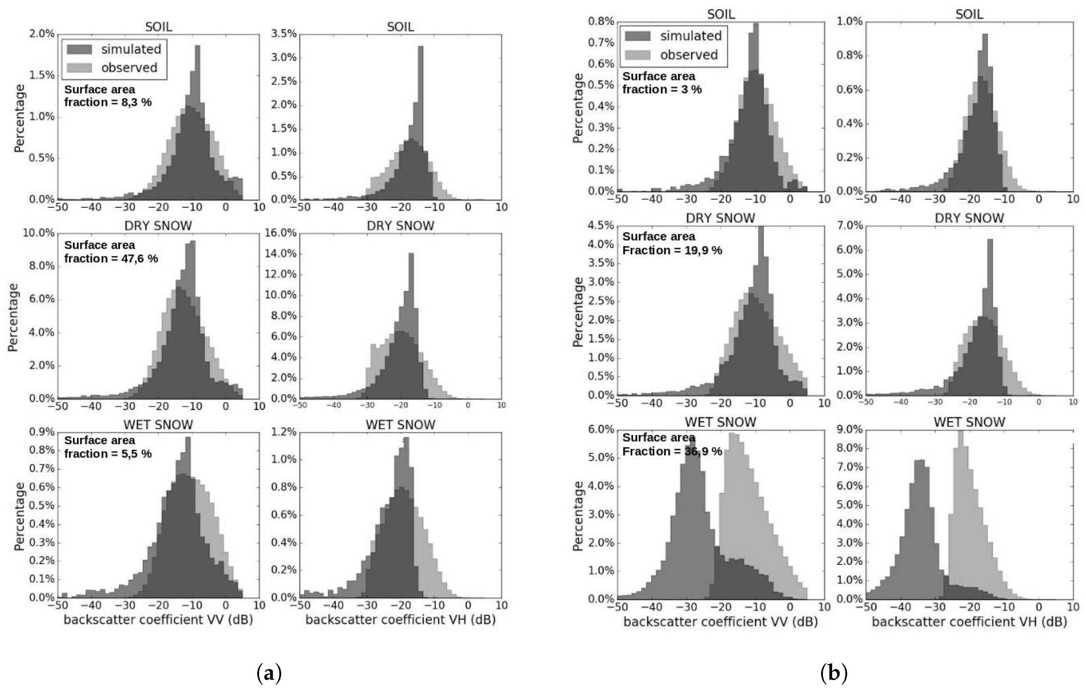
3.2. Comparisons over the Full Domain

Figure 6 compares simulations (in dark grey: VV left side and VH right side) with observed backscatter values (in light grey: VV left side and VH right side) for snow free situations (top), dry snow (middle) and wet snow (bottom) for two contrasted dates. The two selected dates are representative of the beginning of the snow season (10 December 2015) and of a melting period (1 April 2015). Backscatter values range from −25 dB to 3 dB for VV polarization and −30 dB to −2 dB for VH polarization for the observations, whereas simulations range from −40 dB to 2 dB for VV polarization and −45 dB to −10 dB for VH polarization. For snow-free situations, the central values of the observed and simulated distributions for both orbit types are separated by less than 2 dB and, for dry snow, they are separated by 5 dB. One can notice that the distributions for snow free and dry snow cases are similar to the ones observed in summer in Figure 5. This behavior was expected since dry snow is almost transparent at C-band. In the case of wet snow, the backscatter values of the simulations range from −50 to 5 dB for both dates in VV polarization and from −50 dB to −10 dB in VH polarization. The figure shows a deviation between the simulations and observations distributions especially for 1 April 2015 with a 15 dB deviation. In this specific case, we note that the two selected situations not only correspond to two different orbit configurations (ascending vs. descending, so that different locations are actually considered given the rugged topography) but also two different dates (at different observation times, morning vs. afternoon), with very different snow conditions. This illustrates the difficulty to understand the reason for the discrepancy between observations and simulations in these cases.
Pearson correlation coefficients for both orbits, VV and VH polarizations and seven different elevation ranges are summarized in Table 2. There are higher correlation coefficients for elevations between 2250 m and 3150 m (ranging from 0.52 to 0.86) for ascending orbit and both polarizations and correlation coefficients ranging from 0.31 to 0.76 for descending orbit and both polarizations.
We investigated the impact of the slope aspect in both orbit types and for the observed and simulated backscatter values for two consecutive dates: 13 February 2017 (descending) and 14 February 2017 (ascending) (see Figure 7). It shows larger differences between observations and simulations for the southwest, west and northwest slope orientations for the descending orbit (Figure 7a) with the central value of the observation and simulation distributions around −17 dB and −10 dB, respectively, while the eastern slope aspect (northeast, east, and southeast) and the south display a better agreement between the distributions. A different behavior was observed in the case of the ascending orbit with larger differences between the distributions for the slope aspects going from north to southeast and a better fit of the simulated and observed distributions for the slope aspects ranging from south to northwest.

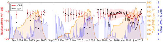
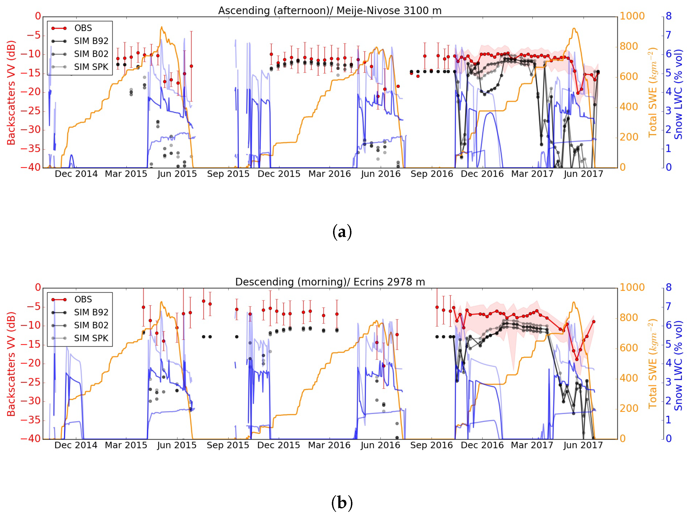
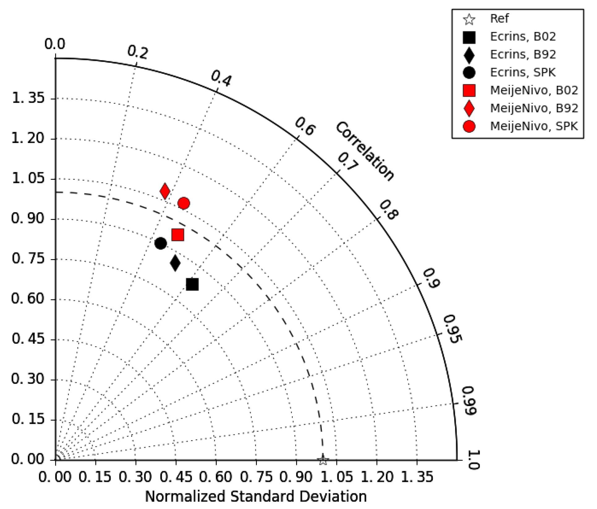
3.3. Comparisons at High Elevation Locations

Figure 8 compares time series of observations and simulations (at VV polarization) on the 2900 m area using ascending (top) and descending orbits (bottom). Information about SWE (dashed area in orange) and LWC (blue line) are also plotted in the same panels. The simulations follow the temporal behavior more than the observations throughout the study period and there are episodes with strong deviation between observations and simulations. During snow free and dry snow periods, the figure shows a deviation of less than 2 dB for most of the dates and for both ascending and descending orbits. The changes of the simulated backscatter values following changes in snowpack conditions follow that of observations but with a larger amplitude of change. Indeed, the figure displays a negative deviation ranging from 5 dB to 25 dB. For the ascending orbit, there is a large decrease of simulated backscatter on 9 March 2015 due to an increase of simulated LWC, which does not show a corresponding decrease in observed backscatter values. For melting season periods (such as from 21 March 2015 to 13 June 2015), we observe a decrease in backscatter in both observations and simulations, along with increasing SWE. Some isolated episodes of snow melting are well represented with a decrease of backscatter for observations and simulations (see for instance October 2016 in both orbit types).
Figure 9 illustrates, similarly to Figure 8, the temporal variations of the backscatter values but with a focus on the elevation range between 2850 m and 3150 m (ascending (top) and descending orbits (bottom)). There is a mean deviation of less than 2 dB between observations and simulations with an increase of deviation up to 12 dB during the melting season associated with a strong increase of the snow LWC. The figure shows a larger negative deviation for the descending orbit than for the ascending orbit especially for snow free and dry snow situations. Higher values of maximum snowpack LWC (up to 6.5%) and total SWE (up to 700 kg m 2 ) correspond to minimum values of the backscatter variations and especially in the melting season. As for Figure 8, the simulations follow the temporal behavior of the observations with larger negative biases increasing with the snowpack LWC.

3.4. Influence of Crocus Liquid Water Percolation Parameterizations

We investigated the sensitivity of our results to the parameterization of the liquid water holding capacity.
Figure 10 shows that the maximum snowpack LWC displayed by each percolation parameterization is different. The SPK scheme leads to higher values of snow LWC (that can exceed 6% vol) than the B02 scheme (that do not exceed 2% vol). The default parameterization B92 stands between the other two. When looking at the backscatter simulations, small differences are seen (2–7 dB) between the results obtained using various percolation parameterizations. However, it appears that, for some periods of the snow seasons, the simulations from the B02 parameterization display a better agreement with the observations (for example see the period from November 2016 to January 2017 for the ascending orbit at the Meije-Nivose station in Figure 10a).
Figure 11 illustrates the Taylor diagram for each percolation parameterization and for both in-situ stations.The Ecrins station is represented in black and the Meije-Nivose station in red and the three different schemes of the percolation of liquid water in the snowpack by different markers: square, diamond and circle for B02, B92 and SPK, respectively. For the Ecrins station (descending orbit), the correlations range from 0.41 to 0.61 and the normalized standard deviation (NSTD) from 0.83 to 0.90 and for the Meije-Nivose station (ascending orbit) correlations range from 0.39 to 0.46 and the NSTD from 0.97 to 1.07. For the Ecrins station, the B02 scheme gives the best results (0.61/0.83). These results are not surprising and highlight the link between the liquid water content of the snowpack model and the simulated backscatter values. Note that the three parameterizations rely on the same “bucket” concept and are not sufficient to represent the real uncertainty of liquid water percolation modeling which involves more complex processes (e.g., capillary barriers and three-dimensional runoff [47,49]).

4. Discussion and Conclusions

In this study, we evaluated simulations of the backscatter coefficients obtained using the model chain SAFRAN-Crocus-MEMLS3&a against observation scenes from Sentinel-1 during three snow seasons from October 2014 to June 2017 over a large study area in the French Alps. Simulations were performed at a 250-m resolution, and compared to 141 observation scenes, without any bias correction applied to model results.
For situations with snow free and dry snow, simulations distributions were consistent with the observations. Moreover, we saw a similar behavior of the backscatter values simulated and observed for the two types of surfaces with the C-band, which was observed in previous studies [50], according to the fact that, for C-band and dry snow, the signal is mostly impacted by the underlying ground.
In the case of wet snow, the simulations show large deviations, although the timing of the changes are rather in good agreement compared to the observations. There was generally a negative deviation between simulations and observations during some periods of the snow seasons. The study showed that some of these differences increase with the increasing snowpack liquid water content. This behavior was seen especially during the melting periods of the snow seasons. The liquid water content is known to have a strong impact on the backscatter signal in C-band, as shown previously [8,12,17,51], thus one possible explanation in these cases could be too large quantities of liquid water content computed in Crocus, which could have many origins including errors of the SAFRAN meteorological reanalyses (precipitation, incoming radiation) or errors of the snowpack percolation scheme. Note that the long-term persistence of thick homogeneous wet layers is a model issue commonly raised by avalanche forecasters, which can only be solved in the future by a more physical modeling of liquid water percolation [47,52]). Likewise, the complexity of the topography in the study area is challenging despite the availability of both ascending and descending orbit observation scenes. Indeed, along with the liquid water content, the pixel orientation and slope angle exert significant impact on both simulated and observed backscatter values. Sentinel-1 observations were better simulated notably for elevation ranges above 2200 m. Although the way phase change and liquid water is handled by the snowpack model Crocus is probably one of the reasons for the deviations reported in this study, overall every single step of the entire model chain SAFRAN-Crocus-MEMLS3&a implemented in this study holds some responsibility in the mismatch between observed and simulated backscatter values. The performance of radiative transfer models, such as MEMLS3&a, should be assessed in non-idealized situations, such as those in this study. Future developments could involve the use of alternative observation operators, making it possible to explore other theoretical approaches to microwave radiative transfer [53].
Nevertheless, our study demonstrates that the technology readiness level for forward modeling of C-band backscatter cannot be assessed on the sole basis of studies testing only one of the elements of the full modeling chain. End-to-end prototypes, such as the study reported here, can be deceptive in that they may show that further work is needed to increase the degree of realism of the modeling chain, but this also provides a baseline, which can be used as a foundation for further studies and developments. In its current state, direct data assimilation in this model chain is probably beyond reach. Besides the clear need and potential for improving each individual element and the full model chain (e.g., improved radiative transfer calculations with enhanced surface scattering modeling, and improved physical modeling of snow including time variations of surface roughness and liquid water dynamics in snow), the fact that backscatter observations and simulations show clear correlation in time suggests to also develop bias correction approaches applied to model output, which may enable backscatter data assimilation under the current state of the model chain [54,55]. In all cases, this study represents a major step towards the assimilation of Sentinel-1 SAR data into a snowpack model such as Crocus.

Author Contributions

Research design and supervision, F.K., S.M.; Numerical simulations, G.V. with support from M.L. and V.V. Data processing and result analysis, G.V., F.K.; Writing-Original Draft Preparation: G.V., F.K., S.M.; Writing-Review & Editing: S.M., F.K., G.V.

Funding

This study was co-funded at 50% by the National Centre for Space Studies (CNES) and at 50% by Météo-France.

Acknowledgments

CNRM/CEN is part of Labex OSUG@2020 (Investissements d’avenir—ANR10 LABX56). We thank Ghislain Picard (Univ. Grenoble Alpes, IGE) and Laurent Ferro-Famil (Univ. Rennes, IETR) for useful feedback. We thank three anonymous reviewers for constructive criticisms, which improved the quality of the manuscript.

Conflicts of Interest

The authors declare no conflict of interest.

References

  1. Nolin, A.W. Recent advances in remote sensing of seasonal snow. J. Glaciol. 2010, 56, 1141–1150. [Google Scholar] [CrossRef]
  2. Singh, M.K.; Gupta, R.; Bhardwaj, A.; Joshi, P.K. Remote sensing of mountain snow using active microwave sensors: A review. Geocarto Int. 2015, 30, 1–27. [Google Scholar] [CrossRef]
  3. Bormann, K.; Brown, R.D.; Derksen, C.; Painter, T. Estimating snow-cover trends from space. Nat. Clim. Change 2018, 8. [Google Scholar] [CrossRef]
  4. Phan, X.V.; Ferro-Famil, L.; Gay, M.; Durand, Y.; Dumont, M.; Morin, S.; Allain, S.; D’Urso, G.; Girard, A. 1D-Var multilayer assimilation of X-band SAR data into a detailed snowpack model. Cryosphere 2014, 8, 1975–1987. [Google Scholar] [CrossRef] [Green Version]
  5. Nagler, T.; Rott, H.; Ripper, E.; Bippus, G.; Hetzenecker, M. Advancements for Snowmelt Monitoring by Means of Sentinel-1 SAR. Remote Sens. 2016, 8, 348. [Google Scholar] [CrossRef]
  6. Shi, J.; Dozier, J. Radar backscattering response to wet snow. In Proceedings of the IGARSS’92 Geoscience and Remote Sensing Symposium, Houston, TX, USA, 26–29 May 1992; IEEE: Piscataway, NJ, USA, 1992; Volume 2, pp. 927–929. [Google Scholar]
  7. Rott, H.; Davis, R.E. Multifrequency and polarimetric SAR observations on alpine glaciers. Ann. Glaciol. 1993, 17, 98–104. [Google Scholar] [CrossRef] [Green Version]
  8. Baghdadi, N.; Gauthier, Y.; Bernier, M. Capability of multitemporal ERS-1 SAR data for wet-snow mapping. Remote Sens. Environ. 1997, 60, 174–186. [Google Scholar] [CrossRef]
  9. Koskinen, J.; Metsämäki, S.; Grandell, J.; Jänne, S.; Matikainen, L.; Hallikainen, M. Snow Monitoring Using Radar and Optical Satellite Data. Remote Sens. Environ. 1999, 69, 16–29. [Google Scholar] [CrossRef]
  10. Shi, J.; Dozier, J. Mapping seasonal snow with SIR-C/X-SAR in mountainous areas. Remote Sens. Environ. 1997, 59, 294–307. [Google Scholar] [CrossRef]
  11. Magagi, R.; Bernier, M. Optimal conditions for wet snow detection using RADARSAT SAR data. Remote Sens. Environ. 2003, 84, 221–233. [Google Scholar] [CrossRef]
  12. Baghdadi, N.; Gauthier, Y.; Bernier, M.; Fortin, J.P. Potential and Limitations of RADARSAT SAR Data for Wet Snow Monitoring. IEEE Trans. Geosci. Remote 2000, 38, 316–320. [Google Scholar] [CrossRef]
  13. Rott, H.; Mätzler, C. Possibilities and Limits of Synthetic Aperture Radar for Snow and Glacier Surveying. Ann. Glaciol. 1987, 9, 195–199. [Google Scholar] [CrossRef]
  14. Shi, J.; Dozier, J. Inferring Snow Wetness Using C-Band Data from SIR-C’s Polarimetric Synthetic Aperture Radar. IEEE Trans. Geosci. Remote 1995, 33, 905–914. [Google Scholar]
  15. Besic, N.; Vasile, G.; Chanussot, J.; Stankovic, S.; Dedieu, J.P.; d’Urso, G.; Boldo, D.; Ovarlez, J.P. Dry Snow Backscattering Sensitivity on Density change for SWE Estimation. In Proceedings of the IEEE International Geoscience and Remote Sensing Symposium (IGARSS 2012), Munich, Germany, 22–27 July 2012. [Google Scholar]
  16. Besic, N.; Vasile, G.; Chanussot, J.; Stankovic, S.; Boldo, D.; d’Urso, G. Wet Snow Backscattering Sensitivity on Density change for SWE Estimation. In Proceedings of the IEEE International Geoscience and Remote Sensing Symposium (IGARSS 2013), Melbourne, VIC, Australia, 21–26 July 2013. [Google Scholar]
  17. Longepe, N.; Allain, S.; Ferro-Famil, L.; Pottier, E.; Durand, Y. Snowpack characterization in mountainous regions using C-Band SAR data and a meteorological model. IEEE Trans. Geosci. Remote Sens. 2009, 47, 406–418. [Google Scholar] [CrossRef]
  18. Cui, Y.; Xiong, C.; Lemmetyinen, J.; Shi, J.; Jiang, L.; Peng, B.; Li, H.; Zhao, T.; Ji, D.; Hu, T. Estimating Snow Water Equivalent with Backscattering at X and Ku Band Based on Absorption Loss. Remote Sens. 2016, 8, 505. [Google Scholar] [CrossRef]
  19. Pulliainen, J. Mapping of snow water equivalent and snow depth in boreal and sub-arctic zones by assimilating space-borne microwave radiometer data and ground-based observations. Remote Sens. Environ. 2006, 101, 257–269. [Google Scholar] [CrossRef]
  20. Dumont, M.; Durand, Y.; Arnaud, Y.; Six, D. Variational assimilation of albedo in a snowpack model and reconstruction of the spatial mass-balance distribution of an alpine glacier. J. Glaciol. 2012, 58, 151–164. [Google Scholar] [CrossRef]
  21. Cluzet, B.; Revuelto, J.; Lafaysse, M.; Dumont, M.; Cosme, E.; Tuzet, F. Assimilation of MODIS observations of snowpack surface properties into one year of spatialized ensemble snowpack simulations at a field site in the French Alps. In Proceedings of the ISSW, Innsbruck, Austria, 7–12 October 2018. [Google Scholar]
  22. Ulaby, F.; Moore, R.; Fung, A. Microwave Remote Sensing: Active and Passive, Volume 2-Radar Remote Sensing and Surface Scattering and Emission Theory; Artech House: Norwood, MA, USA, 1982. [Google Scholar]
  23. Wiesmann, A.; Mätzler, C. Microwave Emission Model of Layered Snowpacks. Remote Sens. Environ. 1999, 70, 307–316. [Google Scholar] [CrossRef]
  24. Proksch, M.; Mätzler, C.; Wiesmann, A.; Lemmetyinen, J.; Schwank, M.; Löwe, H.; Schneebeli, M. MEMLS3&a: Microwave Emission Model of Layered Snowpacks adapted to include backscattering. Geosci. Model Dev. 2015, 8, 2611–2626. [Google Scholar] [Green Version]
  25. Wiesmann, A.; Fierz, C.; Mätzler, C. Simulation of microwave emission from physically modeled snowpacks. Ann. Glaciol. 2000, 31, 397–405. [Google Scholar] [CrossRef]
  26. Brucker, L.; Royer, A.; Picard, G.; Langlois, A.; Fily, M. Hourly simulations of the microwave brightness temperature of seasonal snow in Quebec, Canada, using a coupled snow evolution-emission model. Remote Sens. Environ. 2011, 115, 1966–1977. [Google Scholar] [CrossRef]
  27. Montpetit, B.; Royer, A.; Roy, A.; Langlois, A.; Derksen, C. Snow Microwave Emission Modeling of Ice Lenses Within a Snowpack Using the Microwave Emission Model for Layered Snowpacks. IEEE Trans. Geosci. Remote Sens. 2013, 51, 4705–4717. [Google Scholar] [CrossRef]
  28. Lemmetyinen, J.; Kontu, A.; Pulliainen, J.; Vehviläinen, J.; Rautiainen, K.; Wiesmann, A.; Mätzler, C.; Werner, C.; Rott, H.; Nagler, T.; et al. Nordic Snow Radar Experiment. Geosci. Instrum. Methods Data Syst. 2016, 5, 403–415. [Google Scholar] [CrossRef] [Green Version]
  29. King, J.; Derksen, C.; Toose, P.; Langlois, A.; Larsen, C.; Lemmetyinen, J.; March, P.; Montpetit, B.; Roy, A.; Rutter, N.; et al. The influence of snow microstructure on dual-frequency radar measurements in a tundra environment. Remote Sens. Environ. 2018, 215, 242–254. [Google Scholar] [CrossRef]
  30. Brun, E.; David, P.; Sudul, M.; Brunot, G. A numerical model to simulate snow-cover stratigraphy for operational avalanche forecasting. J. Glaciol. 1992, 38, 13–22. [Google Scholar] [CrossRef] [Green Version]
  31. Vionnet, V.; Brun, E.; Morin, S.; Boone, A.; Martin, E.; Faroux, S.; Moigne, P.L.; Willemet, J.M. The detailed snowpack scheme Crocus and its implementation in SURFEX v7.2. Geosci. Model. Dev. 2012, 5, 773–791. [Google Scholar] [CrossRef] [Green Version]
  32. Carmagnola, C.M.; Morin, S.; Lafaysse, M.; Domine, F.; Lesaffre, B.; Lejeune, Y.; Picard, G.; Arnaud, L. Implementation and evaluation of prognostic representations of the optical diameter of snow in the SURFEX/ISBA-Crocus detailed snowpack model. Cryosphere 2014, 8, 417–437. [Google Scholar] [CrossRef]
  33. Bamler, R. Principles of Synthetic Aperture Radar. Surv. Geophys. 2000, 21. [Google Scholar] [CrossRef]
  34. Frost, V.S.; Shanmugan, K.S.; Stiles, J.A.; Holtzman, J.C. A Model for Radar Images and Its Application to Adaptive Digital Filtering of Multiplicative Noise. IEEE Trans. Pattern Anal. Mach. Intell. 1982, 4, 157–166. [Google Scholar] [CrossRef]
  35. Schreier, G. (Ed.) SAR Geocoding: Data and Systems; Wichmann Verlag: Karlsruhe, Germany, 1993. [Google Scholar]
  36. Decharme, B.; Boone, A.; Delire, C.; Noilhan, J. Local evaluation of the Interaction between Soil Biosphere Atmosphere soil multilayer diffusion scheme using four pedotransfer functions. J. Geophys. Res. 2011, 116, D20126. [Google Scholar] [CrossRef]
  37. Masson, V.; Le Moigne, P.; Martin, E.; Faroux, S.; Alias, A.; Alkama, R.; Belamari, S.; Barbu, A.; Boone, A.; Bouyssel, F.; et al. The SURFEXv7.2 land and ocean surface platform for coupled or offline simulation of Earth surface variables and fluxes. Geosci. Model Dev. 2013, 6, 929–960. [Google Scholar] [CrossRef]
  38. Durand, Y.; Giraud, G.; Laternser, M.; Etchevers, P.; Mérindol, L.; Lesaffre, B. Reanalysis of 47 Years of Climate in the French Alps (1958–2005): Climatology and Trends for Snow Cover. J. Appl. Meteorol. Clim. 2009, 48, 2487–2512. [Google Scholar] [CrossRef]
  39. Durand, Y.; Giraud, G.; Laternser, M.; Etchevers, P.; Mérindol, L.; Lesaffre, B. Reanalysis of 44 Yr of Climate in the French Alps (1958–2002): Methodology, Model Validation, Climatology, and Trends for Air Temperature and Precipitation. J. Appl. Meteorol. Clim. 2009, 48, 429–449. [Google Scholar] [CrossRef]
  40. Wegmüller, U.; Mätzler, C. Rough Bare Soil Reflectivity Model. IEEE Trans. Geosci. Remote 1999, 37, 1391–1395. [Google Scholar] [CrossRef]
  41. Mironov, V.L.; Kosolapova, L.G.; Fomin, S.V. Physically and Mineralogically Based Spectroscopic Dielectric Model for Moist Soils. IEEE Trans. Geosci. Remote 2009, 47, 2059–2070. [Google Scholar] [CrossRef]
  42. Vionnet, V.; Dombrowski-Etchevers, I.; Lafaysse, M.; Quéno, L.; Seity, Y.; Bazile, E. Numerical Weather Forecasts at Kilometer Scale in the French Alps: Evaluation and Application for Snowpack Modeling. J. Hydrometeorol. 2016, 17, 2591–2614. [Google Scholar] [CrossRef]
  43. Revuelto, J.; Lecourt, G.; Lafaysse, M.; Zin, I.; Charrois, L.; Vionnet, V.; Dumont, M.; Rabatel, A.; Six, D.; Condom, T.; et al. Multi-Criteria Evaluation of Snowpack Simulations in Complex Alpine Terrain Using Satellite and In Situ Observations. Remote Sens. 2018, 10, 1171. [Google Scholar] [CrossRef]
  44. Revuelto, J.; Vionnet, V.; Lopez-Moreno, J.I.; Lafaysse, M.; Morin, S. Combining snowpack modeling and terrestrial laser scanner observations improves the simulation of small scale snow dynamics. J. Hydrol. 2016, 533, 291–307. [Google Scholar] [CrossRef]
  45. Lafaysse, M.; Cluzet, B.; Dumont, M.; Lejeune, Y.; Vionnet, V.; Morin, S. A multiphysical ensemble system of numerical snow modelling. Cryosphere Discuss. 2017, 2017, 1–42. [Google Scholar] [CrossRef]
  46. Pahaut, E. Les cristaux de neige et leur métamorphose. In Monographie No. 96 de la Météorologie Nationale; Ministère des Transports: Paris, France, 1975. [Google Scholar]
  47. Wever, N.; Fierz, C.; Mitterer, C.; Hirashima, H.; Lehning, M. Solving Richards Equation for snow improves snowpack meltwater runoff estimations in detailed multi-layer snowpack model. Cryosphere 2014, 8, 257–274. [Google Scholar] [CrossRef] [Green Version]
  48. Boone, A.; Etchevers, P. An Intercomparison of Three Snow Schemes of Varying Complexity Coupled to the Same Land Surface Model: Local-Scale Evaluation at an Alpine Site. J. Hydrometeorol. 2001, 2, 374–394. [Google Scholar] [CrossRef]
  49. Wever, N.; Vera Valero, C.; Fierz, C. Assessing wet snow avalanche activity using detailed physics based snowpack simulations. Geophys. Res. Lett. 2016, 43, 5732–5740. [Google Scholar] [CrossRef]
  50. Sun, S.; Che, T.; Wang, J.; Li, H.; Hao, X.; Wang, Z.; Wang, J. Estimation and Analysis of Snow Water Equivalents Based on C-Band SAR Data and Field Measurements. Arct. Antarct. Alpine Res. 2015, 47, 313–326. [Google Scholar] [CrossRef] [Green Version]
  51. Nagler, T.; Rott, H. Retrieval of wet snow by means of multitemporal SAR data. IEEE Trans. Geosci. Remote Sens. 2000, 38, 754–765. [Google Scholar] [CrossRef]
  52. D’Amboise, C.J.L.; Müller, K.; Oxarango, L.; Morin, S.; Schuler, T.V. Implementation of a physically based water percolation routine in the Crocus/SURFEX (V7.3) snowpack model. Geosci. Model Dev. 2017, 10, 3547–3566. [Google Scholar] [Green Version]
  53. Picard, G.; Sandells, M.; Löwe, H. SMRT: An active–passive microwave radiative transfer model for snow with multiple microstructure and scattering formulations (v1.0). Geosci. Model Dev. 2018, 11, 2763–2788. [Google Scholar] [CrossRef]
  54. Dee, D.P. Bias and data assimilation. Q. J. R. Meteorol. Soc. 2005, 131, 3323–3343. [Google Scholar] [CrossRef] [Green Version]
  55. Berry, T.; Harlim, J. Correcting Biased Observation Model Error in Data Assimilation. Mon. Weather Rev. 2017, 145, 2833–2853. [Google Scholar] [CrossRef]
Figure 1. Topography of the study area located in Europe, France, Northern French Alps. The mountainous regions concerned are the Oisans, Grandes-Rousses, Pelvoux, Champsaur, Thabor, Devoluy, Belledonne and Maurienne.
Remotesensing 11 00008 g001
Figure 2. CORINE Land Cover products at 25 m resolution over our study area with the massifs delimitations, stations and the area of 2900 m used in Section 3.
Remotesensing 11 00008 g002
Figure 3. Areas affected by the geometric distortions: (a) 13 February 2017, descending orbit; and (b) 14 February 2017, ascending orbit.
Remotesensing 11 00008 g003aRemotesensing 11 00008 g003b
Figure 4. Flow chart of the method employed in this study for observations, simulations, and their comparison.
Remotesensing 11 00008 g004
Figure 5. Distributions of the backscatter signal simulated (dark grey) and observed (light grey) for VV (left) and VH (right) polarizations in decibels and for snow free dates (summer). Two dates for each orbit are represented: (a) 25 July 2016 (top) and 18 August 2016 (bottom) for ascending orbit; and (b) 18 July 2015 (top) and 16 September 2015 (bottom) for descending orbit.
Remotesensing 11 00008 g005aRemotesensing 11 00008 g005b
Figure 6. Distributions of the backscatter signal simulated (dark grey) and observed (light grey) extracted from the pixels of our study area for three types of surface according to Crocus model output: soil, dry snow and wet snow: (a) 10 December 2015/ascending orbit; and (b) 1 April 2015/descending orbit.
Remotesensing 11 00008 g006
Figure 7. Distributions of backscatter values simulated and observed in VV polarization for the main slope aspects for two close dates (one for each orbit type): (a) 13 February 2017 (descending orbit); and (b) 14 February 2017 (ascending orbit).
Remotesensing 11 00008 g007
Figure 8. Time series of the backscatter along the three snow seasons for the 2900 m area, using all simulations and observations scenes available in VV polarization. The maximum snow LWC across Crocus snow layers (blue) and the SWE (orange) are displayed for the corresponding SAFRAN-Crocus grid point: (a) ascending orbit; and (b) descending orbit. Error bars and shading represent one standard deviation around the mean of the observation values, shading being used when the time between two consecutive observations is less than six days.
Remotesensing 11 00008 g008
Figure 9. Time series of the backscatter values along the three snow seasons over the whole domain for elevation ranges between 2850 m and 3150 m using all observation scenes available in VV polarization. The domain average mean value of the maximum snow LWC across Crocus snow layers (blue) and the domaine average SWE (orange) are displayed: (a) ascending orbit, 1,388,229 pixels; and (b) descending orbit, 1,341,956 pixels. Error bars and shading represent one standard deviation around the mean of the observation values, shading being used when the time between two consecutive observations is less than six days.
Remotesensing 11 00008 g009
Figure 10. Time series of the observed backscatter values along the three snow seasons and for the simulated backscatter values using the three different schemes of the percolation of liquid water in the snowpack implemented in Crocus for two point-scale simulations. The maximum snow LWC across Crocus snow layers (blue) and the SWE (orange) at the simulation locations are also displayed. (a) Ascending orbit/Meije-Nivose station. (b) Descending orbit/Ecrins station. Error bars and shading represent one standard deviation around the mean of the observation values, shading being used when the time between two consecutive observations is less than six days.
Remotesensing 11 00008 g010
Figure 11. Taylor Diagram representing the normalized standard deviation and the correlation coefficient between the observations and the simulations for the two stations Meije-Nivose at 3100 m and Les Ecrins at 2978 m and for the three schemes of the percolation of the liquid water in the snowpack.
Remotesensing 11 00008 g011
Table 1. Sentinel-1’s SAR observations from descending orbit (5:43 UTC) and ascending orbit (17:30 UTC) used in this study over three snow seasons 2014–2015, 2015–2016 and 2016–2017.
DateSatellite/Orbit Dir.DateSatellite/Orbit Dir.DateSatellite/Orbit Dir.
03 October 2014S1A-Desc14 May 2016S1A-Asc14 January 2017S1B-Desc
15 October 2014S1A-Desc25 May 2016S1A-Desc15 January 2017S1B-Asc
21 November 2014S1A-Asc26 May 2016S1A-Asc21 January 2017S1A-Asc
03 December 2014S1A-Asc06 June 2016S1A-Desc26 January 2017S1B-Desc
13 February 2015S1A-Asc07 June 2016S1A-Asc27 January 2017S1B-Asc
25 February 2015S1A-Asc30 June 2016S1A-Desc01 February 2017S1A-Desc
09 March 2015S1A-Asc01 July 2016S1A-Asc08 February 2017S1B-Asc
21 March 2015S1A-Asc13 July 2016S1A-Asc13 February 2017S1A-Desc
01 April 2015S1A-Desc25 July 2016S1A-Asc14 February 2017S1A-Asc
02 April 2015S1A-Asc06 August 2016S1A-Asc19 February 2017S1B-Desc
13 April 2015S1A-Desc18 August 2016S1A-Asc20 February 2017S1B-Asc
14 April 2015S1A-Asc30 August 2016S1A-Asc25 February 2017S1A-Desc
25 April 2015S1A-Desc10 September 2016S1A-Desc26 February 2017S1A-Asc
26 April 2015S1A-Asc11 September 2016S1A-Asc03 March 2017S1B-Desc
07 May 2015S1A-Desc22 September 2016S1A-Desc04 March 2017S1B-Asc
08 May 2015S1A-Asc23 September 2016S1A-Asc09 March 2017S1A-Desc
20 May 2015S1A-Asc29 September 2016S1B-Asc10 March 2017S1A-Asc
31 May 2015S1A-Desc04 October 2016S1A-Desc15 March 2017S1B-Desc
01 June 2015S1A-Asc10 October 2016S1B-Desc16 March 2017S1B-Asc
12 June 2015S1A-Desc11 October 2016S1B-Asc21 March 2017S1A-Desc
13 June 2015S1A-Asc16 October 2016S1A-Desc22 March 2017S1A-Asc
24 June 2015S1A-Desc17 October 2016S1A-Asc27 March 2017S1B-Desc
25 June 2015S1A-Asc22 October 2016S1B-Desc28 March 2017S1B-Asc
07 July 2015S1A-Asc23 October 2016S1B-Asc03 April 2017S1A-Asc
18 July 2015S1A-Desc28 October 2016S1A-Desc09 April 2017S1B-Asc
16 September 2015S1A-Desc29 October 2016S1A-Asc15 April 2017S1A-Asc
10 October 2015S1A-Desc03 November 2016S1B-Desc20 April 2017S1B-Desc
03 November 2015S1A-Desc04 November 2016S1B-Asc21 April 2017S1B-Asc
15 November 2015S1A-Desc09 November 2016S1A-Desc26 April 2017S1A-Desc
27 November 2015S1A-Desc10 November 2016S1A-Asc27 April 2017S1A-Asc
09 December 2015S1A-Desc16 November 2016S1B-Asc02 May 2017S1B-Desc
10 December 2015S1A-Asc21 November 2016S1A-Desc03 May 2017S1B-Asc
21 December 2015S1A-Desc22 November 2016S1A-Asc09 May 2017S1A-Asc
22 December 2015S1A-Asc27 November 2016S1B-Desc14 May 2017S1B-Desc
03 January 2016S1A-Asc28 November 2016S1B-Asc15 May 2017S1B-Asc
14 January 2016S1A-Desc03 December 2016S1A-Desc20 May 2017S1A-Desc
15 January 2016S1A-Asc04 December 2016S1A-Asc21 May 2017S1A-Asc
26 January 2016S1A-Desc09 December 2016S1B-Desc26 May 2017S1B-Desc
27 January 2016S1A-Asc10 December 2016S1B-Asc27 May 2017S1B-Asc
08 February 2016S1A-Asc15 December 2016S1A-Desc01 June 2017S1A-Desc
19 February 2016S1A-Desc16 December 2016S1A-Asc02 June 2017S1A-Asc
20 February 2016S1A-Asc22 December 2016S1B-Asc07 June 2017S1B-Desc
03 March 2016S1A-Asc27 December 2016S1A-Desc14 June 2017S1A-Asc
14 March 2016S1A-Desc28 December 2016S1A-Asc19 June 2017S1B-Desc
27 March 2016S1A-Asc02 January 2017S1B-Desc20 June 2017S1B-Asc
08 April 2016S1A-Asc03 January 2017S1B-Asc26 June 2017S1A-Asc
20 April 2016S1A-Asc08 January 2017S1A-Desc
02 May 2016S1A-Asc09 January 2017S1A-Asc
Table 2. Pearson correlation coefficients calculated between observations scenes and simulations for different elevation ranges, orbit type and VV and VH polarization and thus considering the Sentinel-1 data.
ElevationAscending Orbit (6 p.m.)Descending Orbit (6 a.m.)Number of Pixels
VVVHVVVHAscendingDescending
1050–1350 m0.160.150.32−0.06201,434264,038
1350–1650 m−0.020.260.08−0.009555,769660,583
1650–1950 m−0.140.47−0.220.0081,606,9291,594,468
1950–2250 m0.220.760.100.143,043,1312,862,822
2250–2550 m0.540.860.540.313,766,6603,720,659
2550–2850 m0.680.820.760.342,947,3262,911,437
2850–3150 m0.580.520.740.391,388,2291,341,956
>3150 m0.220.490.540.49680,525626,407

