Efficient Numerical Full-Polarized Facet-Based Model for EM Scattering from Rough Sea Surface within a Wide Frequency Range

Abstract

A full-polarized facet based scattering model (FPFSM) for investigating the electromagnetic (EM) scattering by two-dimensional electrically large sea surfaces with high efficiency at high microwave bands is proposed. For this method, the scattering field over a large sea facet in a diffuse scattering region is numerically deduced according to the Bragg scattering mechanism. In regard to near specular directions, a novel approach is proposed to calculate the scattered field from a sea surface based on the second order small slope approximation (SSA-II), which saves computer memory considerably and is able to analyze the EM scattering by electrically large sea surfaces. The feasibility of this method in evaluating the radar returns from the sea surface is proved by comparing the normalized radar cross sections (NRCS) and the Doppler spectrum with the SSA-II. Then NRCS results in monostatic and bistatic configurations under different polarization states, scattering angles and wind speeds are analyzed as well as the Doppler spectrum at Ka-band. Numerical results show that the FPFSM is a reliable and efficient method to analyze the full-polarized scattering characteristics from electrically large sea surface within a wide frequency range.

1. Introduction

Full-polarized echoes from a sea’s surface include more abundant information than single-polarized ones [1,2,3,4]. Thus, the study of the full-polarized scattering characteristics from sea surfaces is of great value and will be of benefit in the detection and recognition of targets in a maritime environment.

The electromagnetic (EM) scattering by a rough sea surface has been carefully studied for a long time [5,6,7,8,9,10,11,12,13,14,15,16,17,18,19,20,21,22], and many methods have been proposed. Generally, due to the electrically large size of the sea surface at microwave bands, analytical approximation methods are widely employed, such as the Kirchhoff approximation (KA), the small perturbation method (SPM) [8], the two-scale model (TSM) [6] and the small-slope approximation (SSA) [9]. All of these methods have some limitations. The KA is only valid for sea surfaces with small values for the ratio of wavelength to curvature radius. Based on KA, a faceted approach is proposed in Reference [17] to simulate the bistatic returns from the ocean surface which works well in a quasi-specular regime. As for the SPM, it is only valid for surfaces with small values for the ratio of roughness to the incident wavelength. Based on the theory of composite surface, the famous TSM is presented to deal with the scattering by rough sea surfaces. However, the TSM mainly suffers from the problem of how to distinguish between gravity waves and capillary waves. Based on the idea of TSM, several extended methods [18,19,20,21] have been proposed according to the Bragg scattering mechanism. In References [18,19], the Bragg-scattering is used to explain most features of sea surface backscatter at moderate incident angles. The non-Bragg component of backscatter is also considered at higher incident angles. In Franceschetti et al. [20], the synthetic aperture radar (SAR) echoes from the sea surface at moderate incidence angles are simulated based on the Bragg-scattering mechanism. Then a facet-based method is derived in Li et al. [21], which works well at small to moderate incident angles because different scattering mechanisms are considered. However, if only Bragg scattering is used, it can only be applied at moderate incident angles. Unlike the TSM, the SSA is a unifying theory that is able to deal with small roughness as well as large curvatures. Moreover, it has a wider application range [9]. However, the SSA method requires that the sampling interval of rough surfaces must be less than one-eighth of the incident wavelength. Thus, it suffers from the problem of heavy consumption of computer memory. Based on the SSA, some efforts have been made to reduce the computational complexity. In Guérin et al. [23], the high-frequency limit of the second order SSA (SSA-II) is proposed, and it is able to calculate the co-polarized scattering coefficient at high microwave bands efficiently in both monostatic and bistatic configurations. Then in Guérin et al. [1], a simplified formulation for rough surface cross-polarized backscattering radar cross sections (RCS) was proposed, which makes a significant contribution. In Voronovich et al. [24], a theoretical model to predicate the scattering from sea surface at Ku and C bands is proposed based on the sea spectrum, which has good accuracy when compared with measured data. Then the simplified forms for the first three terms in the SSA series for incoherent scattering from a Gaussian correlation function surface were presented in Gilbert et al. [25]. All these studies mainly focus on the prediction of the scattering coefficient from rough surfaces.

Nowadays, with the development of high-resolution radar, the averaged RCS results are not enough to address remote sensing problems. Faced with this problem, this paper proposed the full-polarized facet based scattering model (FPFSM), which is not only able to give the averaged RCS results but also able to give the full-polarized plural scattered field including amplitude and phase information. As for this method, the scattered field from a large sea facet in diffuse scattering directions was numerically calculated according to the Bragg scattering mechanism. Then in the near specular direction, a different way based on SSA-II is proposed to calculate the scattered field, which saves memory consumption to a large extent and makes it possible to analyze the full-polarized scattering by electrically large sea surfaces. In conclusion, the main contribution is that we proposed a facet-based method to investigate the EM scattering characteristic of electrically large sea surfaces. This method works well from L-band to Ka-band and also has good accuracy, much higher computational efficiency, and much lower memory consumption compared with the original SSA-II method. In addition, it is able to give the plural scattering field information (i.e., containing both amplitude and phase information) of each facet, which means it can be further applied to analyze the scattering from targets over sea surfaces and to the high-resolution of SAR imaging simulators.

2. Description of FPFSM

2.1. Near Specular Reflection Direction

In this section, the method to predict the scattered field in near specular reflection directions is proposed based on the SSA-II. Assuming that the incident wave vector and the scattering wave vector are respectively ${\mathit{k}}_{\mathrm{i}}=k_{ix}\widehat{\mathbf{x}}+k_{iy}\widehat{\mathbf{y}}-q_0\widehat{\mathbf{z}}$ and ${\mathit{k}}_{\mathrm{s}}=k_{sx}\widehat{\mathbf{x}}+k_{sy}\widehat{\mathbf{y}}+q_1\widehat{\mathbf{z}}$, then the scattering amplitude (SA) is [9]

$$\begin{array}{l}{\mathit{S}}_{PQ}(\mathit{k},{\mathit{k}}_0)=\frac{2\sqrt{q_1{q}_0}}{q_1+q_0}{\displaystyle \int \frac{\mathrm{d}\mathit{r}}{4{\mathsf{\pi }}^2}\exp \left[-\mathrm{j}(\mathit{k}-{\mathit{k}}_0)\cdot \mathit{r}+\mathrm{j}(q_1+q_0)h(\mathit{r})\right]}\\ \times \left[{\mathit{B}}_{PQ}(\mathit{k},{\mathit{k}}_0)-\frac{\mathrm{j}}{4}{\displaystyle \int {\mathfrak{M}}_{PQ}(\mathit{k},{\mathit{k}}_0;\mathit{\xi })h(\mathit{\xi })\exp (\mathrm{j}\mathit{\xi }\cdot \mathit{r})\mathrm{d}\mathit{\xi }}\right]\end{array}$$

(1)

where $PQ=\mathrm{HH},\mathrm{VV},\mathrm{HV},\mathrm{VH}$ represents the polarization mode, ${\mathit{k}}_0=k_{ix}\widehat{\mathbf{x}}+k_{iy}\widehat{\mathbf{y}}$ and $\mathit{k}=k_{sx}\widehat{\mathbf{x}}+k_{sy}\widehat{\mathbf{y}}$ are the horizontal projections of the incident wave vector ${\mathit{k}}_{\mathrm{i}}$ and the scattered wave vector ${\mathit{k}}_{\mathrm{s}}$, respectively; $\mathit{\xi }=({\mathit{\xi }}_x,{\mathit{\xi }}_y)$, ${\mathit{\xi }}_x,{\mathit{\xi }}_y$ are the wavenumbers along x and y directions; $h(\mathit{\xi })$ is the Fourier transform of the sea surface height $h(\mathit{r})$ with the expression

$$h(\mathit{\xi })=a\left(\mathit{\xi }\right)\exp \left(-\mathrm{j}{\omega }_{\xi }t\right)+a^{*}\left(\mathit{\xi }\right)\exp \left(\mathrm{j}{\omega }_{\xi }t\right)$$

(2)

where $a\left(\mathit{\xi }\right)$ is the complex amplitude of the wave, which is related to the ocean spectrum; ${\omega }_{\xi }$ is the gravity–capillarity dispersion relationship. The expressions for $\mathit{B}(\mathit{k},{\mathit{k}}_0)$ at different polarization modes are [9,24]

$$B_{\mathrm{VV}}\left(\mathit{k},{\mathit{k}}_0\right)=\frac{\epsilon -1}{\left(\epsilon q_1+q_2\right)\left(\epsilon q_{01}+q_{02}\right)}\left(q_2{q}_{02}\frac{\mathit{k}\cdot {\mathit{k}}_0}{k{k}_0}-\epsilon k{k}_0\right)$$

(3)

$$B_{\mathrm{VH}}\left(\mathit{k},{\mathit{k}}_0\right)=\frac{\epsilon -1}{\left(\epsilon q_1+q_2\right)\left(q_{01}+q_{02}\right)}{k}_{\mathrm{i}}{q}_2\frac{\mathbf{N}\cdot \left(\mathit{k}\times {\mathit{k}}_0\right)}{k{k}_0}$$

(4)

$$B_{\mathrm{HV}}\left(\mathit{k},{\mathit{k}}_0\right)=\frac{\epsilon -1}{\left(q_1+q_2\right)\left(\epsilon q_{01}+q_{02}\right)}{k}_{\mathrm{i}}{q}_{02}\frac{\mathbf{N}\cdot \left(\mathit{k}\times {\mathit{k}}_0\right)}{k{k}_0}$$

(5)

$$B_{\mathrm{HH}}\left(\mathit{k},{\mathit{k}}_0\right)=-\frac{\epsilon -1}{\left(q_1+q_2\right)\left(q_{01}+q_{02}\right)}{k}_{\mathrm{i}}^2\frac{\mathit{k}\cdot {\mathit{k}}_0}{k{k}_0}$$

(6)

where $\epsilon$ is the dielectric constant of sea water, which can be calculated with the method in Klein et al. [26]; $q_1=\sqrt{k_{\mathrm{i}}^2-k_0^2},q_{01}=\sqrt{k_{\mathrm{i}}^2-k^2}$ are the vertical components of the incident waves in the air and sea water, respectively and $q_2=\sqrt{\epsilon k_{\mathrm{i}}^2-k_0^2},q_{02}=\sqrt{\epsilon k_{\mathrm{i}}^2-k^2}$ are the vertical components of the scattered waves in the air and the sea water, respectively; $k=\left|\mathit{k}\right|,k_0=\left|{\mathit{k}}_0\right|$, $\mathbf{N}=\left(0,0,1\right)$ is the unit vertical vector. Then, the expression of ${\mathfrak{M}}_{PQ}\left(\mathit{k},{\mathit{k}}_0;\mathit{\xi }\right)$ is

$${\mathfrak{M}}_{PQ}\left(\mathit{k},{\mathit{k}}_0;\mathit{\xi }\right)=B_{2,PQ}\left(\mathit{k},{\mathit{k}}_0;\mathit{k}-\mathit{\xi }\right)+B_{2,PQ}\left(\mathit{k},{\mathit{k}}_0;{\mathit{k}}_0+\mathit{\xi }\right)+2(q_0+q_1)B_{PQ}(\mathit{k},{\mathit{k}}_0)$$

(7)

the expressions for $B_{2,PQ}$ are [9,24]

$$\begin{array}{l}{B}_{2,\mathrm{VV}}(\mathit{k},{\mathit{k}}_0;\mathit{\xi })=\frac{\epsilon -1}{\left(\epsilon q_1+q_2\right)\left(\epsilon q_{01}+q_{02}\right)}\{-2\frac{\epsilon -1}{\epsilon q_{\xi 1}+q_{\xi 2}}\left(q_2{q}_{02}\frac{\mathit{k}\cdot \mathit{\xi }}{k}\frac{\mathit{\xi }\cdot {\mathit{k}}_0}{k_0}+\epsilon k{k}_0{\left|\mathit{\xi }\right|}^2\right)\\ +2\epsilon \frac{q_{\xi 1}+q_{\xi 2}}{\left(\epsilon q_{\xi 1}+q_{\xi 2}\right)}\left(k_0{q}_2\frac{\mathit{k}\cdot \mathit{\xi }}{k}+k{q}_{02}\frac{\mathit{\xi }\cdot {\mathit{k}}_0}{k_0}\right)\\ -\left[\epsilon k_{\mathrm{i}}^2\left(q_2+q_{02}\right)+2q_2{q}_{02}\left(q_{\xi 1}-q_{\xi 2}\right)\right]\frac{\mathit{k}\cdot {\mathit{k}}_0}{k{k}_0}\}\end{array}$$

(8)

$$\begin{array}{l}{B}_{2,\mathrm{VH}}(\mathit{k},{\mathit{k}}_0;\mathit{\xi })=\frac{\left(\epsilon -1\right)k_{\mathrm{i}}}{\left(\epsilon q_1+q_2\right)\left(q_{01}+q_{02}\right)}\{-2\frac{\epsilon -1}{\epsilon q_{\xi 1}+q_{\xi 2}}{q}_2\frac{\mathit{k}\cdot \mathit{\xi }}{k}\frac{\mathbf{N}\cdot \left(\mathit{\xi }\times {\mathit{k}}_0\right)}{k_0}\\ +2\epsilon \frac{q_{\xi 1}+q_{\xi 2}}{\left(\epsilon q_{\xi 1}+q_{\xi 2}\right)}k\frac{\mathbf{N}\cdot \left(\mathit{\xi }\times {\mathit{k}}_0\right)}{k_0}\\ -\left[\epsilon k_{\mathrm{i}}^2+q_2{q}_{02}+2q_2\left(q_{\xi 1}-q_{\xi 2}\right)\right]\frac{\mathbf{N}\cdot \left(\mathit{k}\times {\mathit{k}}_0\right)}{k{k}_0}\}\end{array}$$

(9)

$$\begin{array}{l}{B}_{2,\mathrm{HV}}(\mathit{k},{\mathit{k}}_0;\mathit{\xi })=\frac{\left(\epsilon -1\right)k_{\mathrm{i}}}{\left(q_1+q_2\right)\left(\epsilon q_{01}+q_{02}\right)}\{2\frac{\epsilon -1}{\epsilon q_{\xi 1}+q_{\xi 2}}{q}_{02}\frac{{\mathit{k}}_0\cdot \mathit{\xi }}{k_0}\frac{\mathbf{N}\cdot \left(\mathit{\xi }\times \mathit{k}\right)}{k}\\ -2\epsilon \frac{q_{\xi 1}+q_{\xi 2}}{\left(\epsilon q_{\xi 1}+q_{\xi 2}\right)}{k}_0\frac{\mathbf{N}\cdot \left(\mathit{\xi }\times \mathit{k}\right)}{k}\\ -\left[\epsilon k_{\mathrm{i}}^2+q_2{q}_{02}+2q_{02}\left(q_{\xi 1}-q_{\xi 2}\right)\right]\frac{\mathbf{N}\cdot \left(\mathit{k}\times {\mathit{k}}_0\right)}{k{k}_0}\}\end{array}$$

(10)

$$\begin{array}{l}{B}_{2,\mathrm{HH}}(\mathit{k},{\mathit{k}}_0;\mathit{\xi })=\frac{\left(\epsilon -1\right)}{\left(q_1+q_2\right)\left(q_{01}+q_{02}\right)}{k}_{\mathrm{i}}^2\{-2\frac{\epsilon -1}{\epsilon q_{\xi 1}+q_{\xi 2}}\left(\frac{\mathit{k}\cdot \mathit{\xi }}{k}\frac{\mathit{\xi }\cdot {\mathit{k}}_0}{k_0}-{\epsilon }^2\frac{\mathit{k}\cdot {\mathit{k}}_0}{k{k}_0}\right)\\ +\left[q_2+q_{02}+2\left(q_{\xi 1}-q_{\xi 2}\right)\right]\frac{\mathit{k}\cdot {\mathit{k}}_0}{k{k}_0}\}\end{array}$$

(11)

where $q_{\xi 1}=\sqrt{k_{\mathrm{i}}^2-{\left|\mathit{\xi }\right|}^2},q_{\xi 2}=\sqrt{\epsilon k_{\mathrm{i}}^2-{\left|\mathit{\xi }\right|}^2}$. Note that the imaginary parts of $q_1,q_{01}$ $q_2,q_{02},$ $q_{\xi 1},q_{\xi 2}$ are all non-negative.

In fact, when generating a sea surface with $M\times N$ intervals, $h(\mathit{\xi })$ should be generated first, then the two-dimensional (2D) inverse fast Fourier transformation (IFFT) is applied to generate the sea height. For the SSA-II, the whole sea surface of interest is generally generated with an interval less than one-eighth of the incident wavelength, which requires very large computer memory availability at higher microwave bands. On the other hand, the second order scattering term ${\displaystyle \int \mathfrak{M}(\mathit{k},{\mathit{k}}_0;\mathit{\xi })h(\mathit{\xi })\exp (\mathrm{j}\mathit{\xi }\cdot \mathit{r})\mathrm{d}\mathit{\xi }}$ enhances the computational complexity even further.

As for the near specular direction, large-scale waves are the main contribution to the scattering field [27,28,29]. Thus, an approximated $h^{\prime }(\mathit{\xi })$ is used to replace $h(\mathit{\xi })$, and the relationship between them is

$$h^{\prime }(\mathit{\xi })=\{\begin{array}{ll}0& \mathrm{if}\left|\mathit{\xi }\right|>k_{cut}\\ h(\mathit{\xi })& \mathrm{else}.\end{array}$$

(12)

where $k_{\mathrm{cut}}$ is the cut-off wave number. Based on the analyses above, when analysing the scattering from a sea surface in near nadir direction, the surface can be generated by applying 2D IFFT to $h^{\prime }(\mathit{\xi })$. In this process, according to Equation (12), the 2D matrix $h^{\prime }(\mathit{\xi })$ has the following form, i.e.,

$$h^{\prime }(\mathit{\xi })=\left[\begin{array}{ccccc}0& 0& \cdots & 0& 0\\ 0& 0& ⋮& 0& 0\\ 0& 0& \mathit{A}& 0& 0\\ 0& 0& ⋮& 0& 0\\ 0& 0& \cdots & 0& 0\end{array}\right]$$

(13)

where $\mathit{A}$ is the matrix that contains the non-zero elements of $h^{\prime }(\mathit{\xi })$ with the size of $M_1\times N_1$. Then the 2D IFFT of $h^{\prime }(\mathit{\xi })$ can be obtained by Equation (14)

$${\mathcal{F}}^2\left[h^{\prime }(\mathit{\xi })\right]={\mathcal{F}}^{\mathrm{col}}\left[\begin{array}{c}\mathbf{0}\\ ⋮\\ \mathit{B}\\ ⋮\\ \mathbf{0}\end{array}\right]$$

(14)

where $\mathit{B}={\mathcal{F}}^{\mathrm{row}}\left[\begin{array}{c}\begin{array}{ccccc}\mathbf{0}& \mathbf{0}& \mathit{A}& \mathbf{0}& \mathbf{0}\end{array}\end{array}\right]$; ${\mathcal{F}}^2,{\mathcal{F}}^{\mathrm{row}},{\mathcal{F}}^{\mathrm{col}}$ represent the 2D IFFT, the 1D IFFT along row and column directions, respectively. The consumed memory for the ${\mathcal{F}}^{\mathrm{row}}$ operation is $O\left(M_1\cdot N\right)$. Then for the ${\mathcal{F}}^{\mathrm{col}}$ operation, the consumed memory can be as small as $O\left(M\right)$. Thus, the proposed method decreases the consumed memory significantly compared with the original 2D IFFT operation, of which the consumed memory is $O\left(M\cdot N\right)$. That is to say, the proposed method has the ability to generate the electrically large sea surface. Then in regards to the calculation of the second order scattered field in Equation (2), a similar method can be used to replace the 2D IFFT operation.

With the method above, the normalized radar cross sections (NRCS) results in near specular directions are calculated by the proposed method with different cut-off wavenumbers $k_{\mathrm{cut}}=k/3,k/4,k/5$ and are compared with that calculated by the original SSA-II in Figure 1. Here, $k$ is the incident wavenumber. In this simulation, $M=N=1024$, the wind speed is 5 m/s, the incident frequency is 1 GHz. One can observe that the error increases with incident angles, i.e., the contribution to the total scattered field from small-scale waves increases with a larger incident angle. In addition, good agreement is shown within a wider numerical range of incident angles when a larger cut-off wavenumber is employed. If we imagine that it is infinite, the simplification effect will disappear and the method will be the same as the original SSA-II. Moreover, by comparing Figure 1a–c, it is observed that with the same cut-off wavenumber, good agreement is shown within a wider numerical range of incident angles for co-polarized modes. Thus, we can conclude that for a fixed incident angle, the cross-polarized scattered field comes from many more wave components than the co-polarized scattered field. Moreover, from these comparisons, we can observe that $k_{\mathrm{cut}}=k/3$ is appropriate because it works well in both co-polarization and cross-polarization modes in near specular directions. In fact, a larger cut-off wavenumber will work better; however, the consumed memory increases simultaneously. Thus, considering the calculation accuracy and memory consumption, $k_{\mathrm{cut}}=k/3$ is selected.

Then in Figure 2, the bistatic NRCS results calculated by the proposed method in near specular directions are compared with that calculated by the original SSA-II as well. The sampling numbers, the wind speed and direction, and the radar parameters are the same as Figure 1. The cut-off wavenumber is selected as $k/3$. The incident angle is ${\theta }_{\mathrm{i}}=40°$, the azimuth angle is ${\phi }_{\mathrm{i}}=0°$, the scattering azimuth angle is ${\phi }_{\mathrm{s}}=0°$ and the scattering angle ${\theta }_{\mathrm{s}}$ varies from $-80°$ to $80°$, and particularly, ${\theta }_s={\theta }_i$ is the specular direction and ${\theta }_s=-{\theta }_i$ is the backward scattering direction. The definition of the angles is shown in Figure 3, and for such a coordinate, the relation between ${\widehat{\mathit{k}}}_{\mathrm{i}},{\widehat{\mathit{k}}}_{\mathrm{s}}$ and the four angles are

$$\begin{array}{l}{\widehat{\mathit{k}}}_{\mathrm{i}}=\widehat{\mathbf{x}}\sin {\theta }_{\mathrm{i}}\cos {\varphi }_{\mathrm{i}}+\widehat{\mathbf{y}}\sin {\theta }_{\mathrm{i}}\sin {\varphi }_{\mathrm{i}}-\widehat{\mathbf{z}}\cos {\theta }_{\mathrm{i}}\\ {\widehat{\mathit{k}}}_{\mathrm{s}}=\widehat{\mathbf{x}}\sin {\theta }_{\mathrm{s}}\cos {\varphi }_{\mathrm{s}}+\widehat{\mathbf{y}}\sin {\theta }_{\mathrm{s}}\sin {\varphi }_{\mathrm{s}}+\widehat{\mathbf{z}}\cos {\theta }_{\mathrm{s}}\end{array}$$

(15)

From the comparison result in Figure 1 and Figure 2, it is obvious that the method shown in this section has a good agreement with the original SSA-II in near specular directions. This good agreement also proves that even for cross-polarizations, the scattered field from the large-scale waves is the main contribution to the total field in near specular directions. Moreover, considering the method in this subsection, it significantly saves computer memory compared with the original SSA-II. Thus, the proposed method makes it possible to analyze the scattered field from very electrically-large rough sea surfaces on personal computers.

2.2. Diffuse Scattering Region

In the off-nadir region, first order Bragg scattering is the main contribution to the co-polarized scattered field [18,19,20]. However, both the tilt modulation and the second order Bragg scattering contribute to the depolarization. Even though the second order Bragg scattering mechanism contributed to the cross-polarization scattering field, there was only about a 2~4 dB difference if it is neglected when $u_{10}<15\mathrm{m}/\mathrm{s}$ [2]. Thus, for the sake of computational efficiency, the two-scale model is modified with the first order Bragg scattering mechanism and the tilt modulation effect. In this way, both the effects of tilting modulation and local small-scale capillary waves are taken into consideration, which is reasonable [30].

In the following, the right-handed global and local coordinate systems are adopted and shown in Figure 3. For global one, the z-axis points vertically upward and the $\widehat{\mathit{x}}\mathit{O}\widehat{\mathit{y}}$ plane lies on the mean sea level plane. The local coordinate system is ${\mathit{O}}^{\prime }-\widehat{{\mathit{x}}^{\prime }}\widehat{{\mathit{y}}^{\prime }}\widehat{\mathit{n}}$. ${\mathit{O}}^{\prime }$ and $\widehat{\mathit{n}}$ are the center and the normal vector of a sea facet, respectively. Then based on Fuks’ formula, the scattered field from an arbitrary facet can be written as [31,32]

$${\mathit{E}}_{PQ}^{\mathrm{s}}={\mathit{E}}^{\mathrm{i}}\frac{k^2\exp (\mathrm{j}kR)}{\mathsf{\pi }R}{\tilde{\mathbb{F}}}_{P,Q}{\displaystyle {\iint }_{\Delta S_l}\zeta (\mathit{r})\exp \left(-\mathrm{j}{\mathit{q}}_{\perp }\cdot \mathit{r}\right)\mathrm{d}\mathit{r}}$$

(16)

where ${\mathit{E}}^{\mathrm{i}}$ is the incident wave, $\zeta (\mathit{r})$ is the small-scale capillary wave riding on the tilt facet at position $\mathbf{r}$; ${\tilde{\mathbb{F}}}_{PQ}$ is the polarization factors which is related to the relative dielectric constant $\epsilon$ of sea water and Fresnel reflection coefficients; $P=\mathrm{H},\mathrm{V}$ and $Q=\mathrm{H},\mathrm{V}$ are the polarization of incident and scattered waves, respectively; ${\mathit{q}}_{\perp }$ is the projection of the $\mathit{q}=k({\mathit{k}}_{\mathrm{s}}-{\mathit{k}}_{\mathrm{i}})$ on the tilted plane, and $k$ is the wave number of electromagnetic wave.

It was generally accepted that the main contribution of these types of short waves (tilted by the large-scale profiles) to the microwave radar return depends on the Bragg resonant mechanism between the EM waves and sea surface components of Bragg wavelength [33,34]. Thus, it is reasonable to suppose that only the ripples traveling along the line of the incident-scatter vector $\mathit{q}$ are visible to the radar sensor. Then, the high-frequency microstructure of each facet can be represented by a single cosinoidal ripple that has the Bragg resonant wavelength, as

$$\zeta (\mathit{r})=\mathbb{B}(\mathit{\kappa })\cos \left[\mathit{\kappa }\cdot (\mathit{r}-{\mathit{r}}_0)\right]$$

(17)

where ${\mathit{r}}_0$ is the center of the large facet, $B\left(\mathit{\kappa }\right)=\sqrt{2\mathsf{\pi }S(\mathit{\kappa })}$ represents the amplitude of the short waves, wherein $S(\mathit{\kappa })$ is the anisotropy capillary spectrum located in the higher part of the sea spectrum. The direction of $\mathit{\kappa }$ is the same with ${\mathit{q}}_{\perp }$ and its amplitude can be obtained based on the Bragg wavelength ${\lambda }_b=\lambda /\sin {\theta }_q$, wherein $\lambda$ is the incident wavelength, ${\theta }_q$ is the angle between $\mathit{q}$ and the normal vector $\widehat{\mathit{n}}$ of the facet. In addition, in Figure 3, ${\kappa }_x$ and ${\kappa }_y$ are the projections of the Bragg wave vector $\mathit{\kappa }$ along the $\widehat{{\mathit{x}}^{\prime }}$ and $\widehat{{\mathit{y}}^{\prime }}$ directions, respectively. Then the integration term in Equation (16) over a tilt facet is

$$\begin{array}{l}{\displaystyle {\iint }_{\Delta S_l}\zeta (\mathit{r})\exp \left(-\mathrm{j}{\mathit{q}}_{\perp }\cdot \mathit{r}\right)\mathrm{d}\mathit{r}}\\ =\exp \left(-\mathrm{j}{\mathit{q}}_{\perp }\cdot {\mathit{r}}_0\right)\cdot {\displaystyle {\int }_{-\delta x/2}^{\delta x/2}{\displaystyle {\int }_{-\delta y/2}^{\delta y/2}\mathbb{B}(\mathit{\kappa })\cos ({\kappa }_x{x}^{\prime }+{\kappa }_y{y}^{\prime })}}\cdot \exp \left[-\mathrm{j}\left(q_1{x}^{\prime }+q_2{y}^{\prime }\right)\right]\mathrm{d}{x}^{\prime }\mathrm{d}{y}^{\prime }\end{array}$$

(18)

where $(x^{\prime },y^{\prime })$ is the local coordinate of a point $\mathit{r}$ on the tilt facet referring to its center; $q_1,q_2$ are the projections of ${\mathit{q}}_{\perp }$ along $\widehat{{\mathit{x}}^{\prime }}$ and $\widehat{{\mathit{y}}^{\prime }}$ directions, respectively; $\delta x=\sqrt{1+z_x^2}\Delta x$, $\delta y=\sqrt{1+z_y^2}\Delta y$, $\Delta x$ and $\Delta y$ are the sampling intervals of the sea surface along x and y directions in the $\widehat{\mathit{x}}\mathit{o}\widehat{\mathit{y}}$ plane, respectively, and $z_x$ and $z_y$ are the slopes of the tilt facet along x and y directions, respectively. The integration in Equation (18) can be further simplified as

$$\begin{array}{l}\frac{\mathbb{B}(\mathit{\kappa })}{2}[\sin \mathrm{c}\left[\left({\kappa }_x-q_1\right)\delta x/2\right]\sin \mathrm{c}\left[\left({\kappa }_y-q_2\right)\delta y/2\right]\\ +\sin \mathrm{c}\left[\left({\kappa }_x+q_1\right)\delta x/2\right]\sin \mathrm{c}\left[\left({\kappa }_y+q_2\right)\delta y/2\right]]\end{array}$$

(19)

Up to now, the scattered field from a facet is numerically derived based on the Bragg scattering mechanism and it can be calculated with Equations (16), (18), and (19), which depend on the slopes of the facet and the wind speed, wind direction, and the radar configuration. In addition, the capillary wave tilted by the large-scale gravity waves are assumed as cosinoidal ripples with specific Bragg resonant wavelength, thus, the sea surface can be generated with an interval of $\Delta x=\Delta y=\gamma \lambda (\gamma >1)$, which greatly decreases memory consumption and enhances the computational efficiency. It needs to be noted that this method can only be employed in diffuse scattering directions.

2.3. The Complete Full-Polarized Facet Based Scattering Model

Then for a sea surface generated with an interval of $\lambda /8$, which is mentioned as sea-1, the total scattered field can be calculated with the method in Section 2.1 by summing the vector field from different small facets. Then, we can also obtain a sea surface with an interval of $\gamma \lambda (\gamma >1)$ on the basis of sea-1, and this one is named as sea-2. Assuming two matrixes ${\eta }_1$ and ${\eta }_2$ represent the height of sea-1 and sea-2, respectively. Then the relationship between them is

$${\eta }_2\left(1:\frac{M}{8\gamma },1:\frac{N}{8\gamma }\right)={\eta }_1\left(1:8\gamma :M,1:8\gamma :N\right)$$

(20)

where $\gamma$ is an integer, $M,N$ are the sampling points of sea-1 along x and y directions. Then the scattered field from sea-2 can be calculated with the method in Section 2.2. Up to now, the total field from a sea surface can be obtained by the summation of the fields from all the facets on the sea surface,

$${\mathit{E}}_{PQ}^{\mathrm{s}}={\mathit{E}}_{\mathrm{sea}-1}+{\mathit{E}}_{\mathrm{sea}-2}$$

(21)

$${\mathit{E}}_{\mathrm{sea}-1}={\displaystyle \sum _{i=1,j=1}^{M,N}\sqrt{16{\mathsf{\pi }}^{3}q{q}_0}{\mathbf{S}}^{ij}}$$

(22)

$${\mathit{E}}_{\mathrm{sea}-2}={\displaystyle \sum _{i=1,j=1}^{M/8\gamma ,N/8\gamma }{\mathit{E}}_{PQ}^{ij}}$$

(23)

Finally, the NRCS ${\sigma }_{\mathrm{FPFSM}}$ can be obtained by

$${\sigma }_{\mathrm{FPFSM}}=\frac{4\mathsf{\pi }{R}^2}{A_{\mathrm{s}}}\left[{\mathit{E}}_{PQ}^{\mathrm{s}}{\mathit{E}}_{PQ}^{\mathrm{s}}{}^{*}\right]$$

(24)

where $A_{\mathrm{s}}$ is the area of the sea surface. In fact, ${\mathit{E}}_{\mathrm{sea}-1}$ can be regarded as 0 in diffuse specular directions, which means that in most radar configurations, ${\mathit{E}}_{\mathrm{sea}-1}$ is no longer needs to be calculated and computational efficiency will be greatly enhanced by only calculating ${\mathit{E}}_{\mathrm{sea}-2}$.

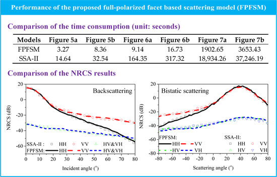
3. Performance of Full-Polarized Facet Based Scattering Model

In this section, the validity of the proposed FPFSM is verified by comparing the NRCS results calculated by the proposed method and the original SSA-II for different radar configurations, incident frequencies, and polarizations. It should be noted that for low grazing angles, the shading effect and the existence of irregular waves (such as breaking waves) have an effect on the NRCS results. The proposed method does not consider these effects because the main purpose of this paper is not to solve the problems at low grazing angles but to propose a facet-based method to investigate the full-polarized EM scattering characteristic of electrically large sea surfaces efficiently. Therefore, the numerical range of the incident angle is 0° to 80° in monostatic configuration, and the scattering angle varies from −80° to 80° in bistatic configuration. In addition, the calculation time and the memory consumption are also compared to show the higher efficiency and much lower memory consumption of FPFSM. Furthermore, the Doppler spectrum results are also shown to further demonstrate its good performance.

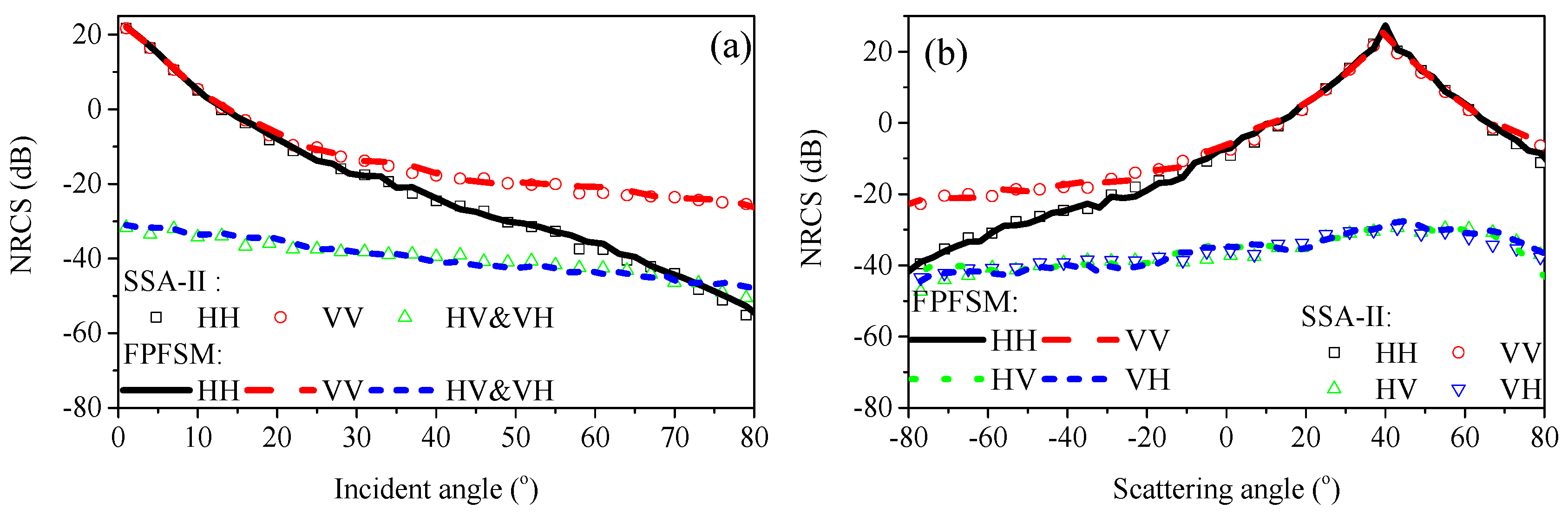
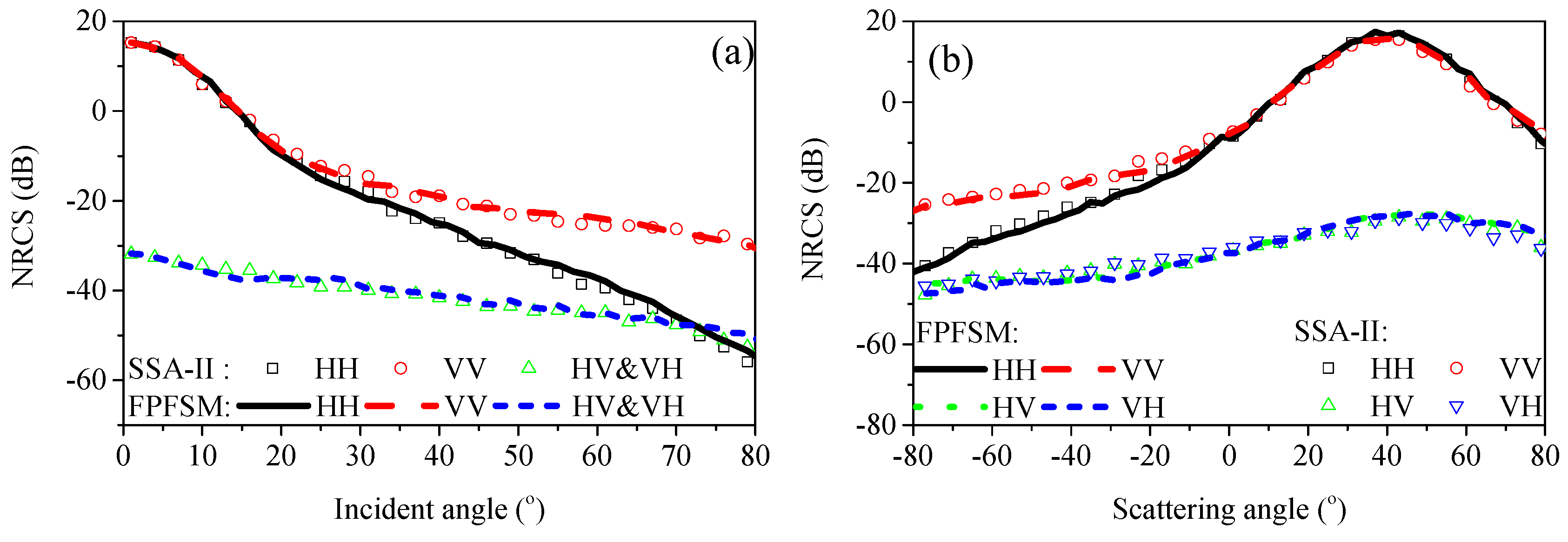
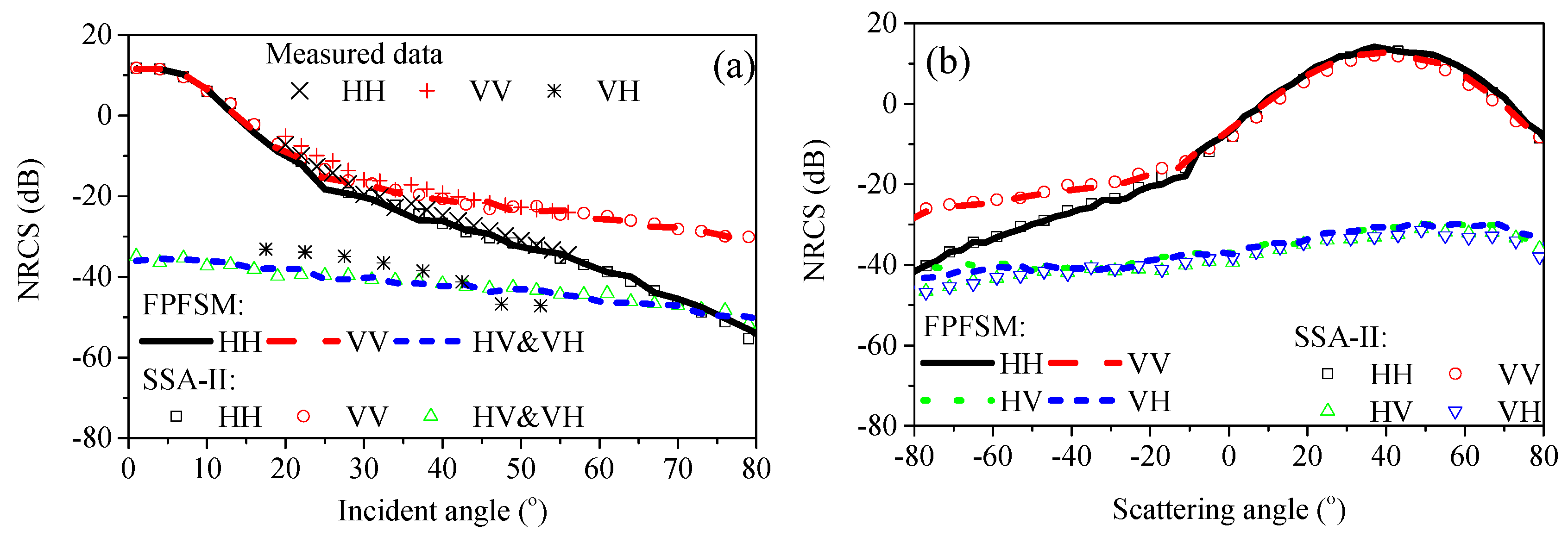
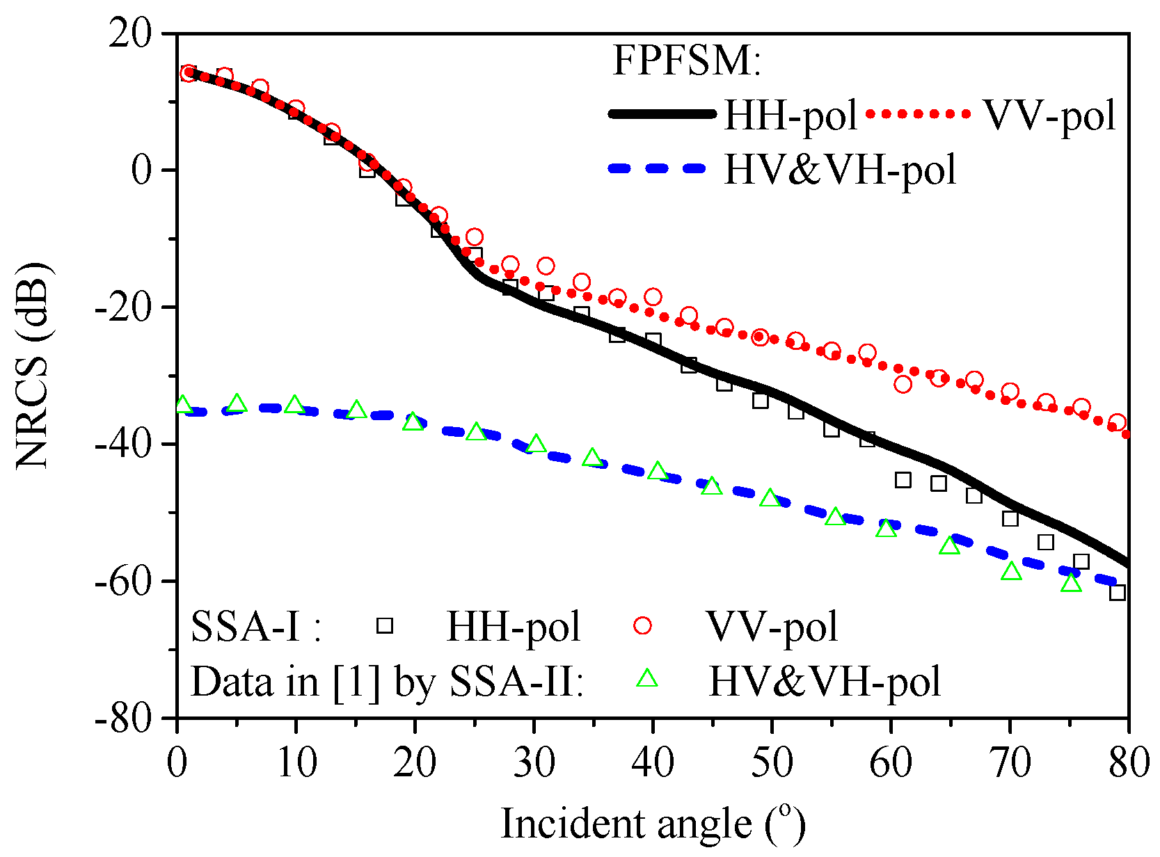
3.1. Normalized Radar Cross Section Results for Different Wave Bands

In this paper, the two-dimensional sea surfaces are all generated using the Elfouhaily spectrum [35] accompanied by Longuet-Higgins’ directional function [36]. First, Figure 4a–c shows the averaged NRCS results calculated by FPFSM with different samples. The tapered incident wave [37] is employed, and the tapering parameter is selected as $L/4$ with L the dimension of the sea surface, the incident frequency is 1 GHz. The size of the sea surface is $40\mathrm{m}\times 40\mathrm{m}$, the wind speed is $u_{10}=5\mathrm{m}/\mathrm{s}$ at 10 m height above the mean sea level in the upwind direction, and the Elfouhaily spectrum as a function of wavenumber for such a wind speed is shown in Figure 4d. It can be observed that the NRCS results from one sample show obvious differences with the averaged results, and the averaged NRCS results tend to be stable for a fixed incident angle with the increasing samples. Thus, the averaged NRCS results from 50 samples are used in this paper to do the comparison with the SSA-II method.

Then, Figure 5, Figure 6 and Figure 7 illustrate the comparisons of NRCS results that calculated by FPFSM and SSA-II at ultra high frequency (UHF) band (300 MHz), L-band (1 GHz), and C-band (8 GHz) for monostatic and bistatic configurations, and the NRCS results are averaged over 50 samples of sea surfaces. The size of the sea surface is $40\mathrm{m}\times 40\mathrm{m}$, the wind speed is $u_{10}=5\mathrm{m}/\mathrm{s}$ in upwind direction. Then in Figure 8, the NRCS results for higher wind speeds ($u_{10}=8\mathrm{m}/\mathrm{s},10\mathrm{m}/\mathrm{s}$) are calculated and compared with the SSA-II as well. The good agreement of the results calculated by the two methods indicates that the good performance of the proposed method.

Moreover, the NRCS results as a function of incident angle at C band are calculated with FPFSM and SSA-II and are compared with real SAR data in Figure 6a. The real SAR data are obtained with the CMOD-5 model [38] for horizontal-transmit–horizontal-receive (HH) polarization mode. Then, one can calculate the vertical-transmit–vertical -receive (VV) polarized results based on the polarization ratio [39]. As for cross-polarized case, the real SAR data are calculated with the cross-polarization geophysical model function for C-band radar backscattering [40]. From the simulated results, we can observe that the co-polarized NRCS results calculated by the FPFSM and the SSA-II agree well with the measured data. However, a discrepancy occurs of about 2~5 dB for the cross-polarization mode. The obvious difference appears in other researches as well the reason for which is the measurement of cross-polarized radar return from the ocean surface is always a challenge due to the weakness of this component [41].

On the other hand, the computation time for calculating the NRCS results in Figure 5, Figure 6 and Figure 7 with one sample of sea surface by the two methods with an angle interval of $1°$ are shown in

Table 1. Comparison of the time consumption (unit: seconds) between FPFSM and SSA-II.

Models	Figure 5a	Figure 5b	Figure 6a	Figure 6b	Figure 7a	Figure 7b
FPFSM	3.27	8.36	9.14	16.73	1902.65	3653.43
SSA-II	14.64	32.54	164.35	317.32	18,934.26	37,246.19

. These results are calculated by central processing unit (CPU) under the configuration: Intel(R) Core(TM) [email protected] GHz. The comparison of the computation time indicates higher computing efficiency of FPFSM compared with SSA-II. In addition, the comparison of the peak memory consumption is given in

Table 2. Comparison of the peak memory consumption (unit: Mb) between FPFSM and SSA-II.

Models	Figure 5a	Figure 6a	Figure 7a
FPFSM (Near specular reflection direction)	23.2	58.9	4129.3
FPFSM (Diffuse scattering direction)	2.7	3.9	167.6
SSA-II	49.3	514.6	31,527.8

. Noting that the memory consumption is the same in monostatic and bistatic configurations for a fixed frequency and surface size, we only show the comparison in monostatic configuration. In addition, for the FPFSM, the detailed implementation methods are not the same for different scattering directions, thus, the consumed memory of FPFSM in the near specular reflection direction and diffuse scattering direction are shown separately. The comparison result indicates that the proposed method saves a significant memory when analysing the scattering characteristic from sea surfaces, which means it is able to be applied to super electrically large sea surfaces.

Moreover, the mean and the maximum errors between the FPFSM and the SSA-II are shown in

Table 3. Mean errors and maximum errors (unit: dB) between FPFSM and SSA-II.

Models		Figure 5a	Figure 5b	Figure 6a	Figure 6b	Figure 7a	Figure 7b
Mean error	HH	1.34	1.51	1.45	1.22	1.19	0.99
	VV	1.10	1.49	1.12	1.02	0.84	0.92
	HV	1.20	1.23	1.26	1.45	0.71	1.93
	VH	1.20	1.19	1.26	1.72	0.71	1.54
Maximum error	HH	2.88	2.81	2.73	2.45	2.53	2.71
	VV	2.53	2.85	2.25	1.93	2.46	2.44
	HV	2.84	2.69	2.12	2.97	2.38	2.78
	VH	2.84	2. 87	2.12	3.06	2.38	2.89

to quantify the goodness of fit between the two methods. The mean error and the maximum error are defined as

$${\Delta }_{\mathrm{mean}}=E\left[\left|{\sigma }_{\mathrm{FPFSM}}\left(\mathrm{dB}\right)-{\sigma }_{\mathrm{SSA}-\mathrm{II}}\left(\mathrm{dB}\right)\right|\right],{\Delta }_{\max }=\max \left[\left|{\sigma }_{\mathrm{FPFSM}}\left(\mathrm{dB}\right)-{\sigma }_{\mathrm{SSA}-\mathrm{II}}\left(\mathrm{dB}\right)\right|\right]$$

(25)

where ${\sigma }_{\mathrm{SSA}-\mathrm{II}}$ is the NRCS results calculated with SSA-II. It is shown that the maximum errors are about 2~3 dB and mean errors are only about 1 dB, which indicates the good performance of FPFSM.

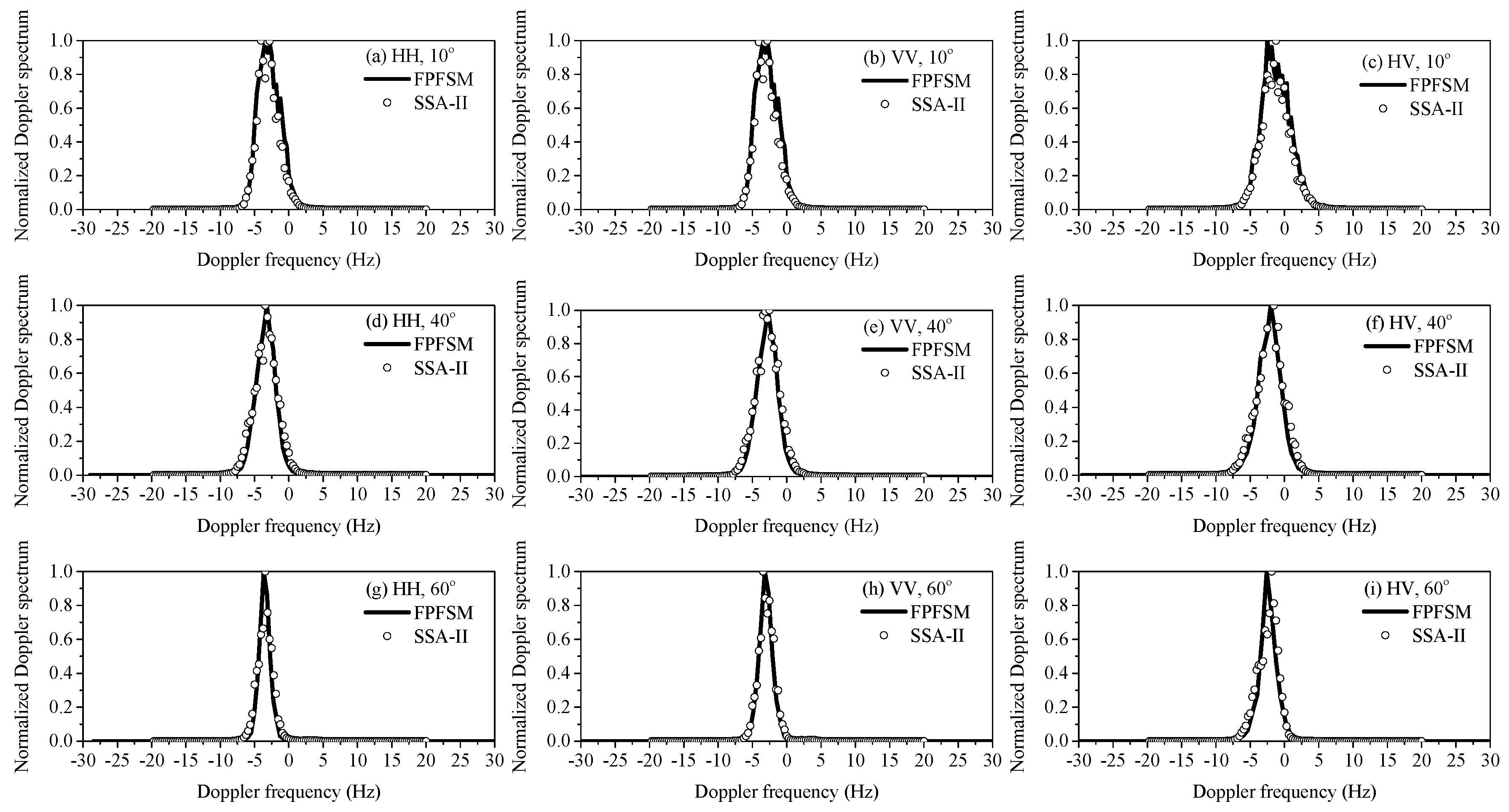
3.2. Comparison of Doppler Spectrum

Apart from the NRCS results, the Doppler spectrum of the sea surface is also of great value to obtain the sea condition information. The Doppler effect is due to the change in frequency of a wave in relation to an observer who is moving relative to the wave source. In regards to the ocean surface, it is caused by the change of the sea surface velocity projected along the line-of-sight of the radar. As two parameters of the Doppler spectrum, the Doppler shift reflects the line-of-sight velocity of the scatterers weighted by their contribution to the backscattered power [42], and the bandwidth of the Doppler spectrum is determined by the variance of the velocity distribution of the scattering facets at the sea surface [43]. In this subsection, the proposed method is used to analyze the Doppler spectrum of the time-varying sea surface at L-band with a standard spectral estimation technique [44,45]. It can be given as

$$S_{\mathrm{Doppler}}=\langle \frac{1}{T}{\left|{\displaystyle \underset{0}{\overset{T}{\int }}{\mathit{E}}_{PQ}^{\mathrm{s}}\left(t\right)\exp \left(\mathrm{j}2\mathsf{\pi }ft\right)\mathrm{d}t}\right|}^2\rangle$$

(26)

where ${\mathit{E}}_{PQ}^{\mathrm{s}}\left(t\right)$ is the scattered field calculated with Equation (21) at time t, the angular bracket $\langle \cdot \rangle$ means the average from different samples of sea surfaces, T is the total evolution time for a time-varying sea surface.

Figure 9 illustrates the normalized Doppler spectrum averaged over 100 samples of sea surfaces for different polarizations and incident angles. In the simulation, the wind speed is 5 m/s in the upwind direction, the time step is set as 0.025 s and the total evolution time is 3.2 s. The size of the sea surface is $50\mathrm{m}\times 50\mathrm{m}$. The frequency of the incident wave is 1 GHz. As indicated in Figure 8, one can observe the good performance of the proposed method on investigating the Doppler spectrum for different radar configurations and polarizations.

4. Analyses of Electromagnetic Scattering Characteristics at Ka-Band

In this section, the FPFSM is further applied to Ka-band (30 GHz). The NRCS results and the Doppler spectrums from sea surfaces at Ka-band are calculated and analyzed by the proposed method.

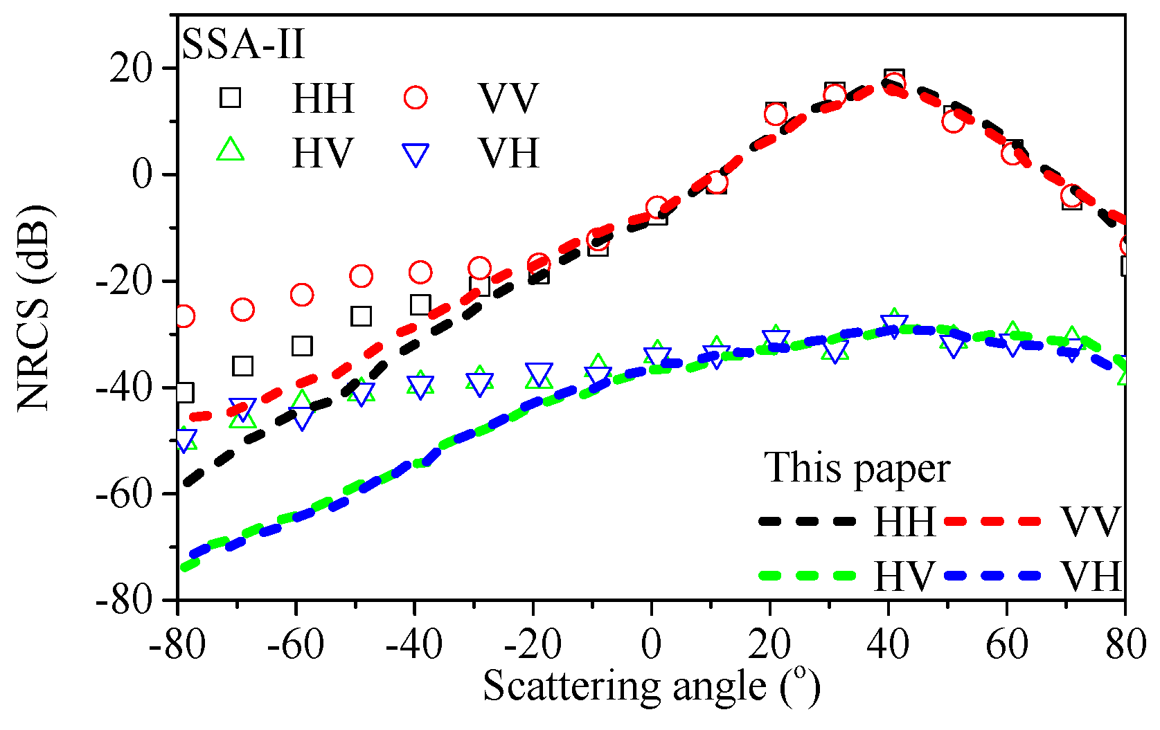
4.1. Normalized Radar Cross Section under Monostatic Configuration

Firstly, the backscattered NRCS results calculated by the FPFSM are given in Figure 10. The size of the sea surface and the wind speed is the same as that in Section 3.1. At Ka-band, the SSA-II is difficult to implement due to the very large requirement for computer memory. Thus, for the comparison, the co-polarized results calculated with FPFSM are compared with those generated by the first order small slope approximation (SSA-I) with the spectral decomposition method [46], and the cross-polarized results are compared with the data in Guérin et al. [1]. From Figure 10, it can be observed that the two models are in good agreement, which indicates the good performance of FPFSM in evaluating the radar returns from the sea surface at higher microwave bands.

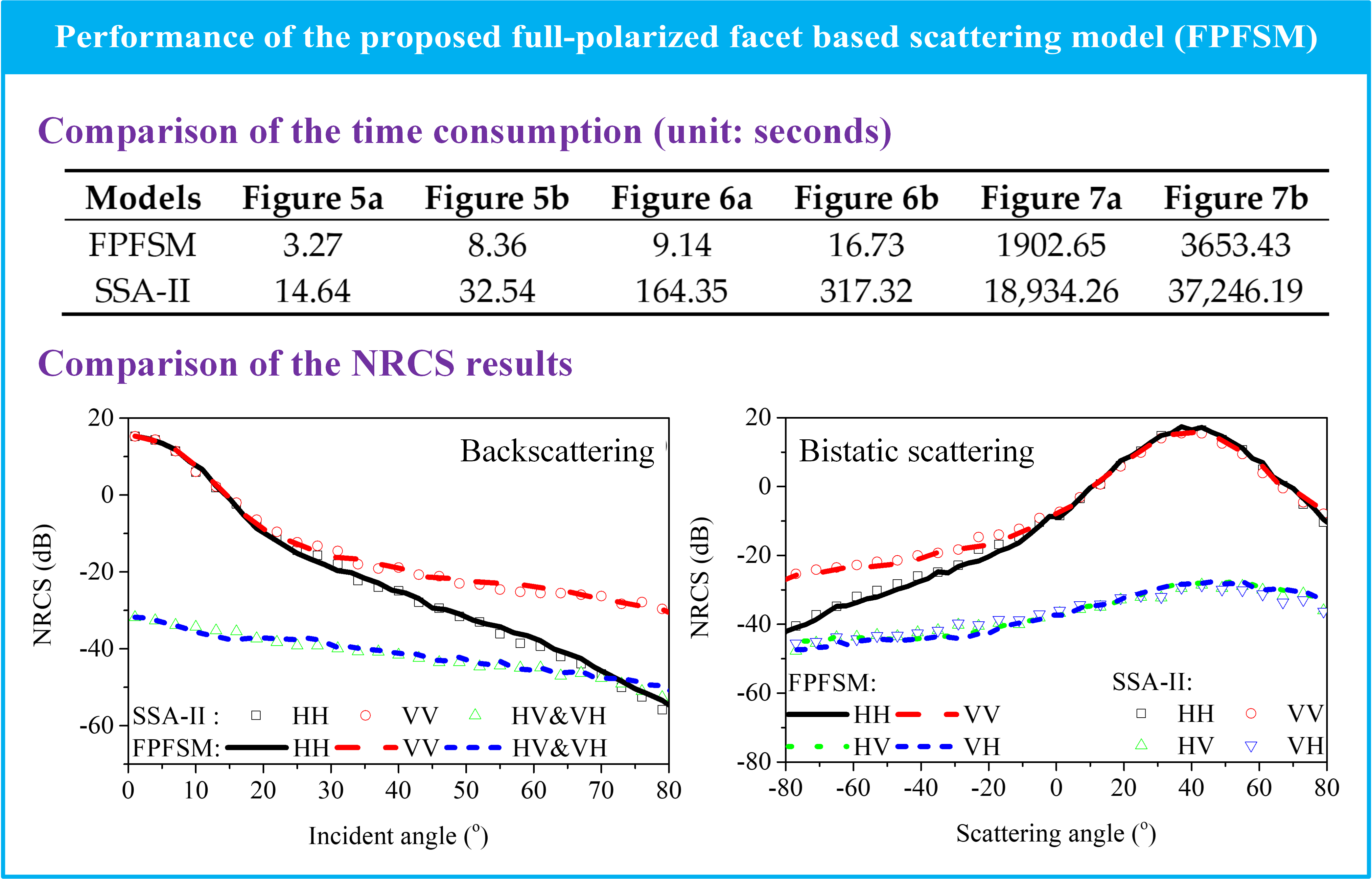
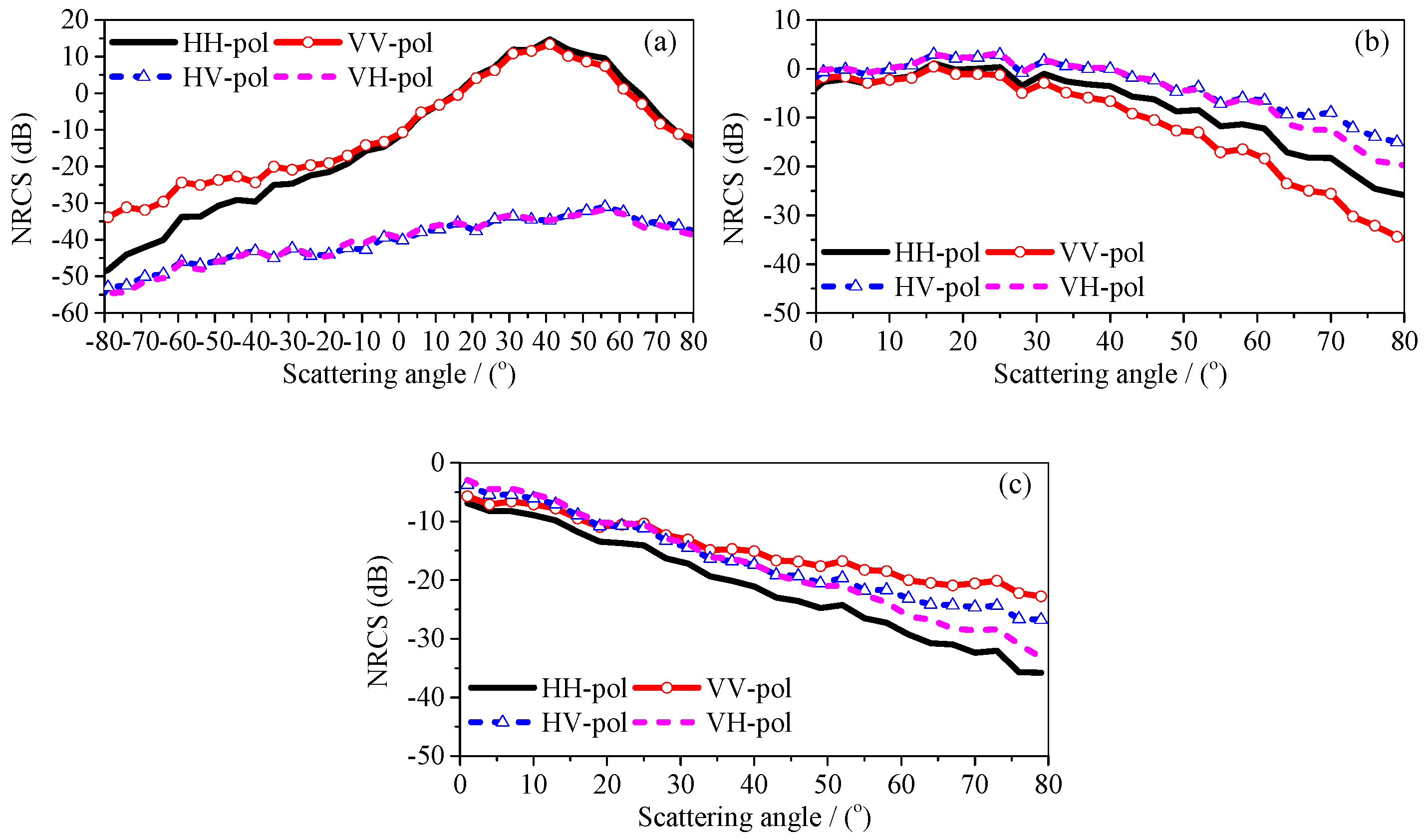
4.2. Normalized Radar Cross Section under Bistatic Configuration

Furthermore, the NRCS results at Ka-band under forward–backward configuration is shown in Figure 11a. Here, the incident angle is ${\theta }_{\mathrm{i}}=40°$, and the scattering angle ${\theta }_{\mathrm{s}}$ varies from $-80°$ to $80°$. Specifically, in this configuration, one can observe that the maximum energy is received around the specular direction for co-polarized cases, which is a logical result. However, for cross-polarized results, the maximum value does not appear in the specular direction. In addition, unlike the backscattering configuration, the NRCS results for vertical-transmit-horizontal-receive (HV) polarization are not exactly the same as the horizontal-transmit-vertical-receive (VH) polarized results except for the specular direction.

Furthermore, the NRCS results in fully bistatic configurations at Ka-band are investigated as well. Figure 11b,c gives the NRCS with the incident direction ${\theta }_{\mathrm{i}}={40}^{\mathrm{o}},{\phi }_{\mathrm{i}}=0^{\mathrm{o}}$ and the scattering direction: (b) ${\theta }_{\mathrm{s}}=-{80}^0~{80}^0,{\phi }_{\mathrm{s}}={45}^{\mathrm{o}}$; (c) ${\theta }_{\mathrm{s}}=-{80}^0~{80}^0,{\phi }_{\mathrm{s}}={135}^{\mathrm{o}}$. It is interesting to find that the discrepancy between the VH and HV polarizations became wider in these configurations. In addition, the levels of cross-polarized NRCS are larger than the co-polarized NRCS in the plane of ${\phi }_{\mathrm{s}}={45}^{\mathrm{o}}$, and the VV-polarized NRCS is the minimum. However, in the plane of ${\phi }_{\mathrm{s}}={135}^{\mathrm{o}}$, the behavior is the opposite. The behaviors of the aforementioned curves show a very good trend with conclusions drawn in other relevant papers [47,48].

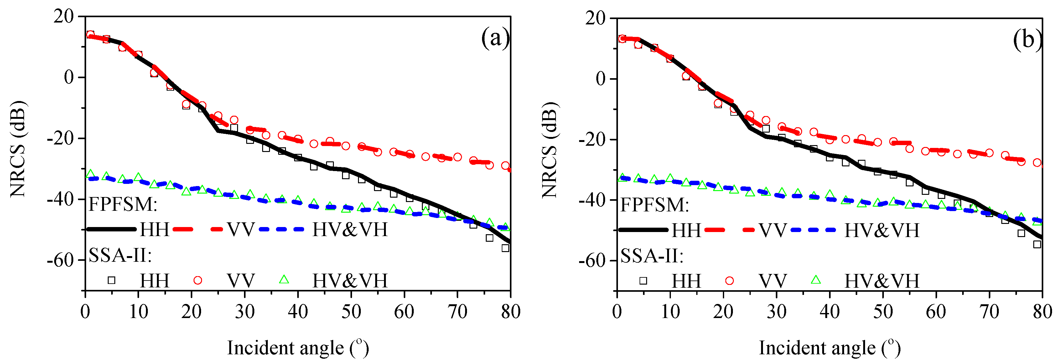
4.3. Normalized Radar Cross Section Dependence on Wind Speed

When referenced to 2D surfaces, it is of great interest to discuss the dependence of NRCS on the wind speed. In Figure 12, NRCS results which vary with wind speed are shown under forward–backward configuration at Ka-band. From Figure 12, several items of importance may be deduced. First, the maximum of energy for co-polarizations is received around the specular direction, which is a logic statement. Second, the magnitude of NRCS for cross-polarizations increases with the increase in wind speed. However, when it comes to the co-polarization modes, the scattering coefficient decreases with wind speed around the specular direction, whereas it increases with wind speed when the scattering direction is away from the specular direction.

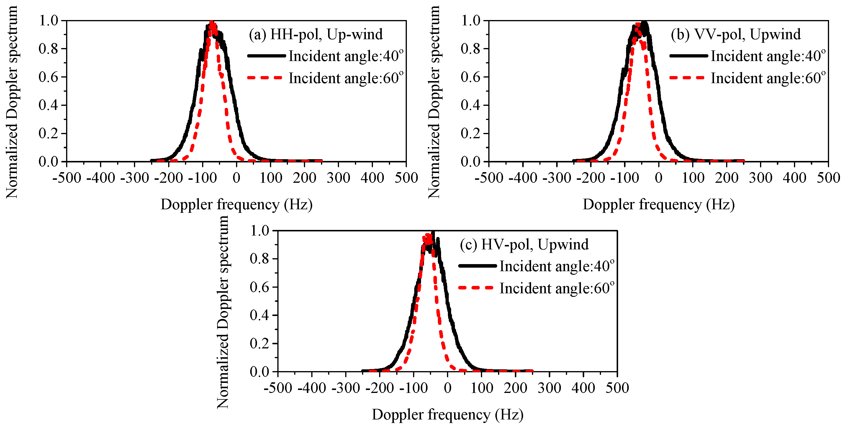
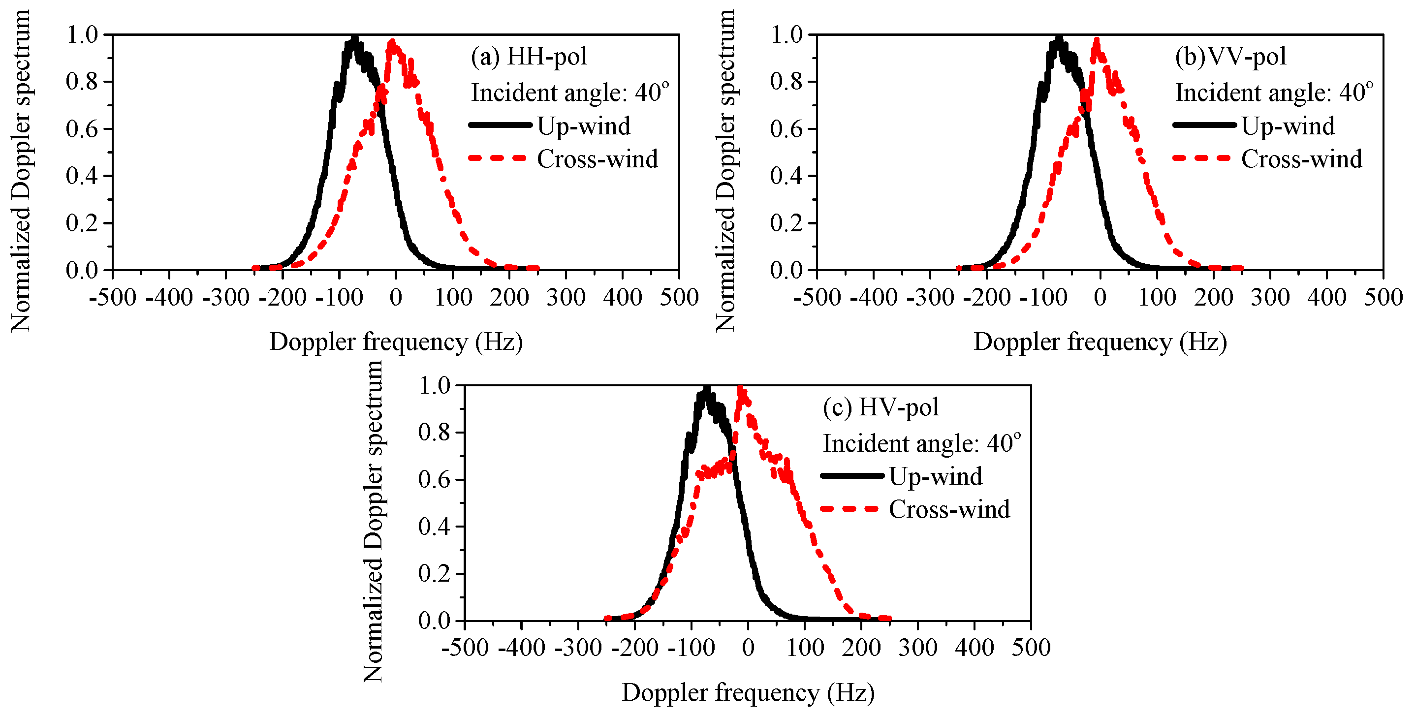
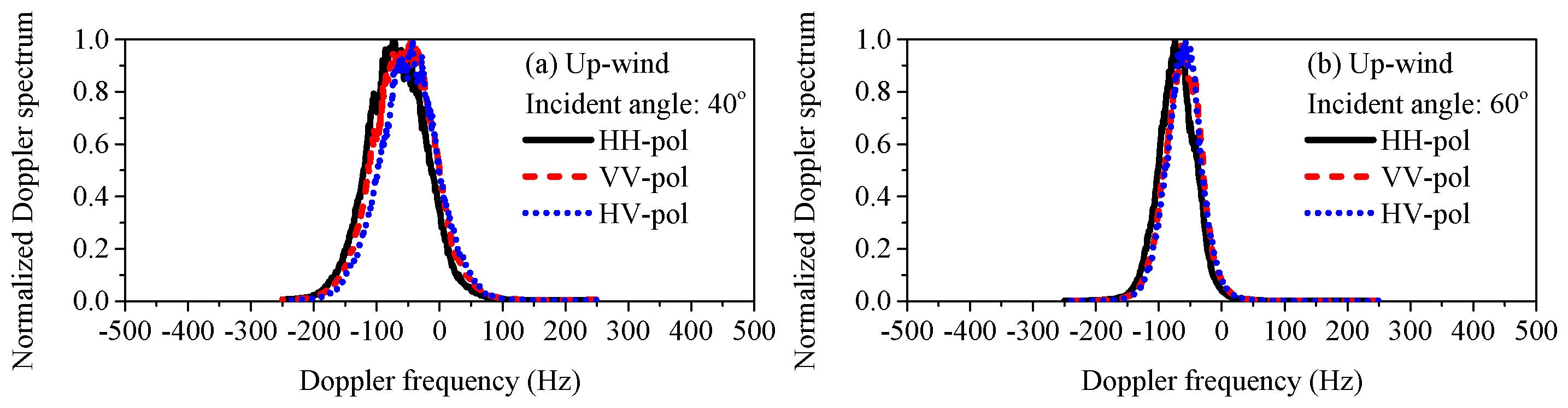
4.4. Doppler Spectrum of Time-Evolving Sea Surfaces

In this part, Doppler spectrum characteristics at Ka-band is analyzed with the standard spectral estimation technique. In the following simulations, the normalized Doppler spectrum are averaged from 100 samples of sea surfaces with the size of $50\mathrm{m}\times 50\mathrm{m}$, and the wind speed of 5 m/s. The time step is set as 0.002 s and the total evolution time is 2.048 s.

Figure 13 compares the Doppler spectrum for up-wind direction with different incident angles. As indicated in Figure 12, it is observed that at moderate incident angles, the Doppler spectrum becomes wider compared with a lower incident angle. However, the variation of Doppler central frequency is not very obvious. In addition, the Doppler spectrum at Ka-band for different wind directions and polarizations are shown in Figure 14. In fact, researches have reported that there are two peaks in the cross-wind direction [5,7,31], which can be attributed to the fact that both the waves moving toward and away from the radar can be detected. However, the two peaks aliased to one peak due to the broader shape of the spectrum for Ka-band.

Figure 15 illustrates the comparison of Doppler spectrum for different polarizations. When the incident angle is $40°$, it is observed that the Doppler shift at HH polarization mode is larger than that at VV polarization mode, and the Doppler shifts at cross polarization modes are the smallest. As for the Doppler width, the discrepancy caused by polarizations are relatively small. For the incident angle of $60°$, the difference of Doppler width between HH and VV polarizations are obvious. However, there is almost no difference for the Doppler spectrum between VV and cross polarizations. That is to say for large incident angles, both the Doppler central frequency and the width are close for VV and HV polarizations.

5. Conclusions

In this paper, FPFSM shows quite a good accuracy and computing efficiency in evaluating the radar returns from the electrically large sea surface, and it works well in a wide range of frequencies. In addition, the scattering characteristics from sea surface are predicted by FPFSM at Ka-band in bistatic configurations as a function of scattering angle, polarization mode, and wind speed. One can draw the following conclusions: (i) The maximum of energy is received around the specular direction in the forward–backward configuration for co-polarizations, but it does not hold true for cross polarizations. (ii) In cross polarization cases, the level of NRCS results increase with wind speed in both specular and diffuse scattering directions, which is different in the co-polarized cases. (iii) As for the Doppler spectrum, the results for different wave bands show similar characteristics in up-wind and co-polarizations cases. However, for cross-wind direction, the Doppler spectrum has two peaks at low wave bands but the two peaks aliased to one at Ka-band. All of the numerical results show the good performance of the proposed method, and it can be further applied to analyze the scattering from targets over sea surfaces and to the SAR imaging simulators, which will benefit the recognition and detection of targets in a maritime environment.

References

1. Guérin, C.A.; Johnson, J.T. A Simplified Formulation for Rough Surface Cross-Polarized Backscattering Under the Second-Order Small-Slope Approximation. IEEE Trans. Geosci. Remote Sens. 2015, 53, 6308–6314. [Google Scholar] [CrossRef] [Green Version]
2. Hwang, P.A.; Perrie, W.; Zhang, B. Cross-Polarization Radar Backscattering from the Ocean Surface and Its Dependence on Wind Velocity. IEEE Geosci. Remote Sens. Lett. 2014, 11, 2188–2192. [Google Scholar] [CrossRef]
3. Schuler, D.L.; Lee, J.S.; Kasilingam, D.; Pottier, E. Measurement of ocean surface slopes and wave spectra using polarimetric SAR image data. Remote Sens. Environ. 2004, 91, 198–211. [Google Scholar] [CrossRef]
4. Xie, L.; Zhang, H.; Wang, C.; Shan, Z. Similarity analysis of entropy/alpha decomposition between HH/VV dual- and quad-polarization SAR data. Remote Sens. Lett. 2015, 6, 228–237. [Google Scholar] [CrossRef]
5. Li, X.F.; Xu, X.J. Scattering and Doppler Spectral Analysis for Two-Dimensional Linear and Nonlinear Sea Surfaces. IEEE Trans. Geosci. Remote Sens. 2010, 49, 603–611. [Google Scholar] [CrossRef]
6. Khenchaf, A. Bistatic Scattering and Depolarization by Randomly Rough Surfaces: Application to the Natural Rough Surfaces in X-band. Waves Random Media 2001, 11, 61–89. [Google Scholar] [CrossRef]
7. Wang, J.N.; Xu, X.J. Doppler Simulation and Analysis for 2-D Sea Surfaces Up to Ku-Band. IEEE Trans. Geosci. Remote Sens. 2015, 54, 466–478. [Google Scholar] [CrossRef]
8. Bass, F.G.; Fuks, I.M.; Kalmyicov, A.I.; Ostrovsky, I.E.; Rosenberg, A.D. Very High Frequency Radiowave Scattering by a Disturbed Sea Surface PART I: Scattering from A Slightly Disturbed Boundary. IEEE Trans. Antennas Propag. 1968, 16, 554–559. [Google Scholar] [CrossRef]
9. Voronovich, A.G. Small-slope approximation for electromagnetic wave scattering at a rough interface of two dielectric half-spaces. Waves Random Media 1994, 4, 337–367. [Google Scholar] [CrossRef]
10. Li, J.X.; Zhang, M.; Fan, W.N.; Nie, D. Facet-Based Investigation on Microwave Backscattering from Sea Surface with Breaking Waves: Sea Spikes and SAR Imaging. IEEE Trans. Geosci. Remote Sens. 2017, 55, 2313–2325. [Google Scholar] [CrossRef]
11. Du, Y.; Yang, X.; Chen, K.-S.; Ma, W.; Li, Z. An Improved Spectrum Model for Sea Surface Radar Backscattering at L-Band. Remote Sens. 2017, 9, 776. [Google Scholar] [CrossRef]
12. Yang, J.S.; Du, Y.; Shi, J.C. Polarimetric simulations of bistatic scattering from perfectly conducting ocean surfaces with 3 m/s wind speed at L band. IEEE J. Sel. Top. Appl. Earth Obs. Remote Sens. 2016, 9, 1176–1186. [Google Scholar] [CrossRef]
13. Reale, F.; Dentale, F.; Carratelli, E.P. Numerical simulation of whitecaps and foam effects on satellite altimeter response. Remote Sens. 2014, 6, 3681–3692. [Google Scholar] [CrossRef]
14. Zheng, H.; Khenchaf, A.; Wang, Y.; Ghanmi, H.; Zhang, Y.; Zhao, C. Sea surface monostatic and bistatic EM scattering using SSA-1 and UAVSAR data: Numerical evaluation and comparison using different sea spectra. Remote Sens. 2018, 10, 1084. [Google Scholar] [CrossRef]
15. Huang, W.; Liu, X.; Gill, E.W. An empirical mode decomposition method for sea surface wind measurements from X-band nautical radar data. IEEE Trans. Geosci. Remote Sens. 2017, 55, 6218–6227. [Google Scholar] [CrossRef]
16. Ji, Q.; Shao, W.; Sheng, Y.; Yuan, X.; Sun, J.; Zhou, W.; Zuo, J. A promising method of typhoon wave retrieval from Gaofen-3 synthetic aperture radar image in VV-polarization. Sensors 2018, 18, 2064. [Google Scholar] [CrossRef] [PubMed]
17. Clarizia, M.P.; Gommenginger, C.; Di, B.M.; Galdi, C.; Srokosz, M.A. Simulation of L-band bistatic returns from the ocean surface: A facet approach with application to ocean GNSS reflectometry. IEEE Trans. Geosci. Remote Sens. 2012, 50, 960–971. [Google Scholar] [CrossRef]
18. Plant, W.J. Microwave Sea Return at Moderate to High Incidence Angles. Waves Random Media 2003, 13, 339–354. [Google Scholar] [CrossRef]
19. West, J.C. Correlation of Bragg scattering from the sea surface at different polarizations. Waves Random Media 2005, 15, 395–403. [Google Scholar] [CrossRef]
20. Franceschetti, G.; Migliaccio, M.; Riccio, D. On Ocean SAR Raw Signal Simulation. IEEE Trans. Geosci. Remote Sens. 1993, 31, 880–884. [Google Scholar] [CrossRef]
21. Li, J.X.; Zhang, M.; Wei, P.B.; Jiang, W.Q. An Improvement on SSA Method for EM Scattering from Electrically Large Rough Sea Surface. IEEE Geosci. Remote Sens. Lett. 2016, 13, 1144–1148. [Google Scholar] [CrossRef]
22. Wei, P.B.; Zhang, M.; Nie, D.; Jiao, Y.C. Improvement of SSA Approach for Numerical Simulation of Sea Surface Scattering at High Microwave Bands. Remote Sens. 2018, 10, 1021. [Google Scholar] [CrossRef]
23. Guérin, C.A.; Saillard, M. On the High-Frequency Limit of the Second-Order Small-Slope Approximation. Waves Random Media 2003, 13, 75–88. [Google Scholar] [CrossRef]
24. Voronovich, A.G.; Zavorotny, V.U. Theoretical model for scattering of radar signals in Ku- and C-bands from a rough sea surface with breaking waves. Waves Random Media 2001, 11, 247–269. [Google Scholar] [CrossRef]
25. Gilbert, M.S.; Johnson, J.T. A study of the higher-order small-slope approximation for scattering from a Gaussian rough surface. Waves Random Media 2003, 13, 137–149. [Google Scholar] [CrossRef]
26. Klein, L.A.; Swift, C.T. An improved model for the dielectric constant of sea water at microwave frequencies. IEEE Trans. Antennas Propag. 1977, 25, 104–111. [Google Scholar] [CrossRef]
27. Voronvich, A.G. A two-scale model from the point of view of the small-slope approximation. Waves Random Media 1996, 66, 73–83. [Google Scholar] [CrossRef]
28. Martin, S. An Introduction to Ocean Remote Sensing; Cambridge University Press: New York, NY, USA, 2011; p. 274. ISBN 9781107019386. [Google Scholar]
29. Meissner, T.; Wentz, F. An updated analysis of the ocean surface wind direction signal in passive microwave brightness temperatures. IEEE Trans. Geosci. Remote Sens. 2002, 40, 1230–1240. [Google Scholar] [CrossRef] [Green Version]
30. Pugliese, C.E.; Dentale, F.; Reale, F. Numerical Pseudo-Random Simulation of SAR Sea and Wind Response. In Proceedings of the SEASAR 2006 (ESA SP-613), Frascati, Italy, 23–26 January 2006. [Google Scholar]
31. Bass, F.G.; Fuks, I.M. Wave Scattering from Statistically Rough Surfaces; Pergamon: Oxford, UK, 1979; ISBN 9781483187754. [Google Scholar]
32. Zhang, M.; Chen, H.; Yin, H.C. Facet-Based Investigation on EM Scattering from Electrically Large Sea Surface with Two-Scale Profiles: Theoretical Model. IEEE Trans. Geosci. Remote Sens. 2011, 49, 1967–1975. [Google Scholar] [CrossRef]
33. Valenzuela, G.R. Theories for the interaction of electromagnetic waves and oceanic waves: A review. Bound.-Layer Meteorol. 1978, 13, 61–85. [Google Scholar] [CrossRef]
34. Wright, J.W. A New Model for Sea Clutter. IEEE Trans. Antennas Propag. 1968, 16, 217–223. [Google Scholar] [CrossRef]
35. Elfouhaily, T.; Chapron, B.; Katarsos, K. A unified directional spectrum for long and short wind-driven waves. J. Geophys. Res. 1997, 102, 15781–15796. [Google Scholar] [CrossRef] [Green Version]
36. Longuet-Higgins, M.S.; Cartwright, D.E.; Smith, N.D. Observations of the directional spectrum of sea waves using the motions of a floatation buoy. In Ocean Wave Spectra; Prentice Hall: Upper Saddle River, NJ, USA, 1963. [Google Scholar]
37. Ye, H.X.; Jin, Y.Q. Parameterization of the tapered incidence wave for numerical simulation of electromagnetic scattering from rough surfaces. IEEE Trans. Antennas Propag. 2005, 53, 1234–1237. [Google Scholar] [CrossRef]
38. Hersbach, H.; Stoffelen, A.; Haan, S.D. An improved C-band scatterometer ocean geophysical model function: CMOD5. J. Geophys. Res. Oceans 2007, 112, 225–237. [Google Scholar] [CrossRef]
39. Hwang, P.A.; Zhang, B.; Toporkov, J.V.; Perrie, W. Comparison of composite Bragg theory and quad-polarization radar backscatter from RADARSAT-2: With applications to wave breaking and high wind retrieval. J. Geophys. Res. 2010, 115, 246–255. [Google Scholar] [CrossRef]
40. Hwang, P.A.; Stoffelen, A.; Van Zadelhoff, G.J.; Perrie, W.; Zhang, B.; Li, H.; Shen, H. Cross-polarization geophysical model function for C-band radar backscattering from the ocean surface and wind speed retrieval. J. Geophys. Res. Oceans 2015, 120, 893–909. [Google Scholar] [CrossRef] [Green Version]
41. Voronovich, A.G.; Zavorotny, V.U. Depolarization of microwave backscattering from a rough sea surface: Modeling with small-slope approximation. In Proceedings of the IEEE International Geoscience and Remote Sensing Symposium, Vancouver, BC, Canada, 24–29 July 2011. [Google Scholar] [CrossRef]
42. Romeiser, R.; Thompson, D.R. Numerical study on the along-track interferometric radar imaging mechanism of oceanic surface currents. IEEE Trans. Geosci. Remote Sens. 2000, 38, 446–458. [Google Scholar] [CrossRef]
43. Wang, Y.; Zhang, Y. Investigation on Doppler shift and bandwidth of backscattered echoes from a composite sea surface. IEEE Trans. Geosci. Remote Sens. 2011, 49, 1071–1081. [Google Scholar] [CrossRef]
44. Toporkov, J.V.; Brown, G.S. Numerical simulations of scattering from time-varying, randomly rough surfaces. IEEE Trans. Geosci. Remote Sens. 2000, 38, 1616–1625. [Google Scholar] [CrossRef]
45. Papoulis, A.; Pillai, S.U. Probability, Random Variables, and Stochastic Processes; McGraw-Hill: Boston, MA, USA, 2002; ISBN 9780071226615. [Google Scholar]
46. Jiang, W.Q.; Zhang, M.; Wei, P.B.; Nie, D. Spectral Decomposition Modeling Method and Its Application to EM Scattering Calculation of Large Rough Surface with SSA Method. IEEE J. Sel. Top. Appl. Earth Obs. Remote Sens. 2015, 8, 1848–1854. [Google Scholar] [CrossRef]
47. Andreas, A.B.; Khenchaf, A.; Martin, A. Bistatic Radar Imaging of the Marine Environment Part I: Theoretical Background. IEEE Trans. Geosci. Remote Sens. 2007, 45, 3372–3383. [Google Scholar] [CrossRef]
48. Awada, A.; Ayari, M.Y.; Khenchaf, A.; Coatanhay, A. Bistatic scattering from an anisotropic sea surface: Numerical comparison between the first-order SSA and the TSM models. Wave Random Complex Media 2006, 16, 383–394. [Google Scholar] [CrossRef]
Figure 1. Comparison of normalized radar cross sections (NRCS) results between the proposed method and the original second order small slope approximation (SSA-II) method under monostatic configuration in near specular direction. (a) horizontal-transmit-horizontal-receive (HH) polarization; (b) vertical-transmit-vertical-receive (VV) polarization; (c) vertical-transmit-horizontal-receive (HV) polarization.
Remotesensing 11 00075 g001
Figure 2. Comparison of NRCS results between the proposed method and the original SSA-II method under bistatic configuration in the near specular regime.
Remotesensing 11 00075 g002
Figure 3. The global and local coordinates on a facet.
Remotesensing 11 00075 g003
Figure 4. The NRCS results calculated by full-polarized facet based scattering model (FPFSM) with different samples for u 10 = 5   m / s and the Elfouhaily spectrum as a function of the wavenumber. (a) NRCS results at HH polarization mode; (b) NRCS results at VV polarization mode; (c) NRCS results at HV and horizontal-transmit-vertical-receive (VH) polarization modes; (d) Elfouhaily spectrum.
Remotesensing 11 00075 g004aRemotesensing 11 00075 g004b
Figure 5. Comparison of the NRCS results calculated by FPFSM and SSA-II at ultra high frequency (UHF) band. (a) Monostatic configuration; (b) Forward–backward configuration.
Remotesensing 11 00075 g005
Figure 6. Comparison of the NRCS results calculated by FPFSM and SSA-II at L-band. (a) Monostatic configuration; (b) Forward–backward configuration.
Remotesensing 11 00075 g006
Figure 7. Comparison of the NRCS results calculated by FPFSM, SSA-II and real SAR data at C-band. (a) Monostatic configuration; (b) Forward–backward configuration.
Remotesensing 11 00075 g007
Figure 8. Comparison of the NRCS results calculated by FPFSM and SSA-II at L-band with different wind speeds. (a) The wind speed is 8 m/s; (b) The wind speed is 10 m/s.
Remotesensing 11 00075 g008
Figure 9. Comparison of Doppler spectrum results calculated by FPFSM and SSA-II at L-band for different incident angles and polarizations.
Remotesensing 11 00075 g009
Figure 10. Performance of the FPFSM at Ka-band.
Remotesensing 11 00075 g010
Figure 11. Bistatic NRCS evaluated by FPFSM on the variation of scattering angles. (a) θ i = θ s , φ i = 0 ° , φ s = 180 ° ; (b) θ i = 40 ° , φ i = 0 ° , φ s = 45 ° ; (c) θ i = 40 ° , φ i = 0 ° , φ s = 135 ° .
Remotesensing 11 00075 g011
Figure 12. Variation of Bistatic NRCS with wind speeds evaluated by FPFSM for different polarization states. (a) HH and HV polarizations. (b) VV and VH polarizations.
Remotesensing 11 00075 g012
Figure 13. Comparison of Doppler spectrum at Ka-band for different incident angles and polarizations. (a) HH polarization; (b) VV polarization; (c) HV polarization.
Remotesensing 11 00075 g013
Figure 14. Comparison of Doppler spectrum at Ka-band for different wind directions and polarizations. (a) HH polarization; (b) VV polarization; (c) HV polarization.
Remotesensing 11 00075 g014
Figure 15. Comparison of Doppler spectrum at Ka-band for different polarizations and incident angles. (a) Incident angle 40 ° ; (b) Incident angle 60 ° .
Remotesensing 11 00075 g015