A Hybrid GIS Multi-Criteria Decision-Making Method for Flood Susceptibility Mapping at Shangyou, China

 ,
,  ,
,  ,
, 
 , ,
, ,  ,
,  and
and
Abstract
1. Introduction
2. Study Area and Data
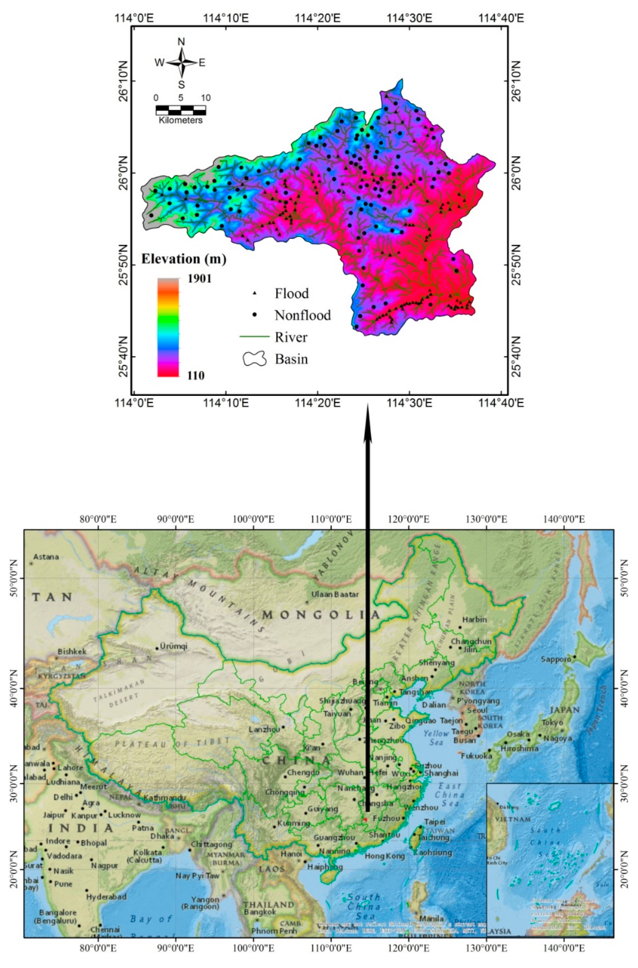
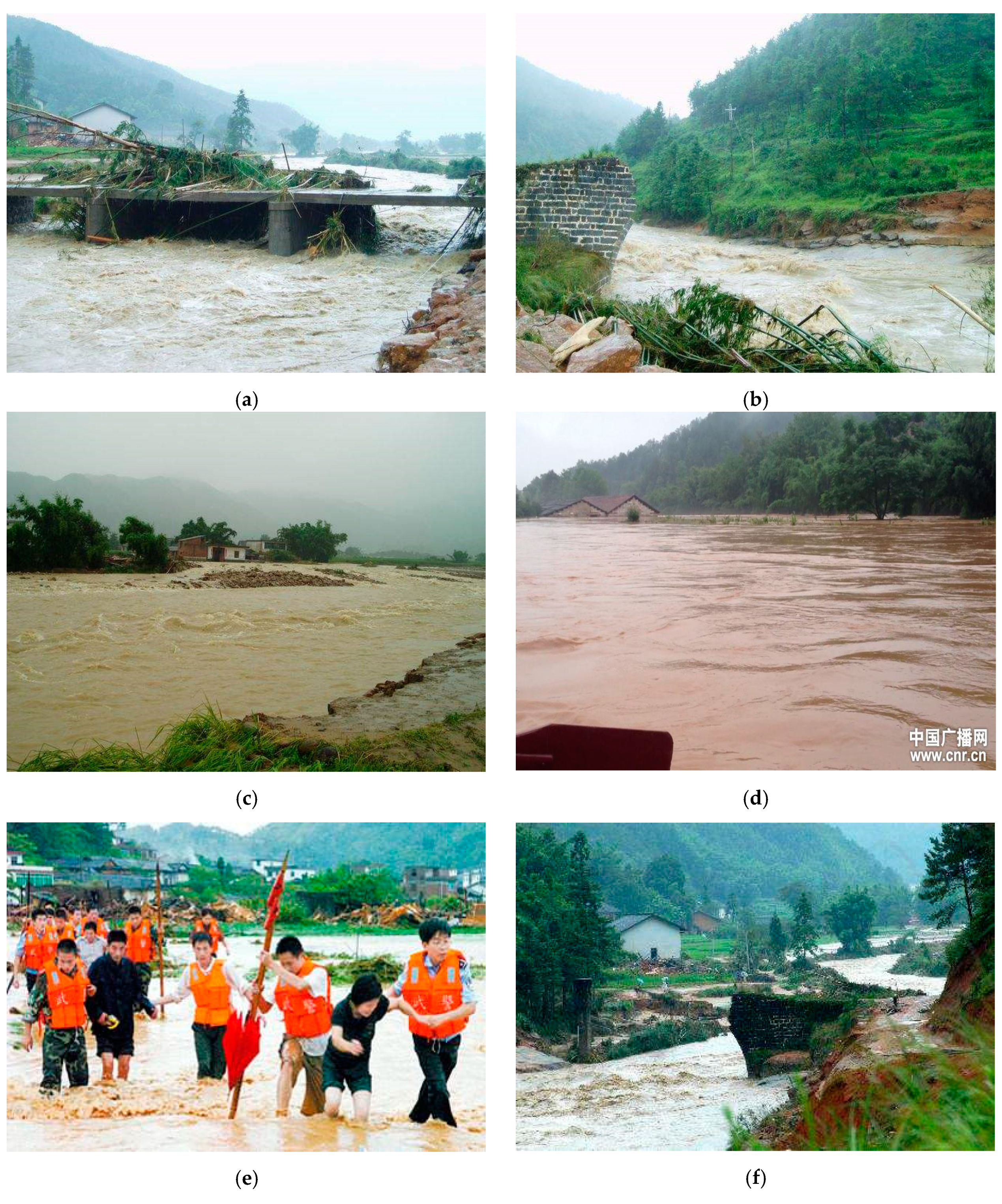
2.1. Description of Study Area
2.2. Available Data
3. Methodology
3.1. Methodological Background
3.2. IRN-DEMATEL-ANP Method
3.2.1. DEMATEL Method
3.2.2. IRN Method
3.2.3. IRN-DEMATEL Method
| Algorithm 1: IRN-DEMATEL |
| Input: The expert pairwise comparison matrices Z Output: CER diagram |
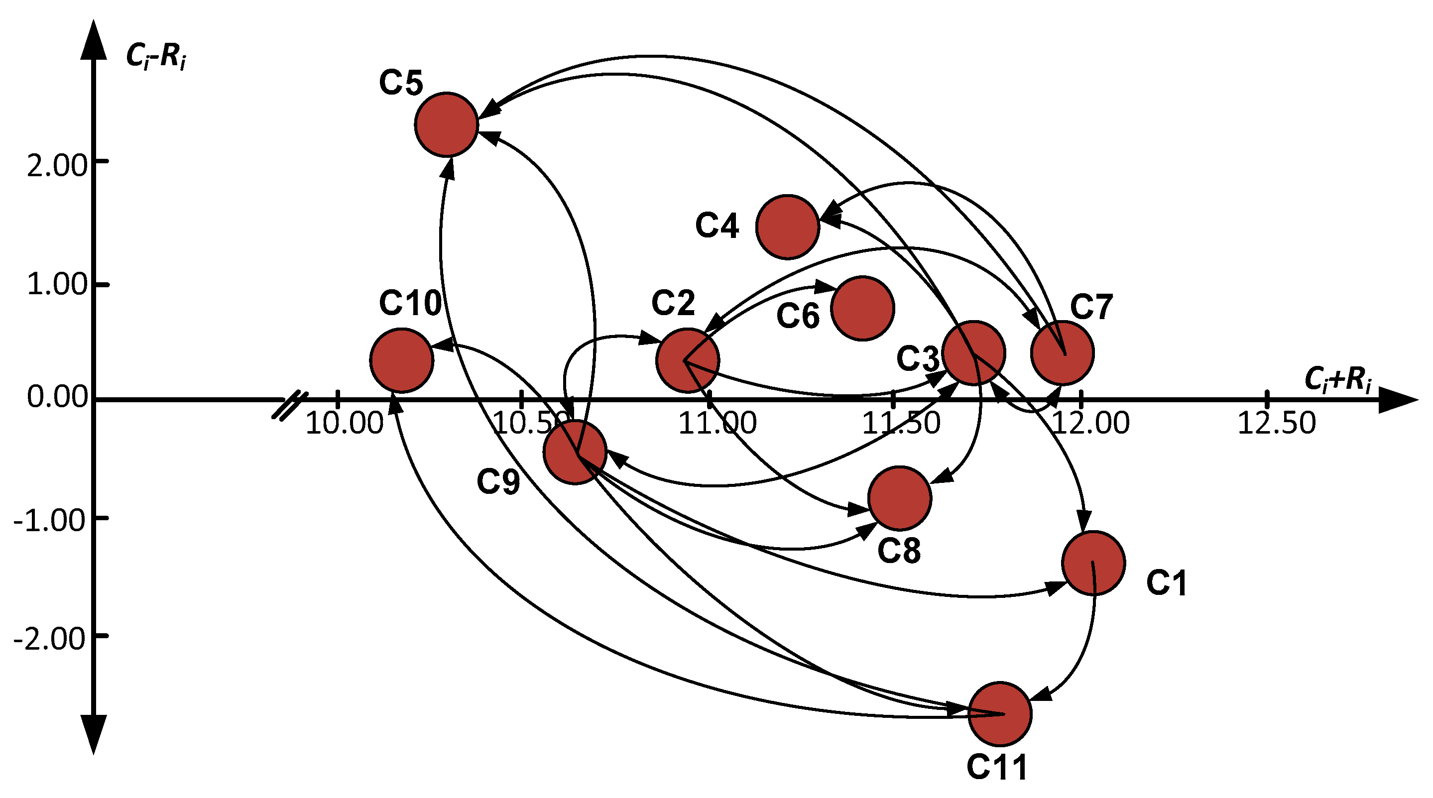
| Step 1: Analysis of factors by experts. Step 2: Calculation of the average matrix . Step 3: A normalized initial direct-relationship matrix can be obtained based on the average matrix Z. Step 4: The total-relationship matrix . Step 5: Calculate the sums of the rows Ri and columns Cj of the total-relationship matrix T [35]. Step 6: Set a threshold value (α) and construct a CER diagram. |
3.2.4. IRN-DEMATEL-ANP Method
| Algorithm 2: IRN-DEMATEL-ANP |
| Input: Total-relation matrix T Output: Weighted super matrix Wα |
| Step 1: Develop an unweighted super matrix. Step 2: Create a normalized total-influence matrix for criteria Tcα., which Tcα is the normalized matrix of T Step 3: Calculating the elements of the unweighted super matrix W, which is the transpose of Tcα. Step 4: Develop a weighted normalized super matrix Wα, which is TDα multiplication by W. The weighted normalized super matrix Wα can be calculated by the normalized influence matrix T with respect to the perspectives. TDα is the result of Tcα divided by dimension. Step 5: Find the limit of the weighted super matrix Wα, which multiply the weighted super matrix by itself multiple times results in the limit super matrix. The weight of each evaluation criterion is solved. |
4. Results
4.1. Conditioning Factor Selection
4.2. MCDA-GIS Evaluation
| Expert 1 rough sequence for C2-C3 | |
| Expert 2 rough sequence for C2-C3 | |
| … | … |
| … | |
| Expert 6 rough sequence for C2-C3 | |
| Expert 1 rough sequence for C2-C3 | |
| Expert 2 rough sequence for C2-C3 | |
| … | … |
| … | |
| Expert 6 rough sequence for C2-C3 | |
| Expert 1 IRN for C2-C3 | , |
| Expert 2 IRN for C2-C3 | , |
| … | … |
| … | |
| Expert 6 IRN for C2-C3 | , |
4.3. Aggregation of Weighted Linear Combinations
4.4. Model Validation
5. Discussions
6. Conclusions
Author Contributions
Funding
Acknowledgments
Conflicts of Interest
References
- Arnell, N.W.; Gosling, S.N. The impacts of climate change on river flood risk at the global scale. Clim. Chang. 2016, 134, 387–401. [Google Scholar] [CrossRef]
- Booij, M.J. Impact of climate change on river flooding assessed with different spatial model resolutions. J. Hydrol. 2005, 303, 176–198. [Google Scholar] [CrossRef]
- Prudhomme, C.; Wilby, R.L.; Crooks, S.; Kay, A.L.; Reynard, N.S. Scenario-neutral approach to climate change impact studies: Application to flood risk. J. Hydrol. 2010, 390, 198–209. [Google Scholar] [CrossRef]
- Næss, L.O.; Bang, G.; Eriksen, S.; Vevatne, J. Institutional adaptation to climate change: Flood responses at the municipal level in norway. Sci. Tech. 2005, 15, 125–138. [Google Scholar] [CrossRef]
- Kay, A.L.; Davies, H.N.; Bell, V.A.; Jones, R.G. Comparison of uncertainty sources for climate change impacts: Flood frequency in england. Clim. Chang. 2009, 92, 41–63. [Google Scholar] [CrossRef]
- Hirabayashi, Y.; Mahendran, R.; Koirala, S.; Konoshima, L.; Dai, Y.; Watanabe, S.; Kim, H.; Kanae, S. Global flood risk under climate change. Nat. Clim. Chang. 2013, 3, 816–821. [Google Scholar] [CrossRef]
- Spence, A.; Poortinga, W.; Butler, C.; Pidgeon, N.F. Perceptions of climate change and willingness to save energy related to flood experience. Nat. Clim. Chang. 2011, 1, 46–49. [Google Scholar] [CrossRef]
- Sampson, C.C.; Smith, A.M.; Bates, P.D.; Neal, J.C.; Alfieri, L.; Freer, J.E. A high-resolution global flood hazard model. Water Resour. Res. 2015, 51, 7358–7381. [Google Scholar] [CrossRef]
- Rojas, R.; Feyen, L.; Bianchi, A.; Dosio, A. Assessment of future flood hazard in europe using a large ensemble of bias-corrected regional climate simulations. J. Geophys. Res. Atmos 2012, 117. [Google Scholar]
- Emerton, R.; Cloke, H.; Stephens, E.; Zsoter, E.; Woolnough, S.; Pappenberger, F. Complex picture for likelihood of enso-driven flood hazard. Nat. Commun. 2017, 8, 14796. [Google Scholar] [CrossRef]
- Wu, S.-J.; Lien, H.-C.; Chang, C.-H. Modeling risk analysis for forecasting peak discharge during flooding prevention and warning operation. Stoch. Environ. Res. Risk Assess. 2010, 24, 1175–1191. [Google Scholar] [CrossRef]
- Wang, Y.; Li, Z.; Tang, Z.; Zeng, G. A gis-based spatial multi-criteria approach for flood risk assessment in the dongting lake region, hunan, central china. Water Resour. Manag. 2011, 25, 3465–3484. [Google Scholar] [CrossRef]
- Bout, B.; Jetten, V. The validity of flow approximations when simulating catchment-integrated flash floods. J. Hydrol. 2018, 556, 674–688. [Google Scholar] [CrossRef]
- Huang, X.; Tan, H.; Zhou, J.; Yang, T.; Benjamin, A.; Wen, S.W.; Li, S.; Liu, A.; Li, X.; Fen, S. Flood hazard in hunan province of china: An economic loss analysis. Nat. Hazards 2008, 47, 65–73. [Google Scholar] [CrossRef]
- Youssef, A.M.; Pradhan, B.; Sefry, S.A. Flash flood susceptibility assessment in jeddah city (kingdom of saudi arabia) using bivariate and multivariate statistical models. Environ. Earth Sci. 2016, 75, 12. [Google Scholar] [CrossRef]
- Hong, H.; Panahi, M.; Shirzadi, A.; Ma, T.; Liu, J.; Zhu, A.X.; Chen, W.; Kougias, I.; Kazakis, N. Flood susceptibility assessment in hengfeng area coupling adaptive neuro-fuzzy inference system with genetic algorithm and differential evolution. Sci. Total Environ. 2018, 621, 1124–1141. [Google Scholar] [CrossRef]
- Hong, H.; Tsangaratos, P.; Ilia, I.; Liu, J.; Zhu, A.X.; Chen, W. Application of fuzzy weight of evidence and data mining techniques in construction of flood susceptibility map of poyang county, China. Sci. Total Environ. 2018, 625, 575–588. [Google Scholar] [CrossRef]
- Bahremand, A.; De Smedt, F.; Corluy, J.; Liu, Y.; Poorova, J.; Velcicka, L.; Kunikova, E. Wetspa model application for assessing reforestation impacts on floods in margecany–hornad watershed, slovakia. Water Resour. Manag. 2007, 21, 1373–1391. [Google Scholar] [CrossRef]
- Oeurng, C.; Sauvage, S.; Sánchez-Pérez, J.-M. Assessment of hydrology, sediment and particulate organic carbon yield in a large agricultural catchment using the swat model. J. Hydrol. 2011, 401, 145–153. [Google Scholar] [CrossRef]
- Costabile, P.; Costanzo, C.; Macchione, F. A storm event watershed model for surface runoff based on 2d fully dynamic wave equations. Hydrol. Process. 2013, 27, 554–569. [Google Scholar] [CrossRef]
- Schumann, G.J.-P.; Andreadis, K.M.; Bates, P.D. Downscaling coarse grid hydrodynamic model simulations over large domains. J. Hydrol. 2014, 508, 289–298. [Google Scholar] [CrossRef]
- Rousseau, M.; Cerdan, O.; Delestre, O.; Dupros, F.; James, F.; Cordier, S. Overland flow modeling with the shallow water equations using a well-balanced numerical scheme: Better predictions or just more complexity. J. Hydrol. Eng. 2015, 20, 04015012. [Google Scholar] [CrossRef]
- Xia, X.; Liang, Q.; Ming, X.; Hou, J. An efficient and stable hydrodynamic model with novel source term discretization schemes for overland flow and flood simulations. Water Resour. Res. 2017, 53, 3730–3759. [Google Scholar] [CrossRef]
- Tehrany, M.S.; Pradhan, B.; Jebur, M.N. Flood susceptibility mapping using a novel ensemble weights-of-evidence and support vector machine models in gis. J. Hydrol. 2014, 512, 332–343. [Google Scholar] [CrossRef]
- Tehrany, M.S.; Lee, M.J.; Pradhan, B.; Jebur, M.N.; Lee, S. Flood susceptibility mapping using integrated bivariate and multivariate statistical models. Environ. Earth Sci. 2014, 72, 4001–4015. [Google Scholar] [CrossRef]
- Kazakis, N.; Kougias, I.; Patsialis, T. Assessment of flood hazard areas at a regional scale using an index-based approach and analytical hierarchy process: Application in rhodope-evros region, greece. Sci. Total Environ. 2015, 538, 555–563. [Google Scholar] [CrossRef] [PubMed]
- Tehrany, M.S.; Pradhan, B.; Jebur, M.N. Flood susceptibility analysis and its verification using a novel ensemble support vector machine and frequency ratio method. Stoch. Environ. Res. Risk Assess. 2015, 29, 1149–1165. [Google Scholar] [CrossRef]
- Rahmati, O.; Pourghasemi, H.R.; Zeinivand, H. Flood susceptibility mapping using frequency ratio and weights-of-evidence models in the golastan province, iran. Geocarto Int. 2016, 31, 42–70. [Google Scholar] [CrossRef]
- Campolo, M.; Soldati, A.; Andreussi, P. Artificial neural network approach to flood forecasting in the river arno. Hydrolog. Sci. J. 2003, 48, 381–398. [Google Scholar] [CrossRef]
- Kia, M.B.; Pirasteh, S.; Pradhan, B.; Wan, N.A.S.; Moradi, A. An artificial neural network model for flood simulation using gis: Johor river basin, malaysia. Environ. Earth Sci. 2012, 67, 251–264. [Google Scholar] [CrossRef]
- Tehrany, M.S.; Pradhan, B.; Jebur, M.N. Spatial prediction of flood susceptible areas using rule based decision tree (dt) and a novel ensemble bivariate and multivariate statistical models in gis. J. Hydrol. 2013, 504, 69–79. [Google Scholar] [CrossRef]
- Mojaddadi, H.; Pradhan, B.; Nampak, H.; Ahmad, N.; Ghazali, A.H.b. Ensemble machine-learning-based geospatial approach for flood risk assessment using multi-sensor remote-sensing data and gis. Geomat. Nat. Hazards Risk 2017, 8, 1080–1102. [Google Scholar] [CrossRef]
- Hammond, M.J.; Chen, A.S.; Djordjević, S.; Butler, D.; Mark, O. Urban flood impact assessment: A state-of-the-art review. Urban Water J. 2015, 12, 14–29. [Google Scholar] [CrossRef]
- Meyer, V.; Scheuer, S.; Haase, D. A multicriteria approach for flood risk mapping exemplified at the mulde river, germany. Nat. Hazards 2009, 48, 17–39. [Google Scholar] [CrossRef]
- Pamučar, D.; Ćirović, G. The selection of transport and handling resources in logistics centers using multi-attributive border approximation area comparison (mabac). Expert Syst. Appl. 2015, 42, 3016–3028. [Google Scholar] [CrossRef]
- Sowmya, K.; John, C.; Shrivasthava, N. Urban flood vulnerability zoning of cochin city, southwest coast of india, using remote sensing and gis. Nat. Hazards 2015, 75, 1271–1286. [Google Scholar] [CrossRef]
- Liu, Z.; Wang, W.; Jin, Q. Manifold alignment using discrete surface ricci flow. CAAI Trans. Intell. Technol. 2016, 1, 285–292. [Google Scholar] [CrossRef]
- Gigovi´C, L.G.C.; Pamučar, D.; Baji´C, Z.B.C.; Drobnjak, S. Application of gis-interval rough ahp methodology for flood hazard mapping in urban areas. Water 2017, 9, 360. [Google Scholar] [CrossRef]
- Chaabani, C.; Chini, M.; Abdelfattah, R.; Hostache, R.; Chokmani, K. Flood mapping in a complex environment using bistatic tandem-x/terrasar-x insar coherence. Remote Sens. 2018, 10, 1873. [Google Scholar] [CrossRef]
- Malczewski, J. GIS and Multicriteria Decision Analysis; John Wiley & Sons: Hoboken, NJ, USA, 1999. [Google Scholar]
- Bathrellos, G.; Skilodimou, H.; Soukis, K.; Koskeridou, E. Temporal and spatial analysis of flood occurrences in the drainage basin of pinios river (thessaly, central greece). Land 2018, 7, 106. [Google Scholar] [CrossRef]
- Chatterjee, K.; Pamucar, D.; Zavadskas, E.K. Evaluating the performance of suppliers based on using the r’amatel-mairca method for green supply chain implementation in electronics industry. J. Clean. Prod. 2018, 184, 101–129. [Google Scholar] [CrossRef]
- Pamučar, D.; Stević, Ž.; Sremac, S. A new model for determining weight coefficients of criteria in mcdm models: Full consistency method (fucom). Symmetry 2018, 10, 393. [Google Scholar] [CrossRef]
- Rijal, S.; Rimal, B.; Sloan, S. Flood hazard mapping of a rapidly urbanizing city in the foothills (birendranagar, surkhet) of nepal. Land 2018, 7, 60. [Google Scholar] [CrossRef]
- Zazo, S.; Rodríguez-Gonzálvez, P.; Molina, J.-L.; González-Aguilera, D.; Agudelo-Ruiz, C.; Hernández-López, D. Flood hazard assessment supported by reduced cost aerial precision photogrammetry. Remote Sens. 2018, 10, 1566. [Google Scholar] [CrossRef]
- Chen, W.; Pourghasemi, H.R.; Panahi, M.; Kornejady, A.; Wang, J.; Xie, X.; Cao, S. Spatial prediction of landslide susceptibility using an adaptive neuro-fuzzy inference system combined with frequency ratio, generalized additive model, and support vector machine techniques. Geomorphology 2017, 297, 69–85. [Google Scholar] [CrossRef]
- Chen, W.; Xie, X.; Peng, J.; Wang, J.; Duan, Z.; Hong, H. Gis-based landslide susceptibility modelling: A comparative assessment of kernel logistic regression, naïve-bayes tree, and alternating decision tree models. Geomat. Nat. Hazards Risk 2017, 8, 950–973. [Google Scholar] [CrossRef]
- Sharifi, M.A. Site selection for waste disposal through spatial multiple criteria decision analysis. J. Telecommun. Inf. Technol. 2004, 3, 1–11. [Google Scholar]
- Geneletti, D.; Beinat, E.; Chung, C.F.; Fabbri, A.G.; Scholten, H.J. Accounting for uncertainty factors in biodiversity impact assessment: Lessons from a case study. Environ. Impact Asses. 2003, 23, 471–487. [Google Scholar] [CrossRef]
- Wu, W.W.; Lee, Y.T. Developing global managers’ competencies using the fuzzy dematel method. Expert Syst. Appl. 2007, 32, 499–507. [Google Scholar] [CrossRef]
- Fontela, E.; Gabus, A. The dematel observer, battelle geneva research center, geneva, switzerland. DOI 1976, 10, 0016–3287. [Google Scholar]
- Gigović, L.; Pamučar, D.; Božanić, D.; Ljubojević, S. Application of the gis-danp-mabac multi-criteria model for selecting the location of wind farms: A case study of vojvodina, serbia. Renew. Energ. 2017, 103, 501–521. [Google Scholar] [CrossRef]
- Pamučar, D.; Mihajlović, M.; Obradović, R.; Atanasković, P. Novel approach to group multi-criteria decision making based on interval rough numbers: Hybrid dematel-anp-mairca model. Expert Syst. Appl. 2017, 88, 58–80. [Google Scholar] [CrossRef]
- Zhai, L.Y.; Khoo, L.P.; Zhong, Z.W. A rough set enhanced fuzzy approach to quality function deployment. Int. J. Adv. Manuf. Technol. 2008, 37, 613–624. [Google Scholar] [CrossRef]
- Song, W.; Ming, X.; Han, Y.; Wu, Z. A rough set approach for evaluating vague customer requirement of industrial product-service system. Int. J. Prod. Res. 2013, 51, 6681–6701. [Google Scholar] [CrossRef]
- Zhu, G.N.; Hu, J.; Qi, J.; Gu, C.C.; Peng, Y.H. An integrated ahp and vikor for design concept evaluation based on rough number. Adv. Eng. Inform. 2015, 29, 408–418. [Google Scholar] [CrossRef]
- Tiwari, V.; Jain, P.K.; Tandon, P. Product design concept evaluation using rough sets and vikor method. Adv. Eng. Inform. 2016, 30, 16–25. [Google Scholar] [CrossRef]
- Wang, H.; Yang, B.; Chen, W. Unknown constrained mechanisms operation based on dynamic interactive control. Caai Trans. Intell. Technol. 2016, 1. [Google Scholar] [CrossRef]
- Büyüközkan, G.; Çifçi, G. A novel hybrid mcdm approach based on fuzzy dematel, fuzzy anp and fuzzy topsis to evaluate green suppliers. Expert Syst. Appl. 2012, 39, 3000–3011. [Google Scholar] [CrossRef]
- Chou, Y.-C.; Sun, C.-C.; Yen, H.-Y. Evaluating the criteria for human resource for science and technology (hrst) based on an integrated fuzzy ahp and fuzzy dematel approach. Appl. Soft Comput. 2012, 12, 64–71. [Google Scholar] [CrossRef]
- Lin, R.J. Using fuzzy dematel to evaluate the green supply chain management practices. J. Clean. Prod. 2013, 40, 32–39. [Google Scholar] [CrossRef]
- Liang, H.W.; Ren, J.Z.; Gao, Z.Q.; Gao, S.Z.; Luo, X.; Liang, D.; Scipioni, A. Identification of critical success factors for sustainable development of biofuel industry in china based on grey decision-making trial and evaluation laboratory (dematel). J. Clean. Prod. 2016, 131, 500–508. [Google Scholar] [CrossRef]
- Liu, H.; Tang, H.; Xiao, W.; Guo, Z.Y.; Tian, L.; Gao, Y. Sequential bag-of-words model for human action classification. Caai Trans. Intell. Technol. 2016, 1, 125–136. [Google Scholar] [CrossRef]
- Yang, J.L.; Tzeng, G.H. An integrated mcdm technique combined with dematel for a novel cluster-weighted with anp method. Expert Syst. Appl. 2011, 38, 1417–1424. [Google Scholar] [CrossRef]
- Zadeh, L.A. Fuzzy sets, information and control. Inform. Control 1965, 8, 338–353. [Google Scholar] [CrossRef]
- Chen, W.; Shahabi, H.; Shirzadi, A.; Hong, H.; Akgun, A.; Tian, Y.; Liu, J.; Zhu, A.-X.; Li, S. Novel hybrid artificial intelligence approach of bivariate statistical-methods-based kernel logistic regression classifier for landslide susceptibility modeling. Bull. Eng. Geol. Environ. 2018, 1–23. [Google Scholar] [CrossRef]
- Chen, W.; Shahabi, H.; Zhang, S.; Khosravi, K.; Shirzadi, A.; Chapi, K.; Pham, B.T.; Zhang, T.; Zhang, L.; Chai, H.; et al. Landslide susceptibility modeling based on gis and novel bagging-based kernel logistic regression. Appl. Sci. 2018, 8, 2540. [Google Scholar] [CrossRef]
- Chen, W.; Yan, X.; Zhao, Z.; Hong, H.; Bui, D.T.; Pradhan, B. Spatial prediction of landslide susceptibility using data mining-based kernel logistic regression, naive bayes and rbfnetwork models for the long county area (china). Bull. Eng. Geol. Environ. 2018, 1–20. [Google Scholar] [CrossRef]
- Chen, W.; Zhang, S.; Li, R.; Shahabi, H. Performance evaluation of the gis-based data mining techniques of best-first decision tree, random forest, and naïve bayes tree for landslide susceptibility modeling. Sci. Total Environ. 2018, 644, 1006–1018. [Google Scholar] [CrossRef]
- Hong, H.; Tsangaratos, P.; Ilia, I.; Liu, J.; Zhu, A.X.; Xu, C. Applying genetic algorithms to set the optimal combination of forest fire related variables and model forest fire susceptibility based on data mining models. The case of dayu county, china. Sci. Total Environ. 2018, 630, 1044–1056. [Google Scholar] [CrossRef]
- Todini, F.; De Filippis, T.; De Chiara, G.; Maracchi, G.; Martina, M.; Todini, E. Using a gis approach to asses flood hazard at national scale. In Proceedings of the European Geosciences Union, 1st General Assembly, Nice, France, 25–30 April 2004. [Google Scholar]
- Chapi, K.; Singh, V.P.; Shirzadi, A.; Shahabi, H.; Bui, D.T.; Pham, B.T.; Khosravi, K. A novel hybrid artificial intelligence approach for flood susceptibility assessment. Environ. Modell. Softw. 2017, 95, 229–245. [Google Scholar] [CrossRef]
- Shafizadeh-Moghadam, H.; Valavi, R.; Shahabi, H.; Chapi, K.; Shirzadi, A. Novel forecasting approaches using combination of machine learning and statistical models for flood susceptibility mapping. J. Environ. Manag. 2018, 217, 1–11. [Google Scholar] [CrossRef] [PubMed]
- Rizeei, H.M.; Pradhan, B.; Saharkhiz, M.A. An Integrated Fluvial and Flash Pluvial Model Using 2d High-Resolution Sub-Grid and Particle Swarm Optimization-Based Random Forest Approaches in GIS. Available online: https://bit.ly/2QTUl1W (accessed on 28 December 2018).
- Apel, H.; Trepat, O.M.; Hung, N.N.; Merz, B.; Dung, N.V. Combined fluvial and pluvial urban flood hazard analysis: Concept development and application to can tho city, mekong delta, vietnam. Nat. Hazards Earth Syst. Sci. 2016, 16. [Google Scholar] [CrossRef]
- Mukhametzyanov, I.; Pamucar, D. A sensitivity analysis in mcdm problems: A statistical approach. Decis. Mak. Appl. Manag. Eng. 2018, 1, 1–20. [Google Scholar] [CrossRef]
- Petrović, I.; Kankaraš, M. Dematel-ahp multi-criteria decision making model for the selection and evaluation of criteria for selecting an aircraft for the protection of air traffic. Decis. Mak. Appl. Manag. Eng. 2018, 1, 93–110. [Google Scholar] [CrossRef]
- Dimić, S.; Pamučar, D.; Ljubojević, S.; Đorović, B. Strategic transport management models—the case study of an oil industry. Sustainability 2016, 8, 954. [Google Scholar] [CrossRef]
- Liu, F.; Aiwu, G.; Lukovac, V.; Vukic, M. A multicriteria model for the selection of the transport service provider: A single valued neutrosophic dematel multicriteria model. Decis. Mak. Appl. Manag. Eng. 2018, 1, 121–130. [Google Scholar] [CrossRef]
- Pamučar, D.; Petrović, I.; Ćirović, G. Modification of the best–worst and mabac methods: A novel approach based on interval-valued fuzzy-rough numbers. Expert Syst. Appl. 2018, 91, 89–106. [Google Scholar] [CrossRef]
- Popovic, M.; Kuzmanović, M.; Savić, G. A comparative empirical study of analytic hierarchy process and conjoint analysis: Literature review. Decis. Mak. Appl. Manag. Eng. 2018, 1, 153–163. [Google Scholar] [CrossRef]
- Youssef, A.M.; Pradhan, B.; Sefry, S.A.; Abdullah, M.M.A. Use of geological and geomorphological parameters in potential suitability assessment for urban planning development at wadi al-asla basin, jeddah, kingdom of saudi arabia. Arab. J. Geosci. 2015, 8, 5617–5630. [Google Scholar] [CrossRef]
- Bathrellos, G.D.; Skilodimou, H.D.; Chousianitis, K.; Youssef, A.M.; Pradhan, B. Suitability estimation for urban development using multi-hazard assessment map. Sci. Total Environ. 2017, 575, 119–134. [Google Scholar] [CrossRef] [PubMed]


| Sub-Classification | Source of Data | GIS Data Type | Scale or Resolution | ||
|---|---|---|---|---|---|
| Spatial database | Data layers | Spatial database | Derived map | Spatial database | |
| Flood inventory | Flood inventory | Jiangxi Meteorological Bureau and Department of Civil Affairs of Jiangxi province | Point and polygon | - | - |
| Topographic map | Slope | ASTER GDEM Version 2 | GRID | Slope gradient (in degrees) | 30 m |
| Elevation | GRID | Elevation | 30 m | ||
| TWI | GRID | Topographic wetness index | 30 m | ||
| SPI | GRID | Stream power index | 30 m | ||
| STI | GRID | Sediment transport index | 30 m | ||
| River | Drainage network | ARC/INFO Line coverage | Drainage network | 30 m | |
| Soil | Soil | Institute of Soil Science, Chinese Academy of Sciences | Polygon | Soil | 1:1,000,000 |
| Geology Map | Lithology types | China Geology Organization | ARC/INFO coverage | Lithology | 1:200,0000 |
| Land-use type | Land use | Landsat 7 ETM + images | ARC/INFO GRID | Land use | 30 m |
| Normalized difference vegetation index | NDVI | ARC/INFO GRID | NDVI | 30 m | |
| Rainfall | Rainfall | Jiangxi Meteorological Bureau | GRID | Precipitation map (mm) | 1:50,000 |
| Conditioning Factors | Fuzzy Membership Function | Control Points/Value Points | Final Utility |
|---|---|---|---|
| Altitude (C1) | Linearly monotonically decreasing | c = 200 m; d = 800 m | 0–200 m: equal to 1; 200–800 m: between 0 and 1; more than 800 m: equal to 0 |
| Slope (C2) | Linearly monotonically decreasing | c = 5°; d = 25° | 0°–5°: equal to 1; 5°–25°: between 0 and 1; more than 25°: equal to 0 |
| Curvature (C3) | Linearly monotonically decreasing | c = -10; d = 10 | 0–−10: equal to 1; −10–10: between 0 and 1; more than 10: equal to 0 |
| TWI (C4) | Linearly monotonically increasing | a = 4; b = 12 | 0–4: equal to 0; 4–12: between 0 and 1; more than 12: equal to 1 |
| STI (C5) | Linearly monotonically decreasing | c = 1; d = 50 | 0–1: equal to 1; 1–50: between 0 and 1; more than 50: equal to 0 |
| NDVI (C6) | Linearly monotonically decreasing | c = 0; d = 50 | −1–0: equal to 1; 0–0, 6: between 0 and 1; more than 0, 6: equal to 0 |
| Distance from river (C7) | Linearly monotonically decreasing | c = 100 m; d = 1000 m | 0–100 m: equal to 1, 100–1000 m: between 0 and 1; more than 1000 m: equal to 0 |
| Rainfall (C8) | Linearly monotonically increasing | a = 1000 mm; b = 2000 mm | 0–1000 mm: equal to 0; 1000–2000 mm: between 0 and 1; more than 2000 mm: equal to 1 |
| Land cover use (C9) | Discrete categorical data | Water = 1; Residential = 0.9; Bare soil = 0.7; Grass = 0.5; Farmland = 0.3; Forest = 0.1 | |
| Lithology (C10) | Discrete categorical data | D = 0.9; A = 0.8; I = 0.7; C = 0.6; G = 0.5; H = 0.4; B = 0.3; E = 0.2; F = 0.1 | |
| Soil (C11) | Discrete categorical data | WR = 0.9; ATc = 0.8; RGc = 0.7; CMo = 0.6; LVh = 0.5; ACh = 0.3; ACu = 0.2; Alh = 0.1 | |
| Expert 1 | |||||||||||
| C1 | C2 | C3 | C4 | C5 | C6 | C7 | C8 | C9 | C10 | C11 | |
| C1 | (0:0) | (3:5) | (3:5) | (2:5) | (2:4) | (3:4) | (3:5) | (2:5) | (2:4) | (1:4) | (4:4) |
| C2 | (3:3) | (0:0) | (4:5) | (1:4) | (1:5) | (2:5) | (3:4) | (3:4) | (3:4) | (2:4) | (4:5) |
| C3 | (5:5) | (3:3) | (0:0) | (4:4) | (4:5) | (3:5) | (2:4) | (3:4) | (3:3) | (2:5) | (4:4) |
| C4 | (3:3) | (5:5) | (5:5) | (0:0) | (3:5) | (2:4) | (3:4) | (3:4) | (4:4) | (3:4) | (3:5) |
| C5 | (3:5) | (3:3) | (3:5) | (3:5) | (0:0) | (2:5) | (3:4) | (3:4) | (4:5) | (1:4) | (3:5) |
| C6 | (4:4) | (4:4) | (3:5) | (2:5) | (2:5) | (0:0) | (2:4) | (2:4) | (5:5) | (2:5) | (4:5) |
| C7 | (4:4) | (4:4) | (4:5) | (2:5) | (2:4) | (2:3) | (0:0) | (4:4) | (2:4) | (2:4) | (3:4) |
| C8 | (4:4) | (4:5) | (5:5) | (1:5) | (1:5) | (4:4) | (2:5) | (0:0) | (2:4) | (1:4) | (3:4) |
| C9 | (3:3) | (2:2) | (4:4) | (1:4) | (1:5) | (3:5) | (4:4) | (2:4) | (0:0) | (2:4) | (3:3) |
| C10 | (4:5) | (2:2) | (2:4) | (5:5) | (2:5) | (2:4) | (4:4) | (2:5) | (2:4) | (0:0) | (3:4) |
| C11 | (1:2) | (1:3) | (2:4) | (2:4) | (1:4) | (3:4) | (3:4) | (3:5) | (2:4) | (1:4) | (0:0) |
| Expert 6 | |||||||||||
| C1 | C2 | C3 | C4 | C5 | C6 | C7 | C8 | C9 | C10 | C11 | |
| C1 | (0:0) | (2:4) | (2:3) | (1:3) | (1:5) | (2:5) | (2:3) | (1:3) | (1:5) | (2:5) | (3:4) |
| C2 | (3:4) | (0:0) | (4:5) | (1:5) | (1:3) | (2:3) | (4:4) | (2:3) | (2:5) | (2:5) | (3:4) |
| C3 | (3:5) | (3:5) | (0:0) | (3:5) | (3:3) | (3:4) | (2:3) | (2:3) | (2:5) | (3:4) | (4:5) |
| C4 | (3:4) | (4:5) | (4:5) | (0:0) | (2:4) | (2:3) | (3:3) | (4:4) | (4:5) | (2:3) | (2:4) |
| C5 | (4:5) | (3:5) | (3:4) | (2:4) | (0:0) | (1:3) | (4:5) | (4:5) | (3:4) | (2:5) | (3:4) |
| C6 | (3:5) | (3:4) | (3:4) | (1:4) | (1:3) | (0:0) | (2:3) | (1:5) | (4:5) | (3:3) | (4:4) |
| C7 | (3:5) | (3:5) | (4:4) | (2:4) | (2:3) | (2:4) | (0:0) | (3:5) | (1:5) | (3:5) | (3:3) |
| C8 | (3:4) | (4:4) | (4:5) | (1:4) | (1:3) | (4:5) | (1:3) | (0:0) | (1:5) | (2:5) | (4:5) |
| C9 | (2:4) | (1:3) | (4:5) | (1:5) | (1:3) | (2:4) | (3:5) | (1:3) | (0:0) | (3:3) | (2:5) |
| C10 | (4:5) | (1:3) | (1:5) | (4:5) | (1:4) | (1:3) | (4:5) | (1:3) | (1:3) | (0:0) | (4:4) |
| C11 | (1:3) | (1:5) | (1:3) | (1:5) | (1:3) | (4:4) | (2:3) | (4:5) | (1:5) | (2:5) | (0:0) |
| Expert 1 | |||||||
| C1 | C2 | C3 | C4 | C5 | ... | C11 | |
| C1 | [(0,0),(0,0)] | [(2.5,3),(3,67,4,33)] | [(2.5,3),(3,3.75)] | [(1.5,2),(3,3.75)] | [(1.5,2),(4.25,5)] | ... | [(3,4),(4,4.25)] |
| C2 | [(3,4),(3.75,4)] | [(0,0),(0,0)] | [(3.8,4.2),(4.47,5)] | [(1,1,25),(3,75,5)] | [(1,25,2),(3,4)] | [(3,5,4),(3,67,4,33)] | |
| C3 | [(3,5),(4.25,5)] | [(3,3.5),(3,5)] | [(0,0),(0,0)] | [(3.25,4),(4.25,5)] | [(3,3.25),(3,4.25)] | [(4,4),(4.75,5)] | |
| C4 | [(3,3.5),(3,4)] | [(4,5),(4.75,5)] | [(4.25,5),(4.75,5)] | [(0,0),(0,0)] | [(2,2.25),(3.5,4.67)] | [(2.67,3.33),(4,4.5)] | |
| C5 | [(4,4.5),(3,5)] | [(3,3.25),(3.5,5)] | [(3,3.25),(3.67,4.33)] | [(2.25,3),(4,4.5)] | [(0,0),(0,0)] | [(3,3.25),(3.67,4.33)] | |
| C6 | [(3.5,5),(3.75,4)] | [(4,4.25),(3,4)] | [(3,3.25),(4,4.5)] | [(1.25,2),(3.67,4.33)] | [(1,1.25),(3.4,25)] | [(4,4.25),(4,4.5)] | |
| C7 | [(3.25,4),(4.25,5)] | [(2,75,4),(4.25,5)] | [(3.33,4.33),(4,4.25)] | [(1,2),(4,4.5)] | [(2,2),(3,4)] | [(3,3.5),(3,3.5)] | |
| C8 | [(3,4),(3.5,4)] | [(3.67,4.33),(4,4.5)] | [(3.5,5),(4.25,5)] | [(1,1),(3.33,4.33)] | [(1,1),(2.5,4)] | [(3,4),(4.5,5)] | |
| C9 | [(2.75,4),(2.75,4)] | [(1.25,2),(2,3)] | [(4,4.5),(4.5,5)] | [(1,1.5),(3.5,5)] | [(1.5,2),(2.5,4)] | [(2.5,3),(3.25,5)] | |
| C10 | [(3.67,4.33),(4.5,5)] | [(1.5,2),(2.25,3)] | [(1.25,2),(3.5,5)] | [(4.25,5),(4.5,5)] | [(1,1.25),(2.67,4.5)] | [(3,3.25),(3.75,4)] | |
| C11 | [(1,1.5),(2,3)] | [(1,1.25),(2.75,5)] | [(1.5,2),(2.33,3.5)] | [(1.25,2),(3.5,5)] | [(1,1),(2.33,3.33)] | [(0,0),(0,0)] | |
| Expert 6 | |||||||
| C1 | C2 | C3 | C4 | C5 | ... | C11 | |
| C1 | [(0,0),(0,0)] | [(2,2.5),(4,5)] | [(2,2.5),(3.75,5)] | [(1,1.5),(3.75,5)] | [(1,1.5),(3.5,4.67)] | ... | [(2.67,3.33),(4,4.25)] |
| C2 | [(2.67,3.33),(3,3.75)] | [(0,0),(0,0)] | [(3.8,4.2),(4.67,5)] | [(1,1.25),(3.33,4.33)] | [(1,1.25),(4,5)] | [(3,3.5),(4,5)] | |
| C3 | [(2.33,3.67),(4,4.25)] | [(3,3.5),(2.33,3.67)] | [(0,0),(0,0)] | [(3,3.25),(3.5,4.67)] | [(3,3.25),(4.25,5)] | [(4,4),(4,4.75)] | |
| C4 | [(2.67,3.33),(3,3.5)] | [(4,4.75),(3.67,4.33)] | [(3.5,4.67),(4,4.75)] | [(0,0),(0,0)] | [(2,2.25),(4.25,5)] | [(2,3),(4.5,5)] | |
| C5 | [(3.67,4.33),(4.5,5)] | [(2.5,4),(3,3.25)] | [(3,3.25),(4,5)] | [(2,2.25),(4.5,5)] | [(0,0),(0,0)] | [(3,3.25),(4,5)] | |
| C6 | [(2.5,4),(3,3.75)] | [(2.67,3.33),(4,4.25)] | [(3,3.25),(4.5,5)] | [(1,1.25),(4,5)] | [(1,1.25),(4.25,5)] | [(4,4.25),(4.5,5)] | |
| C7 | [(2.5,3.67),(4,4.25)] | [(2.33,3.33), (4,4.25)] | [(3.75,5),(4,4.25)] | [(2,2),(4.5,5)] | [(2,2),(3.67,4.33)] | [(3,3.5),(3.5,4)] | |
| C8 | [(2.67,3.33),(3,3.5)] | [(4,4.5),(4,5)] | [(3.4,5),(4,4.25)] | [(1,1),(3.75,5)] | [(1,1),(3.5,5)] | [(3.67,4.33),(4,4.5)] | |
| C9 | [(2.33,3.33),(2,2.75)] | [(1,1.25),(1.67,2.33)] | [(4,4.5),(4,4.5)] | [(1,1.5),(3,4.5)] | [(1.5,2),(3.5,5)] | [(2,2.5),(2.67,3.67)] | |
| C10 | [(4,5),(4,4.5)] | [(1,1.5),(1.5,2.67)] | [(1,1.25),(3,4.5)] | [(4,4.25),(4,4.5)] | [(1,1.25),(3.25,5)] | [(3.25,4),(3.75,4)] | |
| C11 | [(1,1.5),(1.67,2.33)] | [(1,1.25),(2,4)] | [(1,1.5),(2.75,4)] | [(1,1.25),(3,4.5)] | [(1,1),(2.75,4)] | [(0,0),(0,0)] | |
| C1 | C2 | C3 | C4 | ... | C11 | |
|---|---|---|---|---|---|---|
| C1 | [(0,0),(0,0)] | [(2.25,2.75),(3.83,4.67)] | [(2.25,2.75),(3.38,4.38)] | [(1.25,1.75),(3.38,4.38)] | ... | [(2.83,3.67),(4,4.25)] |
| C2 | [(2.83,3.67),(3.5,3.75)] | [(0,0),(0,0)] | [(3,3.5),(3.54,4.67)] | [(1,1.25),(3.54,4.67)] | [(3.25,3.75),(3.83,4.67)] | |
| C3 | [(2.67,4.33),(4.13,4.63)] | [(2.67,4.33),(3,3.5)] | [(0,0),(0,0)] | [(3.13,3.63),(3.88,4.83)] | [(4,4),(4.38,4.88)] | |
| C4 | [(2.83,3.67),(3,3.5)] | [(4.38,4.88),(3.83,4.67)] | [(4.38,4.88),(3.88,4.83)] | [(0,0),(0,0)] | [(2.33,3.17),(4.25,4.75)] | |
| C5 | [(3.83,4.67),(3.75,4.75)] | [(3,3.25),(3,4.5)] | [(3,3.25),(3.83,4.67)] | [(2.13,2.63),(4.25,4.75)] | [(3,3.25),(3.83,4.67)] | |
| C6 | [(3.4,5),(3.38,3.88)] | [(2.83,3.67),(4,4.25)] | [(3,3.25),(4.25,4.75)] | [(1.13,1.63),(3.83,4.67)] | [(4,4.25),(4.25,4.75)] | |
| C7 | [(2.88,3.83),(4.13,4.63)] | [(2.54,3.67),(4.13,4.63)] | [(3.54,4.67),(4,4.25)] | [(1,2),(4.25,4.75)] | [(3,3.5),(3.25,3.75)] | |
| C8 | [(2.83,3.67),(3.25,3.75)] | [(3.83,4.67),(4,4.5)] | [(3.25,4.75),(4.13,4.63)] | [(1,1),(3.54,4.67)] | [(3.33,4.17),(4.25,4.75)] | |
| C9 | [(2.38,2.88),(2.54,3.67)] | [(1.13,1.63),(1.83,2.67)] | [(4.25,4.75),(4,4.5)] | [(1,1.5),(3.25,4.75)] | [(2.25,2.75),(2.96,4.33)] | |
| C10 | [(4.25,4.75), (3.83,4,67)] | [(1.25,1.75),(1.88,2.83)] | [(1.13,1.63),(3.25,4.75)] | [(4.13,4.63),(4.25,4.75)] | [(3.13,3.63),(3.75,4)] | |
| C11 | [(1,1.5),(1.83,2.67)] | [(1,1.25),(2.38,4.5)] | [(1.25,1.75),(2.54,3.75)] | [(1.13,1.63),(3.25,4.75)] | [(0,0),(0,0)] |
| C1 | C2 | C3 | C4 | ... | C11 | |
|---|---|---|---|---|---|---|
| C1 | [(0.22,0.35),(0.56,0.78)] | [(0.29,0.36),(0.62,0.94)] | [(0.29,0.36),(0.70,1.00)] | [(0.17,0.24),(0.72,1.02)] | [(0.34,0.46),(0.76,1.01)] | |
| C2 | [(0.34,0.49),(0.65,0.86)] | [(0.27,0.34),(0.55,0.87)] | [(0.36,0.43),(0.72,1.03)] | [(0.19,0.26),(0.74,1.05)] | [(0.41,0.53),(0.78,1.04)] | |
| C3 | [(0.39,0.57),(0.68,0.88)] | [(0.41,0.47),(0.62,0.95)] | [(0.33,0.40),(0.66,0.95)] | [(0.28,0.35),(0.77,1.05)] | [(0.47,0.58),(0.80,1.04)] | |
| C4 | [(0.43,0.60),(0.66,0.85)] | [(0.48,0.55),(0.65,0.94)] | [(0.49,0.56),(0.75,1.01)] | [(0.22,0.29),(0.69,0.95)] | [(0.55,0.67),(0.83,1.03)] | |
| C5 | [(0.41,0.58),(0.71,0.91)] | [(0.40,0.48),(0.67,0.99)] | [(0.41,0.48),(0.79,1.07)] | [(0.25,0.33),(0.82,1.09)] | [(0.47,0.61),(0.86,1.08)] | |
| C6 | [(0.37,0.55),(0.67,0.87)] | [(0.40,0.47),(0.64,0.94)] | [(0.39,0.45),(0.76,1.03)] | [(0.21,0.29),(0.77,1.05)] | [(0.43,0.57),(0.82,1.04)] | |
| C7 | [(0.37,0.54),(0.67,0.85)] | [(0.41,0.49),(0.61,0.90)] | [(0.42,0.48),(0.73,0.99)] | [(0.21,0.30),(0.76,1.01)] | [(0.44,0.57),(0.79,0.99)] | |
| C8 | [(0.35,0.51),(0.62,0.85)] | [(0.39,0.47),(0.60,0.94)] | [(0.40,0.47),(0.69,1.02)] | [(0.20,0.27),(0.71,1.04)] | [(0.43,0.56),(0.75,1.02)] | |
| C9 | [(0.32,0.49),(0.56,0.79)] | [(0.29,0.38),(0.52,0.85)] | [(0.37,0.45),(0.65,0.96)] | [(0.19,0.27),(0.65,0.97)] | [(0.39,0.54),(0.68,0.97)] | |
| C10 | [(0.36,0.51),(0.62,0.83)] | [(0.30,0.38),(0.55,0.86)] | [(0.30,0.38),(0.67,0.97)] | [(0.27,0.34),(0.71,0.98)] | [(0.40,0.52),(0.72,0.97)] | |
| C11 | [(0.35,0.52),(0.61,0.79)] | [(0.37,0.44),(0.63,0.90)] | [(0.35,0.42),(0.72,0.96)] | [(0.22,0.30),(0.73,0.98)] | [(0.37,0.49),(0.70,0.90)] |
| Weight Coefficient | Rank | Crisp Weight Coefficient | |
|---|---|---|---|
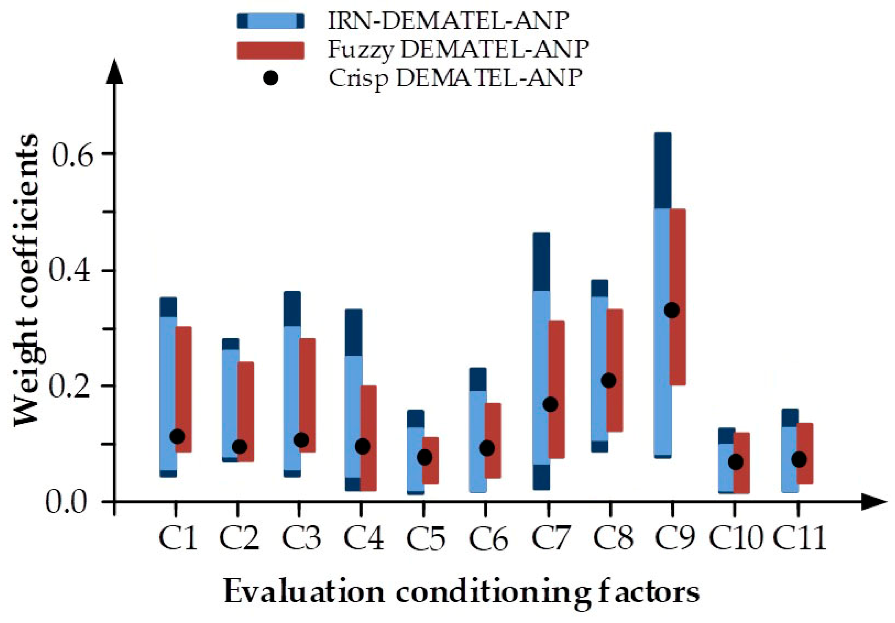
| Altitude (C1) | [(0.034,0.331),(0.040,0.337)] | 4 | 0.1002 |
| Slope (C2) | [(0.079,0.253),(0.071,0.272)] | 6 | 0.0910 |
| Curvature (C3) | [(0.034,0.303),(0.031,0.357)] | 5 | 0.0972 |
| TWI (C4) | [(0.015,0.237),(0.026,0.320)] | 7 | 0.0790 |
| STI (C5) | [(0.020,0.142),(0.053,0.186)] | 9 | 0.0538 |
| NDVI (C6) | [(0.023,0.224),(0.023,0.257)] | 8 | 0.0708 |
| Distance from rivers (C7) | [(0.022,0.368),(0.011,0.497)] | 3 | 0.1184 |
| Rainfall (C8) | [(0.091,0.378),(0.089,0.380)] | 2 | 0.1266 |
| Land cover/use (C9) | [(0.093,0.501),(0.091,0.656)] | 1 | 0.1776 |
| Lithology (C10) | [(0.012,0.107),(0.013,0.139)] | 11 | 0.0360 |
| Soil (C11) | [(0.023,0.153),(0.023,0.170)] | 10 | 0.0496 |
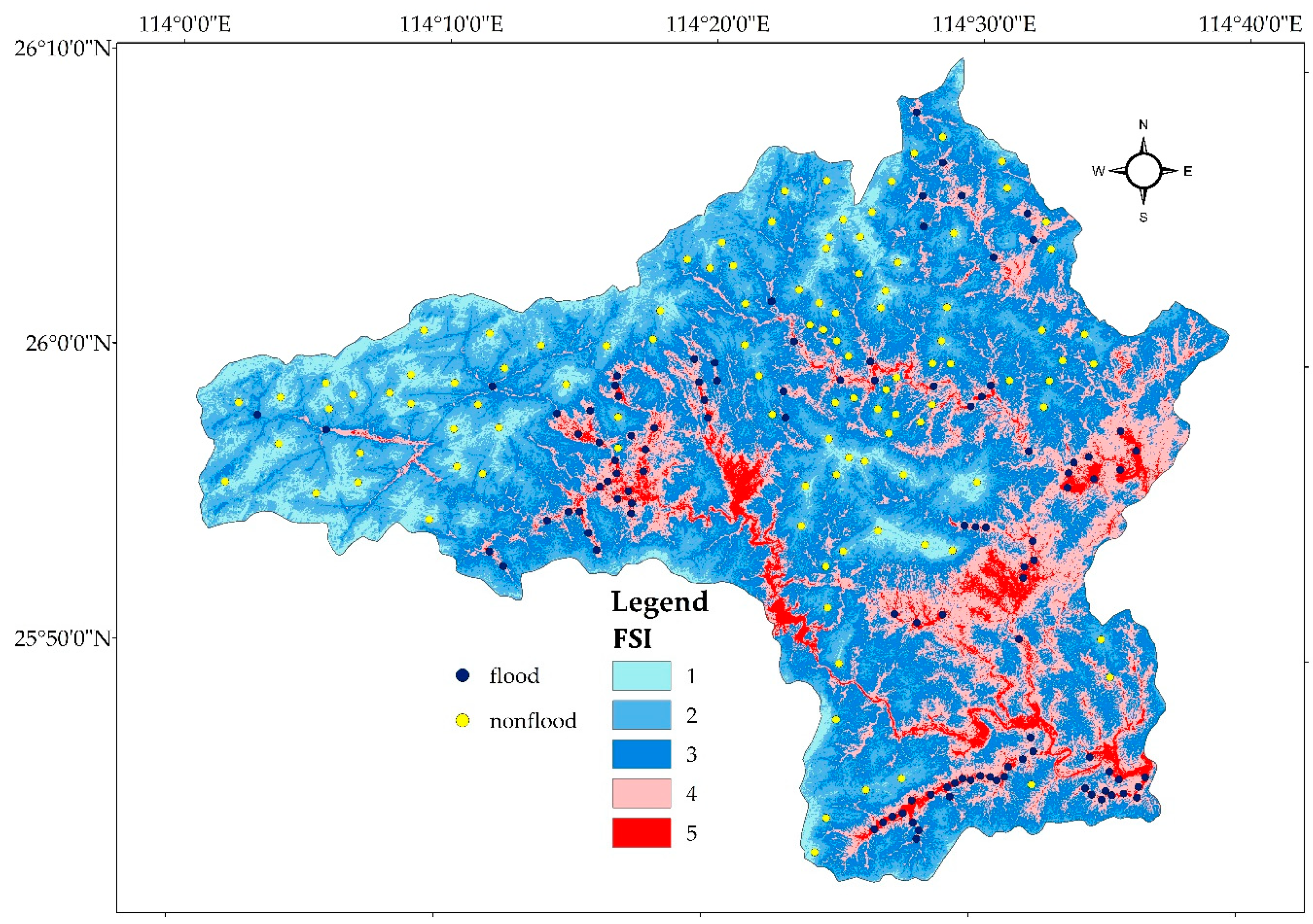
| FSI | Area | Number of Cells (30 × 30 m) | ||
|---|---|---|---|---|
| (km2) | % | |||
| FSI 1 | Very low | 118.4 | 7.7 | 131,544 |
| FSI 2 | Low | 434.8 | 28.2 | 483,080 |
| FSI 3 | Moderate | 588.4 | 38.1 | 653,747 |
| FSI 4 | High | 329.8 | 21.4 | 366,514 |
| FSI 5 | Very high | 71.6 | 4.6 | 79,534 |
© 2018 by the authors. Licensee MDPI, Basel, Switzerland. This article is an open access article distributed under the terms and conditions of the Creative Commons Attribution (CC BY) license (http://creativecommons.org/licenses/by/4.0/).
Share and Cite
Wang, Y.; Hong, H.; Chen, W.; Li, S.; Pamučar, D.; Gigović, L.; Drobnjak, S.; Tien Bui, D.; Duan, H. A Hybrid GIS Multi-Criteria Decision-Making Method for Flood Susceptibility Mapping at Shangyou, China. Remote Sens. 2019, 11, 62. https://doi.org/10.3390/rs11010062
Wang Y, Hong H, Chen W, Li S, Pamučar D, Gigović L, Drobnjak S, Tien Bui D, Duan H. A Hybrid GIS Multi-Criteria Decision-Making Method for Flood Susceptibility Mapping at Shangyou, China. Remote Sensing. 2019; 11(1):62. https://doi.org/10.3390/rs11010062
Chicago/Turabian StyleWang, Yi, Haoyuan Hong, Wei Chen, Shaojun Li, Dragan Pamučar, Ljubomir Gigović, Siniša Drobnjak, Dieu Tien Bui, and Hexiang Duan. 2019. "A Hybrid GIS Multi-Criteria Decision-Making Method for Flood Susceptibility Mapping at Shangyou, China" Remote Sensing 11, no. 1: 62. https://doi.org/10.3390/rs11010062
APA StyleWang, Y., Hong, H., Chen, W., Li, S., Pamučar, D., Gigović, L., Drobnjak, S., Tien Bui, D., & Duan, H. (2019). A Hybrid GIS Multi-Criteria Decision-Making Method for Flood Susceptibility Mapping at Shangyou, China. Remote Sensing, 11(1), 62. https://doi.org/10.3390/rs11010062