Using TSX/TDX Pursuit Monostatic SAR Stacks for PS-InSAR Analysis in Urban Areas

Abstract

Persistent Scatterer Interferometry (PS-InSAR) has become an indispensable tool for monitoring surface motion in urban environments. The interferometric configuration of PS-InSAR tends to mix topographic and deformation components in differential interferometric observations. When the upcoming constellation missions such as, e.g., TanDEM-L or TWIN-L provide new standard operating modes, bi-static stacks for deformation monitoring will be more commonly available in the near future. In this paper, we present an analysis of the applicability of such data sets for urban monitoring, using a stack of pursuit monostatic data obtained during the scientific testing phase of the TanDEM-X (TDX) mission. These stacks are characterized by extremely short temporal baselines between the TerraSAR-X (TSX) and TanDEM-X acquisitions at the same interval. We evaluate the advantages of this acquisition mode for urban deformation monitoring with several of the available acquisition pairs. Our proposed method exploits the special properties of this data using a modified processing chain based on the standard PS-InSAR deformation monitoring procedure. We test our approach with a TSX/TDX mono-static pursuit stack over Guangzhou, using both the proposed method and the standard deformation monitoring procedure, and compare the two results. The performance of topographic and deformation estimation is improved by using the proposed processing method, especially regarding high-rise buildings, given the quantitative statistic on temporal coherence, detectable numbers, as well as the PS point density of persistent scatters points, among which the persistent scatter numbers increased by 107.2% and the detectable height span increased by 78% over the standard processing results.

1. Introduction

Persistent Scatterer Interferometry (PS-InSAR) is a multi-temporal interferometric method that has been widely used for urban monitoring. Various cities use PS-InSAR as a standard monitoring tool for monitoring slow deformation, including ground [1,2,3,4], single buildings [5,6,7], and infrastructures [8,9]. The upcoming bi-static sensor missions promise even higher performance in global monitoring. In 2010, the TanDEM-X (TerraSAR-X Add-on for Digital Elevation Measurements) mission was launched. Together with TerraSAR-X (TSX), the constellation operates in a bistatic mode, with the primary goal of producing a highly accurate global digital elevation model (DEMs) of the Earth [10]. A secondary goal of the program is to demonstrate potential new applications of TanDEM-X (TDX) [11,12] and innovative new operating modes, including the bistatic, monostatic pursuit, and alternating bistatic modes, during the commissioning and scientific research phases of the mission [13,14]. Among those operation modes, the pursuit monostatic (PM) data is of interest for urban PS-InSAR applications that address slow motion, especially subsidence in urban areas.

In the PM mode, two satellites fly in the same orbit, one behind another, with an increased along-track baseline of 20 km, which is equal to a temporal baseline of 10 s. This enlarged distance allows both satellites to transmit and receive signals independently; thus, for each target scene, an independent image pair can be obtained within a time interval of 10 s. With this extremely short along-track temporal baseline between acquisitions within the PM mode, various applications on the datasets were conducted [15,16], and qualities were analyzed [17,18]. Few applications are found on urban areas [19], while most publications about PM data applications are focused on Moving Target Indication (MTI) [20,21], with examples drawn from sea surface derivation [22], and oil and ship detection [23]. Another example demonstrate the use of PM data for agricultural monitoring [24]. Many of the methods adopted in those publications are designed for change detection (CD), and are focused on minor changes of the targets occurring over short time intervals. Research on mono-static pursuit data for surface motion estimation, however, is limited; we assume that this is due to the limited availability of such stacks.

Upcoming Synthetic Aperture Radar (SAR) missions show similar constellations to TerraSAR-X and TanDEM-X; for example, TanDEM-L [25,26,27] or TWIN-L [28], will increase the availability of stacks of bi-static or PM image pairs considerably. In preparation for this, we use the technique of persistent scatter (PS) SAR interferometry for surface motion monitoring in urban areas. Although PM data allows for standard procedures without considering bi-static processing steps, processing PM data stacks with the standard PS-InSAR method does not make full use of the extremely short 10 s temporal baselines. Interferometric configuration in the standard PS-InSAR method tends to mix the topographic and deformation components in differential phase observations during estimations, especially in areas crowded with high-rise buildings; however, the interferometric phase generated by using only PM pairs is almost free from long-term deformation and atmospheric delay; hence, it is suitable for retrieving topographic residuals of urban areas, and the deformation estimation can thus be improved, especially regarding high-rise buildings, where spatially uncorrelated topographic residuals are commonly observed. Addressing this issue, we developed a new processing chain for PM data stacks, based on interferometry of PM pairs. The method will, in principle, be also applicable to bi-static stacks from the TanDEM-X mission, as well as future space-borne systems.

The paper is arranged as follows: in Section 2, the methodology of the processing is explained; in Section 3, the results of urban monitoring using pursuit monostatic spotlight acquisitions are demonstrated; in Section 4, the results are analyzed, and finally in Section 5, conclusions are drawn.

2. Materials and Methods

Principles of the standard PS-InSAR method are first stated in this section; after that, the proposed method will be presented based on the modification of the standard processing chain.

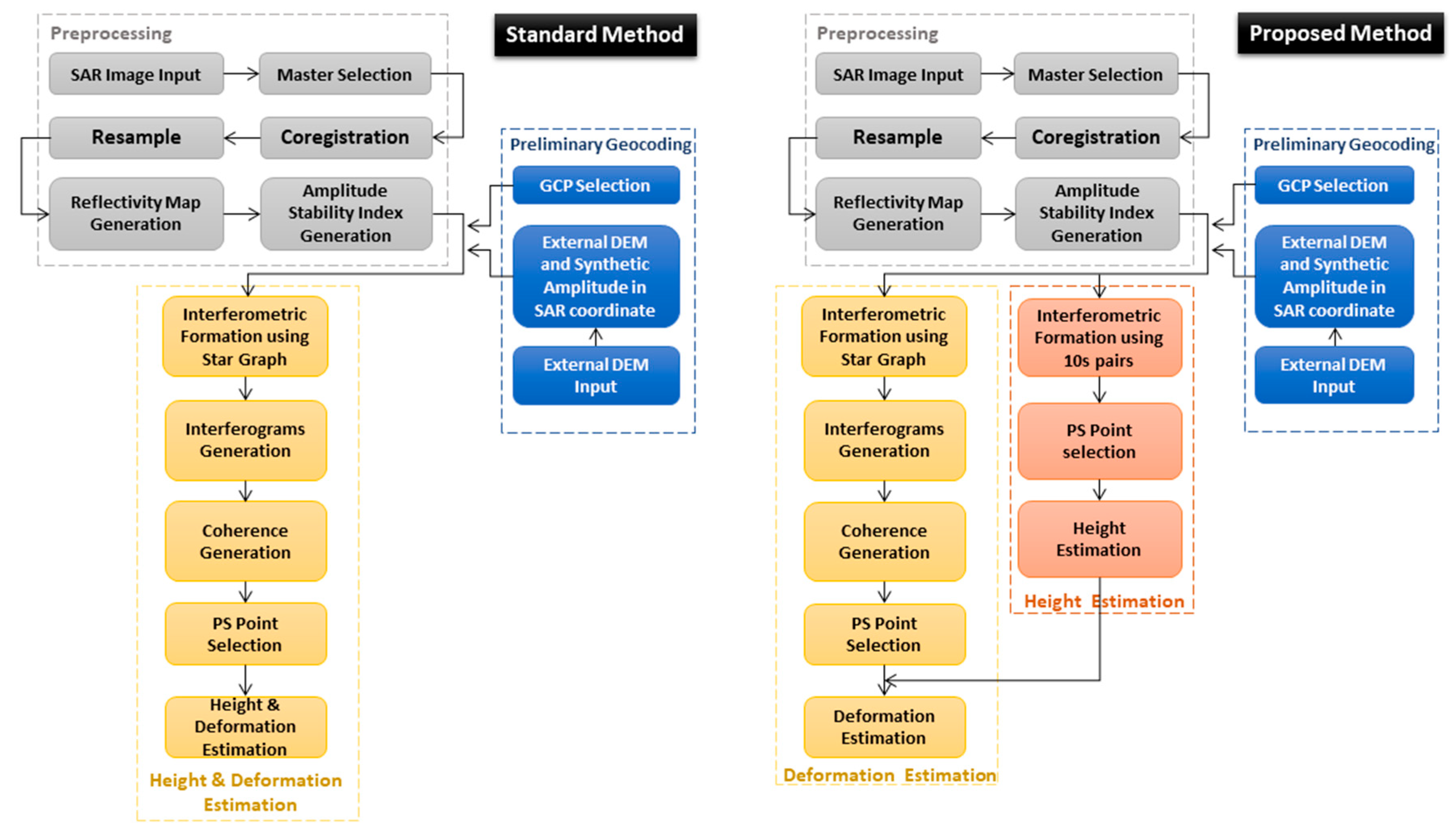
2.1. Standard PS-InSAR

The core of the standard PS-InSAR method is to conduct a time-series analysis of PS that can preserve stable backscattering over time. PS points can be selected based on several adoptable indexes, such as amplitude stability or temporal coherence. Selected PS points are connected to form a network; the deformation and topography differences for each arc are derived. The differential interferometric phase between the neighboring PS points is noted as:

$$\Delta {\varphi }_{diff}=\Delta {\varphi }_{defo}+\Delta {\varphi }_{\mathrm{topo}}+\Delta {\varphi }_{atmos}+\Delta {\varphi }_{noise}$$

(1)

$\Delta {\varphi }_{diff}$ express the differential interferometric phase, while ${\varphi }_{defo}$, $\Delta {\varphi }_{\mathrm{topo}}$, and $\Delta {\varphi }_{atmos}$ stand for the deformation, topographic, and atmospheric components of the differential interferometric phase. $\Delta {\varphi }_{noise}$ is the residual noise. The deformation component describes the deformation velocity difference between the neighboring PS points in the same arc. Both linear and non-linear deformation can be contained in this term; for example, urban subsidence [1] for linear deformation, and periodic thermal deformation [7] for non-linear deformation. The topographic component describes the residual topographic phase between neighboring PS points in the same arc. The atmospheric component describes phase change caused by phase delay during transmission, e.g. due to water vapor differences in the atmosphere. These three interferometric phase components, are main elements in the differential phase, together with non-linear deformation and noise, the equation can be extended as:

$$\Delta {\varphi }_{diff}=\frac{4\pi }{\lambda }T\Delta v+\frac{4\pi }{\lambda }\frac{B_{\perp }}{\rho \mathit{sin}\theta }\Delta h+\Delta {\varphi }_{atmos}+\frac{4\pi }{\lambda }\Delta D_{non-linear}+\Delta {\varphi }_{noise}$$

(2)

In this equation, λ is the wavelength, T is the temporal baseline, ρ is the slant range, and θ is the incident angle. $\Delta {\varphi }_{diff}$ is the differential observation; the linear deformation velocity Δv and the residual topographic phase Δh are the unknowns. If the actual differential phase is bigger than 2π, phase ambiguities also need to be considered in the resolution process, which are also unknowns. The atmospheric component $\Delta {\varphi }_{atmos}$ can be mitigated by spatial filtering, or optionally supported by introducing an external water vapor mapping product. It can also be estimated within standard PS-InSAR, which will be mentioned in the later paragraphs. The atmospheric component $\Delta {\varphi }_{atmos}$, non-linear deformation component ΔD_non-linear, and noise term $\Delta {\varphi }_{noise}$ are considered as residual phase $\epsilon$, as we can see in:

$$\epsilon =\Delta {\varphi }_{atmos}+\frac{4\pi }{\lambda }\Delta D_{non-linear}+\Delta {\varphi }_{noise}$$

(3)

Nevertheless, distances between PS candidates (PSC) within the PSC network can be controlled within certain limits, and the area of triangles in this network can be restricted to be small enough either, hence the residual phase ε of differential observations can normally be considered to be no bigger than $\pi$; therefore, phase ambiguities can be assumed to be zero. If the number of images in one interferograms stack is M, differential observations generated between the neighboring PS points x and y can be formulated as:

$$\Delta {\varphi }_{x-y,ifg}^k=\left[{\alpha }^k,{\beta }^k\right]·\left[\begin{array}{c}\Delta {\nu }_{x-y}\\ \Delta h_{x-y}\end{array}\right]+\epsilon \left(k=1,2,\dots ,M\right)$$

(4)

where $\Delta {\varphi }_{x-y,ifg}^k$ is the differential interferometric phase generated between x and y, k is the index of interferograms, α^k and β^k are the coefficients of mean velocity Δv_x-y and the residual topographic phase Δh_x-y; Δv_x-y and Δh_x-y are unknowns, and they have to be determined under maximized temporal coherence γ.

To solve for the mean velocity Δv_x-y and the residual topographic phase Δh_x-y in Equation (4), periodogram spectral analysis [29] is applied in the standard PS-InSAR technique. The method can transform the residual phase into a frequency domain in space {Δh, Δv}, and search for the location of single PS points that could maximize the temporal coherence γ. This method is based on the original wrapped interferograms, and the performance of this method depends on the temporal and spatial distribution of baselines; with an increased number and a more even distribution of the temporal baseline, the performance could be improved.

The atmospheric component is also estimated, together with mean velocity Δv_x-y and the residual topographic phase Δh_x-y. After estimation of the topographic error and deformation for each point along the network based on a previously selected sparse PSC network, their topography and deformation can be derived, starting from a selected reference point. The remaining phase residuals caused by atmospheric effects and are subsequently used to estimate the atmospheric phase screen (APS) of each interferogram. The atmospheric components in differential phases can be extracted through low-pass filtering in the spatial domain, and high-pass filtering in the temporal domain [30]. On this basis, the APS of each interferogram can be obtained by interpolation, using various methods, for instance, kriging. After removing the APS, the deformation and topographic error for every PSC in the stack are estimated relative to the previously selected reference point.

After determination of Δh and Δv, the topography and deformation can be derived for each PS point. Topographic components for each PS point can be resolved within an indirect adjustment model, and can be abbreviated as:

$$\Delta h_{M\times 1}=C_{M\times N}\times h_{N\times 1}$$

(5)

where M is the number of PS connection arcs, N is the number of selected PS points, Δh is the residual topographic observation, h is the unknown PS topography, and C is the coefficient matrix describing the relationship between residual topographic phase Δh between neighboring PS points and the topography h for each PS point, which is also what we referred as PS height. In response to least-square principle, the solution for this function is:

$$h_{N\times 1}={\left(C_{N\times M}^T{P}_{M\times M}{C}_{M\times N}\right)}^{-1}{C}_{N\times M}^T{P}_{M\times M}\Delta h_{M\times 1}$$

(6)

In Equation (6), P is weight matrix. On the other hand, deformation pattern may not necessarily be linear. As we consider the whole scene, the topographic phase between neighboring PS points may also lead to phase wrapping in the spatial domain. In this context, the topographic component is considered as an error source and deformation is extracted based on the resumed interferometric phase after removal of the topographic components. Phase unwrapping is applied to the interferograms, and various algorithms can be chosen, for instance, Branchcut [31], SNAPU [32], etc. The unwrapped interferometric phase is noted as:

$${\varphi }_{x,uw}^k={\varphi }_{x,defo}^k+{\hat{\varphi }}_{x,topo}^k+{\hat{\varphi }}_{x,atmos}^k+{\hat{\varphi }}_{x,noise}^k$$

(7)

where ${\varphi }_{x,uw}^k$ expresses the unwrapped phase, ${\varphi }_{x,defo}^k$ expresses the deformation component, and ${\hat{\varphi }}_{x,topo}^k$, ${\hat{\varphi }}_{x,atmos}^k\mathrm{and}{\hat{\varphi }}_{x,noise}^k$ express the topographic, atmospheric components as well as the noise term of the unwrapped phase, respectively. After removal of the topographic component and the estimated atmospheric component from the interferometric phase, the residual phase can be considered as deformation signal. Converting the deformation phase ${\hat{\varphi }}_{x,topo}^k$ into the slant-range deformation distance d, $d={\varphi }_{defo}\cdot \lambda /4\pi$ together with the temporal baseline t, according to least-square principle, the deformation velocity within each time interval can be resolved as:

$$v={\left(t^{\prime }Pt\right)}^{-1}Pd$$

(8)

In this equation, v is the expected deformation velocity, P is the weight matrix, d is the slant range deformation distance, and t is the temporal baseline.

In practical image processing, the processing chain is implemented using SARProZ (Daniele Perissin, RASER Limited, Hong Kong) [33], in which the standard PS-InSAR can be divided into four parts that are listed below:

• Preliminary processing: image import; master selection; co-registration; resampling; reflectivity map generation; amplitude stability index generation;
• Preliminary geocoding: ground control point (GCP) selection; external DEM input; projection of external DEM and synthetic amplitude in SAR coordinates; Mask for PSCs;
• APS estimation: interferometric formation using star graph; select a subset of PSCs according to a certain threshold; triangulation of sparse PSC network and generation of differential phase; deformation and topographic estimation based on given search space; selection of reference point; inversion of initial APS;
• Sparse estimation: interferometric formation using star graph; selection of all PSCs based on a certain threshold; Input of initial APS, differential phase and reference points; deformation and topographic estimations based on the given search space for the PSCs.

However, applying the standard PS-InSAR approach to a PM data stack does not provide the best possible solution. As mentioned in the first section, there are two kinds of temporal baselines in PM data stacks: normal temporal baselines between repeat-pass intervals of the same satellite, which is 11 days for our case, and the extremely short 10 s temporal baselines between the acquisition times of TSX and TDX satellites at the same repeat-pass interval. These short temporal baselines are also a feature of this PM data. The interferometric phase generated with 10 s pairs are less likely to contain deformation components and also are less affected by atmospheric delay, consequently making these interferometric phases contain mainly the topographic phase component. As the deformation and residual topographic phase are estimated together in standard PS-InSAR, an external estimated height with the 10 s pairs could provide more accurate residual topography values for deformation estimation, thus allowing for a better performance of urban target monitoring.

2.2. A PS-InSAR Solution for Mono-Static Pursuit Datasets

To explore the full potential of these interferometric phases generated with 10 s pairs, and to refine the performance of deformation estimation, we propose a new processing chain that separates topographic error estimation from velocity estimation. The purpose is to use the 10 s pairs for topographic error estimation so that influences of un-modeled deformation and APS can be largely avoided. We assume that the retrieved topographic error would be better estimated with this modification; when measuring deformation and calculating APS, we use these precise topographic error estimations; in this way, the precision of the overall processing will be increased. This new processing chain is especially advantageous for areas with high-rise buildings, where large spatially uncorrelated topography errors occur.

Our proposed processing chain is similar with the standard PS-InSAR processing chain mentioned in Section 2.1. The preliminary processing steps and geocoding steps are the same. We read the SAR image data stack, select a common master image, and co-register all slave images to this master and resample. The reflectivity map and amplitude stability index are generated for each pixel based on this co-registered data stack. External Digital Elevation Models (DEM) are used, in order to simulate the spatial correlated topographic component. After this conventional preprocessing, APS and sparse estimations are implemented by using a modification of the original PS-InSAR processing chain.

In the proposed processing chain, both APS and sparse estimation are processed in two rounds; the first round aims for the residual topographic estimation, and the second round for the deformation. In round one, the interferometric formation of the PM data are connected only between the 10 s pairs, as shown in the real example used in our experiment listed below.

According to Figure 1, the interferometric phases are generated between SAR acquisitions derived from TSX and TDX satellites that fly within a temporal baseline of 10 s. Topographic errors, instead of deformation velocities, are estimated in this formation, since the generated interferometric phases are free from atmospheric delay. Furthermore, as we are working in urban areas, the temporal decorrelation for man-made targets is negligible, making this an ideal configuration for height estimation. Nevertheless, given that interferometric phases are less affected by atmospheric delay or by long-term deformation, regular spatial correlated error such as orbital error may still have some impact on the differential phase generated from these interferometric phases.

Once estimation for the residual topographic error is completed, we reprocess the stack in round two, connecting the interferograms in time. In our experiments, we used a standard single master approach, and as shown in Figure 2, all of the slave images are connected to a common master image in a star graph. However, other approaches, e.g., SBAS-like, are also possible.

Deformation estimation is conducted in this round, considering the residual topographic phase derived previously in the first round; after removing this component, the deformation phase is unwrapped and the mean velocity of each PS point is resolved according to Equation (9). In summary, the processing chain of the proposed method is listed below:

• Preliminary processing: image import; master selection; co-registration; resampling; reflectivity map generation; amplitude stability index generation;
• Preliminary geocoding: GCP selection; external DEM input; projection of external DEM and synthetic amplitude in SAR coordinates; Mask for PSCs;
• First APS estimation: interferometric formation using only 10 s PM pairs; selection of a subset of PSCs according to a certain threshold; triangulation of sparse PSC network and generation of the differential phase; topographic estimation only based on a given search space; selection of the reference point; inversion of the initial APS;
• First sparse estimation: interferometric formation using only 10 s PM pairs; selection of all PSCs based on a certain threshold; input of initial APS, differential phase, and reference point; topographic estimation only based on the given search space for PSCs;
• Second APS estimation: interferometric formation using a star graph; selection of a subset of PSCs according to a certain threshold; triangulation of sparse PSC networks and generation of a differential phase; deformation estimation based on residual phase components derived in the first round within a given search space; selection of the reference point; inversion of the initial APS;
• Second Sparse estimation: interferometric formation using star graph; selection of all PSCs based on a certain threshold; Input of initial APS, differential phase and reference point; deformation estimation based on the residual phase component derived in first round within a given search space for PSCs;

The specific flow charts of both the standard and our proposed processing chains are briefly shown in Figure 3.

3. Experiment Results

Both processing chains mentioned in Figure 3 are tested with a pursuit-monostatic dataset acquired over our study area in Guangzhou. The results are presented separately in this section. Specific information on our study area and dataset information are also demonstrated below.

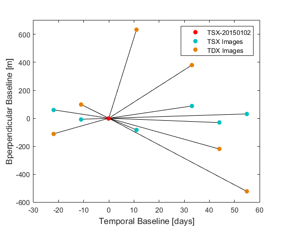
3.1. Study Area and Dataset Information

Guangzhou is one of the most developed cities in China, where rapid economic development brings many new buildings in recent years. Our study area is displayed in the yellow square shown in Figure 4, which covers the central area of the Zhujiang New Town Central Business District (CBD).

This is an extremely dense urban area with dozens of skyscrapers. The landmark buildings in this area include the CTF Finance Centre (539.2 m), known as Canton East Tower, and Guangzhou International Finance Centre (440.75 m), known as West Tower. These two are the tallest two buildings in this area. Other tall buildings such as Universal Plaza (318 m), Guangcheng International mansion (360 m), Pearl River Tower (309 m), Leatop Plaza (303 m), and Fuli Ying Kai Plaza (296.4 m), are among the top 10 highest buildings in Guangzhou. They are marked with pentagons in Figure 4. Also, the Guangzhou Opera House, the Guangdong Museum, and the Haixinsha Asian Games Theme Park are located in the south of Zhujiang New Town. These are located along the two sides of the so-called Automated People Mover System (APM), together with the skyscrapers, as we can see in the blue north–south traffic line in that passes though the central area of Zhujiang New Town CBD. Therefore, this area is marked as the central part of our test site, as shown in the orange region in Figure 4.

Apart from the central area, there are also tall buildings around the central area. The general distribution of the buildings with different heights is very different in our study area, though according to the approximate average heights of buildings, the study area could be divided into several sub-regions, if one street block is counted as a single unit. Here, we sorted the sub-regional urban surface into three categories. The first one is the central CBD marked in orange; with many skyscrapers, the average height of this area is very high. The second one is the newly built residential areas, where many tall buildings with height limits are distributed. These residual areas include urban communities, shopping districts, and public service buildings, such as schools, hospitals, and tax bureaus. Due to the height limit of 100 m according to the definition of “high-rise buildings” given by the General code for civil building design (GB50352-2005), these residual buildings, marked in the pink regions, are typically not higher than 100 m. The rest of the test site are old residual areas in Guangzhou with building heights not exceeding 50 m; residual apartments with eight floors about 24 m are the most common.

Based on the three categories, we select two small regions in our test site, i.e., test region A and B, marked with dashed boxes in Figure 4 for simple analysis in the experiment. These two regions cover the first two typical types of urban areas, as mentioned above, and demonstrate the different features in height distribution. Two subsets, the central area and central east area in test region A, are further selected for their high density of tall buildings, named subregions 1 and 2, shown as purple and orange areas, respectively, in Figure 4.

The Pursuit Monostatic data stack used in the experiment contains 14 ascending staring spotlight (ST) images, i.e., seven TSX/TDX mono-static pursuit pairs during 11 December 2014 to 26 February 2015. Other specific parameters about the dataset are listed in

Table 1. Dataset information of pursuit monostatic data in Guangzhou.

Operation Mode	Pursuit Mono-Static
Image Mode	Staring Spotlight (ST)
Look Angle	43.4°
Polarization	VV
Direction	Ascending
Resolution	0.24 m (azimuth)
	0.80 m (ground range)
Azimuth Extent	3 km
Range Extent	5.5 km
External Information	Acquisition Time	Temperature (°C)
	20141211	14.5
	20141222	9.1
	20150102	11.6
	20150113	11.2
	20150204	12.4
	20150215	16.7
	20150226	22.0

.

3.2. Experimental Results

Experimental results obtained in processing these pursuit monostatic data using both standard and proposed processing chains are displayed in the following paragraphs.

3.2.1. Processing Results from the Standard Method

The Pursuit Monostatic dataset in the Guangzhou test site is first processed with the standard processing method. Preprocessing and preliminary geocoding are accomplished according to the steps listed in Section 2.2. Interferometric formations of SAR images are configured in a star graph, using a single master as shown in Figure 2.

After generating interferograms and coherence, initial PS candidates are selected based on the amplitude stability, index with a threshold of 0.2. Although 0.3 is usually sufficient for urban monitoring, we set this threshold to be slightly lower, because the image resolution of the staring spotlight data is high enough to ensure abundant reliable PS points in the results. In this result, we select 740,105 PSC according to our threshold; the temporal coherence of these PSC points after processing is shown in Figure 5.

In this result, the PSCs generally demonstrate good temporal coherence, as we can see in Figure 5A, where most of PSC coherence values are distributed in the numerical interval [0.6, 1], especially PSCs from the ground and from lower parts of building façades. Their temporal coherence is mostly distributed in [0.8, 1], as the red points shown in Figure 5. Nevertheless, we can still find some relative unstable PSCs, shown in yellow in Figure 5A. These yellow points are mainly distributed along the façades of high-rise buildings, especially in the central area and its surrounding regions marked in Figure 4, as we can see in the enlarged coherence map in test regions A and B, as shown in Figure 5B,C. The triangle icons in Figure 5A,B represent skyscrapers with heights above or around 300 m. By comparing the coherence maps of the test regions A and B, we can find some unstable PSCs that have clear shapes of buildings edges, but there is a shift between the actual locations and the derived locations from standard processing results. These unstable PSCs are referred to “shifted PSCs” in our experience, and their shifts in location can be found around skyscrapers in Figure 5B. In Figure 5C, where most of the buildings are residential buildings that have a height limit of 100 m, much less shifted PSCs are found.

After selecting the initial PSCs according to the amplitude stability index, the estimation of deformation and topographic residuals are implemented, together within a total resolving of the differential phases, based on the least-square principles, according to Equation (4). Deformation and topographic residuals of PSCs are accomplished by setting pre-defined search spaces between −100 to 100 mm/year for linear deformation, and −300 m to 300 m for topographic residuals, since the vast majority of PSCs are expected to fall into this interval. 343,965 PS points are extracted, with temporal coherences of larger than 0.97 and their estimated topographic residuals, or residual height maps, are shown in Figure 6.

The resulted PS point residual heights range from −288.8 m to 168.5 m, with a mean value of 27.3 m. As we can see from Figure 7, a majority of the PS points detected in this result are points with low heights, since ground points, i.e., green points, are dominant in the map. High PS points can also be found in high-rise building areas, as we can see in the test regions A and B; however, the detectable height is limited, and only found in the lower part or the bottom of the buildings; this is clearer in the 3D demonstration of the PS-InSAR result in test region A, as shown in Figure 7.

The deformation map is shown in Figure 8. A total of 343,963 PS points were selected with a temporal coherence bigger than 0.85 and amplitude stability index smaller than 0.2. As we can see from Figure 8, most ground points are stable, while in the southeastern part of our test site, a subsidence pool can be found.

Clear structured PS point clusters can be found and they show significant negative motion, i.e., motion away from the sensor in the line-of-sight direction. The shape of these point clusters indicate that they are part of high-rise buildings, but they show a shift between the location of these point clusters and normal PS points of the same structure; as mentioned in previous paragraphs, these clusters are referred as “shifted PS” and their presence is assumed to be caused by geocoding error, with an inaccurate estimation of topographic residuals. A clearer view of this deformation result is shown below, in which a 3D deformation map of a small area in test region A is displayed.

We can see more clearly that in Figure 9, thermal expansions are also visible on high-rise buildings where velocity is accumulated along with height. An estimation with seasonal deformation could be applied to remove the thermal deformation, as mentioned in Crosetto et al. [7]; however, the mono-static pursuit data has only seven pairs, covering a time span of just three months, which is not enough to model the temperature-related deformation correctly.

3.2.2. Processing Results from Our Proposed Method

After processing the pursuit monostatic data using the standard processing chain, we continue to process these data using the proposed processing chain. Preprocessing and preliminary geocoding are also accomplished according to the steps listed in Section 2.2. Topographic residuals and deformation estimation steps are accomplished in separated processing rounds. Topographic residuals are accomplished in the first round, with interferometric formation set in accordance with Figure 1.

In this test, PSCs are selected with the same amplitude stability index used in the standard processing steps; the topographic component of PSCs is retrieved in a least square process, assuming that only topographic residuals are left in the interferometric phase. Meanwhile, the temporal coherence of the PSCs is also generated, as shown in Figure 10.

Figure 10 shows that an overwhelming majority of PS points demonstrate very high temporal coherence distributed in the numerical interval [0.9, 1], even in areas with many high-rise buildings in test regions A and B, as displayed in the enlarged coherence map in Figure 10B,C. Also, we do not find shifted PSCs in this result. The point number and general stability of the PSCs are largely improved in our proposed processing results.

Residual height map generated in the proposed processing chain is displayed in Figure 11 and visualized in 3D in Figure 12, with a pre-defined search span for height estimation set between −300 m to 300 m.

A total of 712,760 PS points were extracted with the same coherence threshold of 0.97 being used for displaying the results from standard processing. As we can see in Figure 11, the PS heights in the high-rise building areas are fully detected. The detectable height limit is largely improved in this result, ranging from −294.9 m to 300 m, with an average height of 38.1 m. For skyscrapers, the height estimation is also largely improved, as the detectable PS points on the buildings are increased from the ground or the bottom to the full façades, as we can see in the 3D image of test region A below.

These PS heights are restored and used in the following deformation estimation. The interferometric formation is set according to Figure 2, where the identical star graph is adopted. Deformation estimation is thus accomplished based on pre-derived topographic residuals. Consequently, the linear deformation results are shown in Figure 13, where 465,564 PS points with a temporal coherence larger than 0.85 are selected, with an amplitude stability index smaller than 0.2.

Deformation patterns in Figure 13 shows similar results compared to Figure 8, with a subsidence pool detected in southeastern area of our test site. This subsidence signal can be more clearly observed in Figure 13, as we can see that the shifted PS clusters in Figure 9 disappear in our proposed processing results. As we assume, this is due to the large reduction of topographic errors during the height estimation using only PM pairs. This improvement of topographic residual estimations further improves the deformation estimation accuracy. Although we still cannot estimate the temperature-related motion with only seven TSX and TDX pairs, with increased detectable height limits in our proposed processing method, the thermal deformation is also improved. For the same single building, the detected deformation velocity grows larger than that in the standard processing results, especially for skyscrapers in the central area, as we see in 3D demonstration of PS deformation in Figure 14.

4. Discussion

To evaluate the performance of these two processing chains, the results of the two processing chains are compared and analyzed in this section, on the basis of quantitative statistics. PS point properties are discussed in three aspects, including temporal coherence, and topographic and deformation estimation.

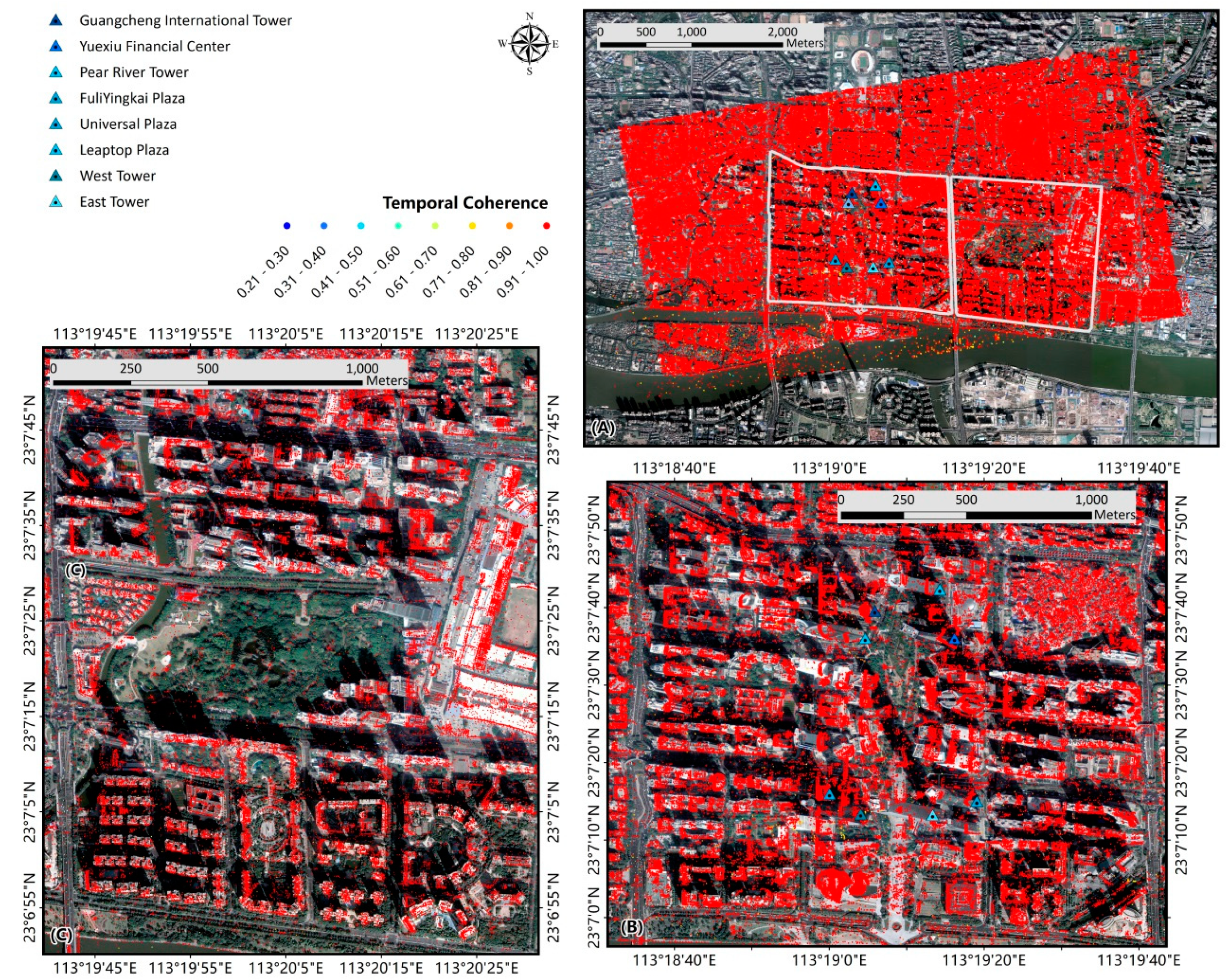
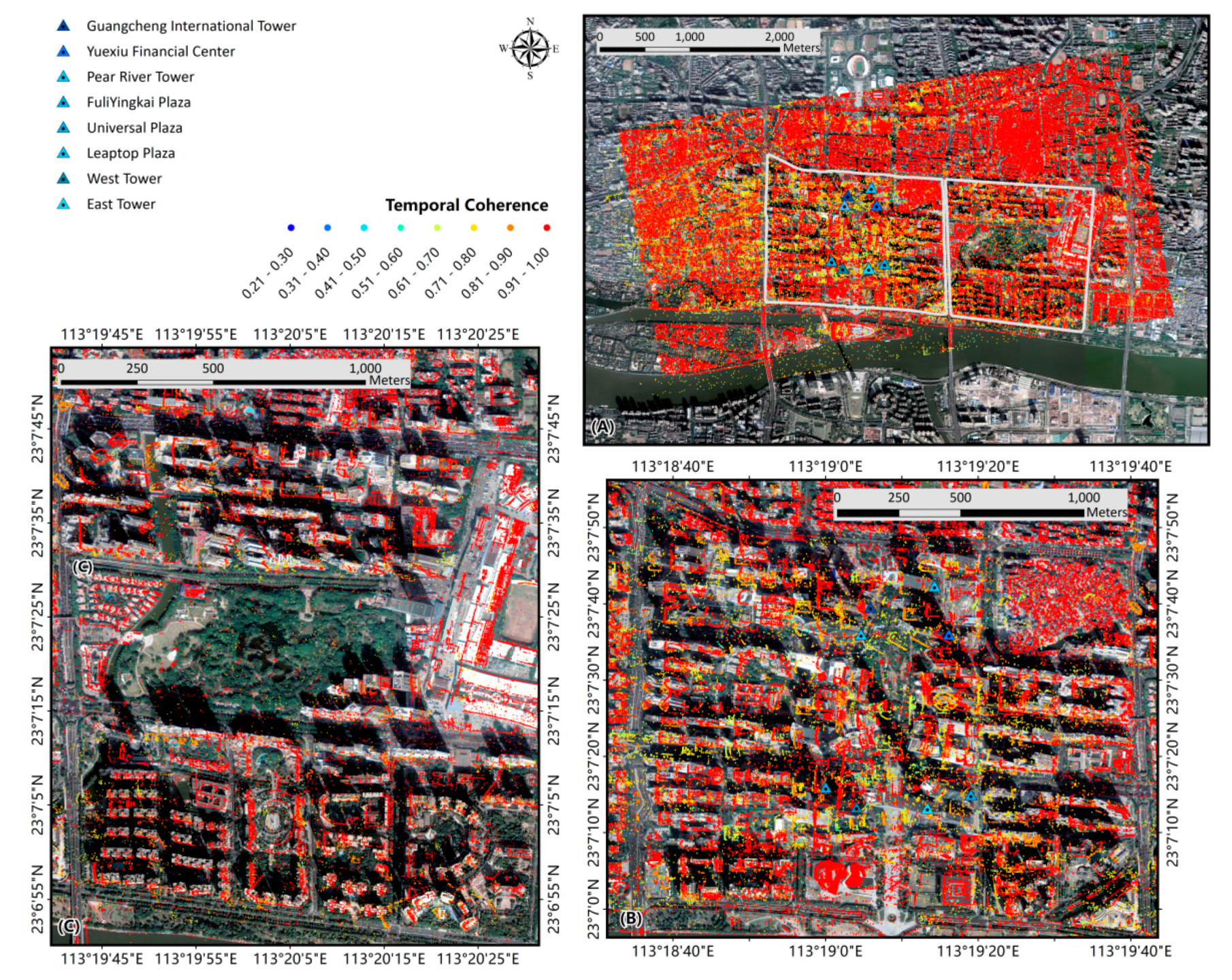
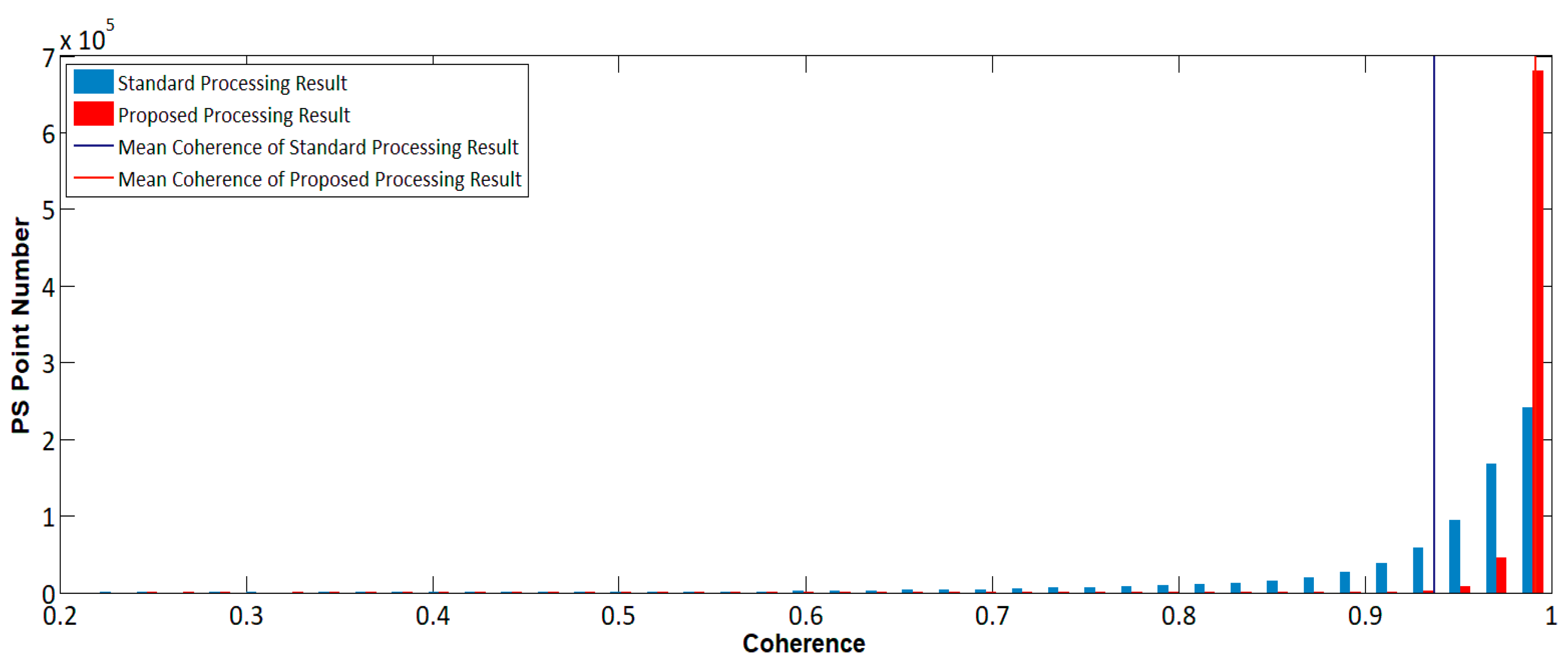
4.1. Temporal Coherence

The temporal coherence of PSCs selected using the same threshold in both standard and proposed processing chains are analyzed according to the histogram shown in Figure 15. A histogram of PS points for temporal coherence in both standard and proposed processing results.

The histogram was generated, taking 0.02 as bin distance. The blue and red bars express the PS numbers in each bin; Blue and red vertical lines express the mean height value of the total PS heights, for standard and proposed processing results respectively. As we can infer from Figure 15, the persistent scatterers from the proposed method demonstrate a steeper distribution in the histogram, with quicker increase in PS numbers in high coherence intervals, compared to PSs derived from the standard processing result. The mean temporal coherence of the proposed processing result, 0.99, is also bigger than the mean temporal coherence, 0.94, of the standard processing result, which indicates a generally higher stability of PSs in the proposed processing results, as well as less disturbance in the phase observations. Topography estimation using these PSs is more likely to obtain accurate results.

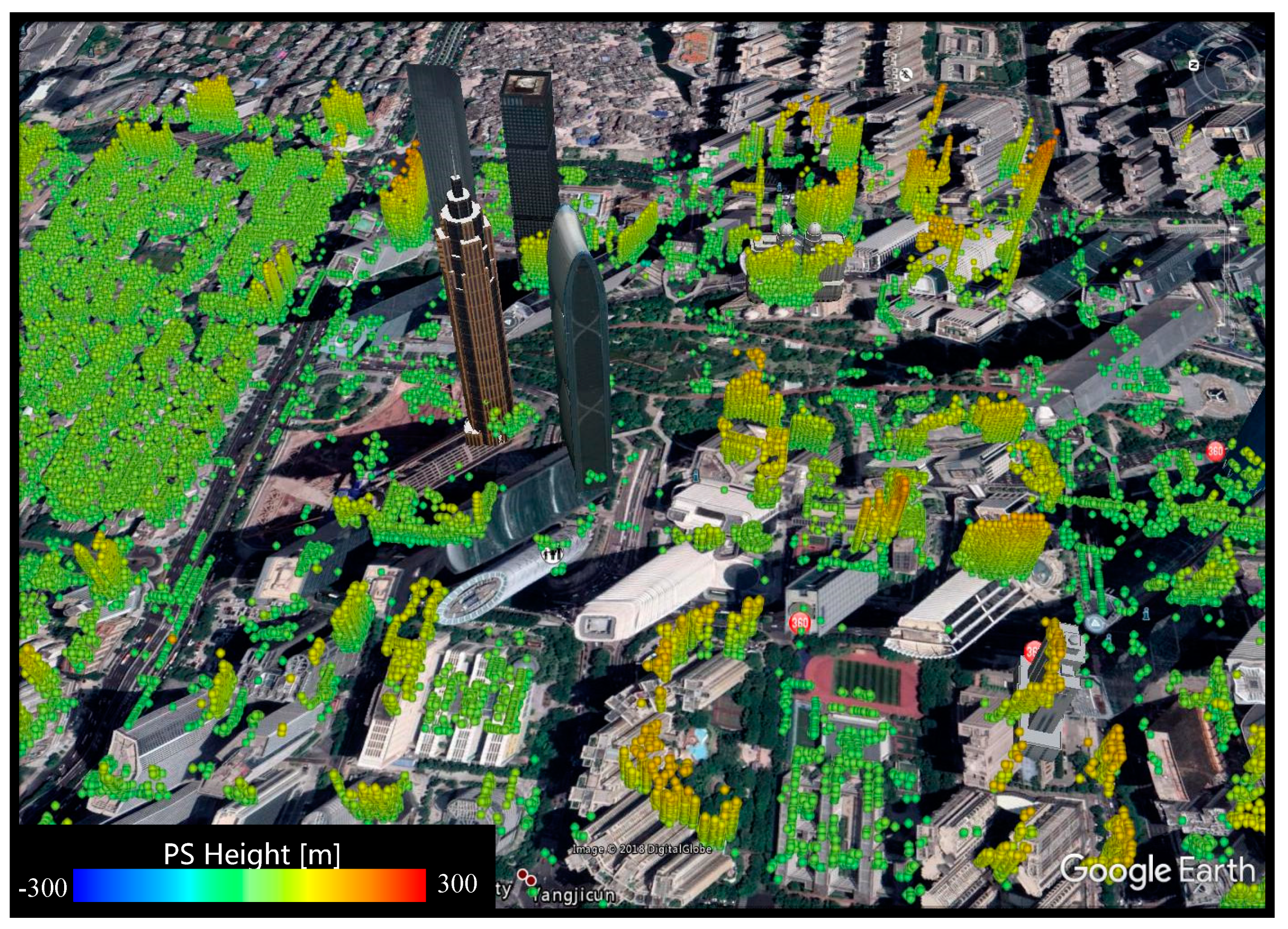
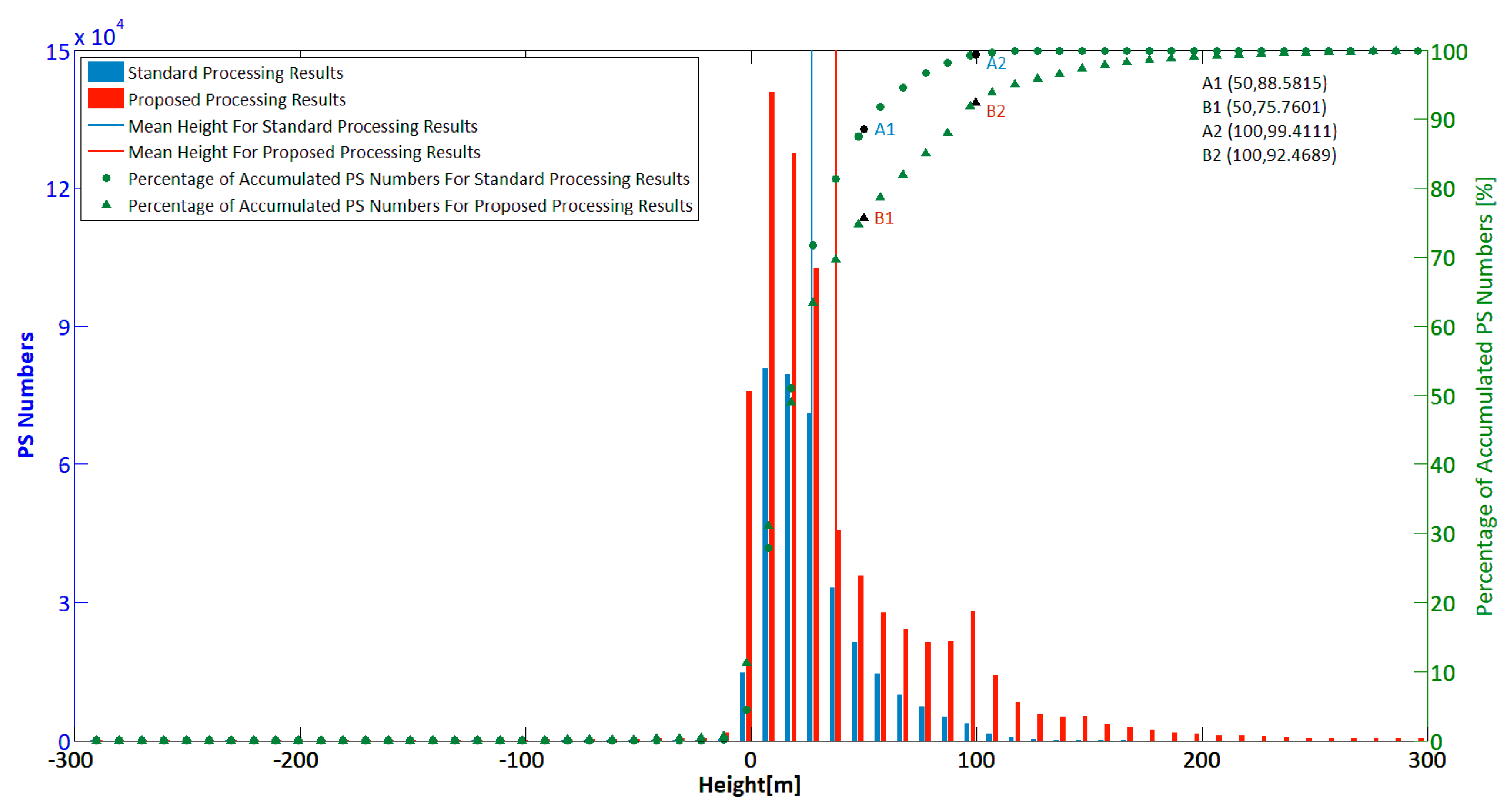
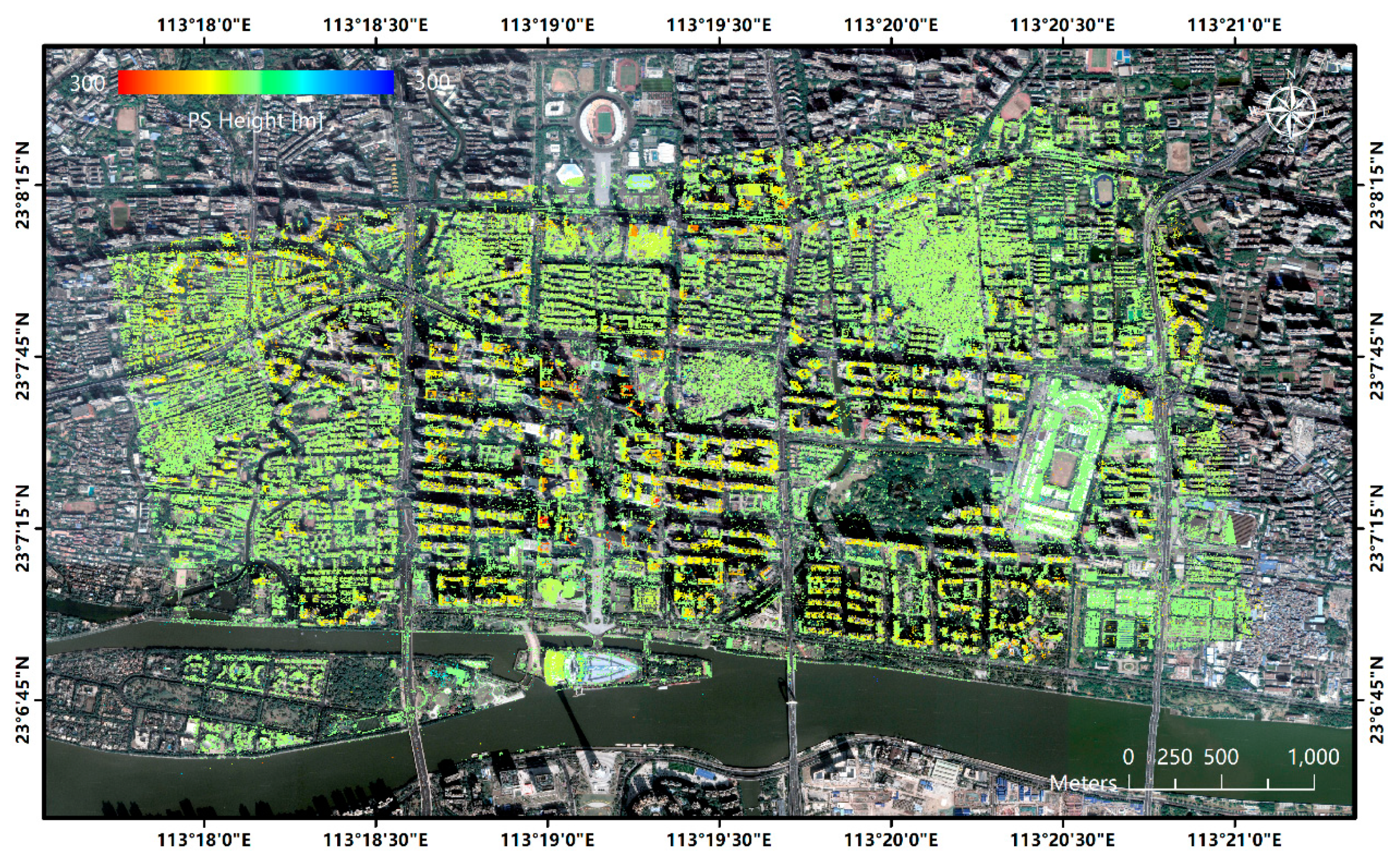
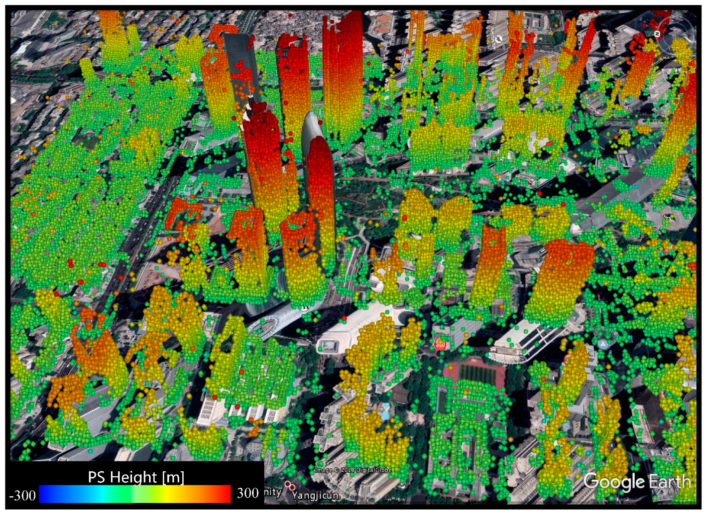
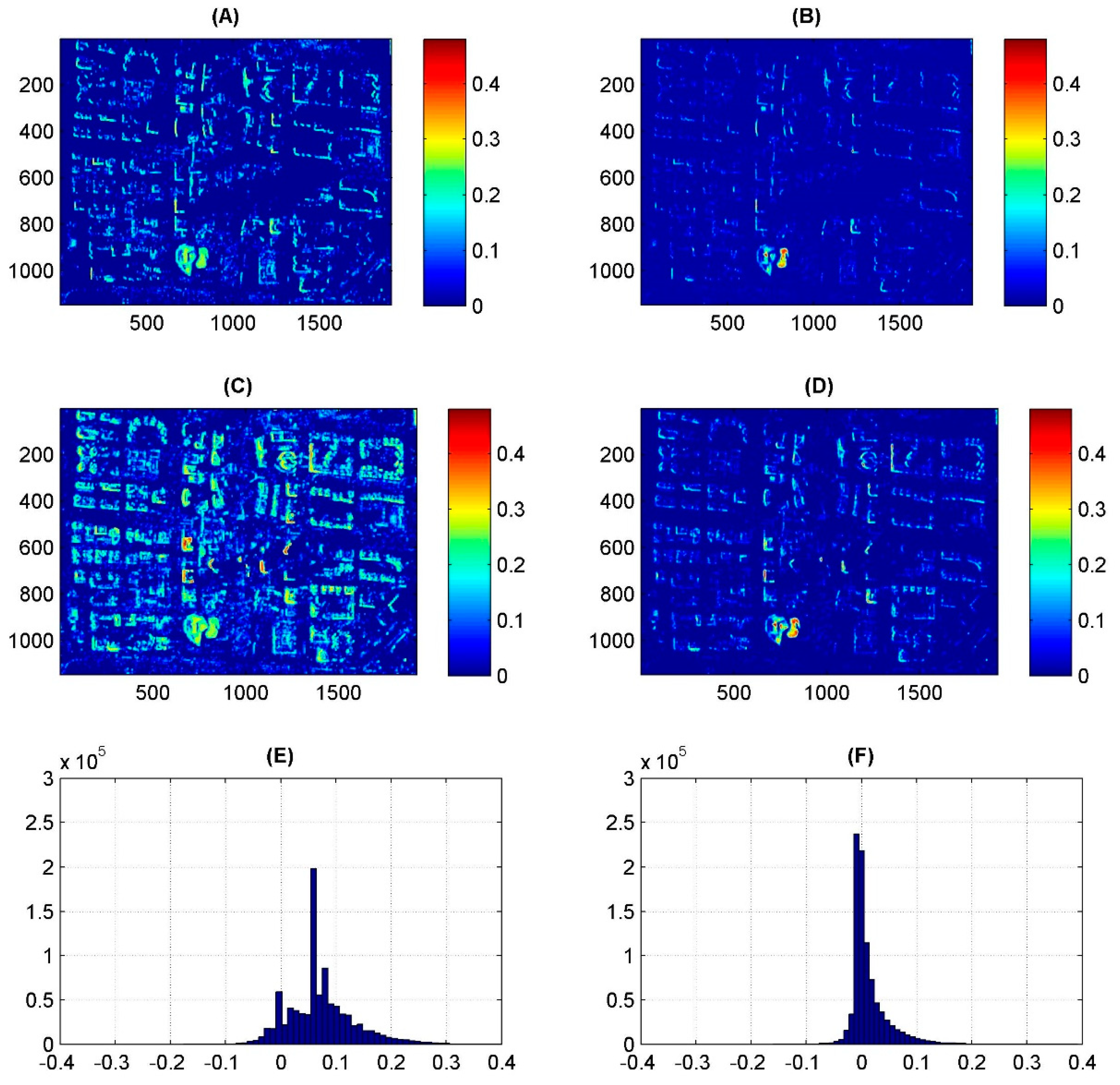
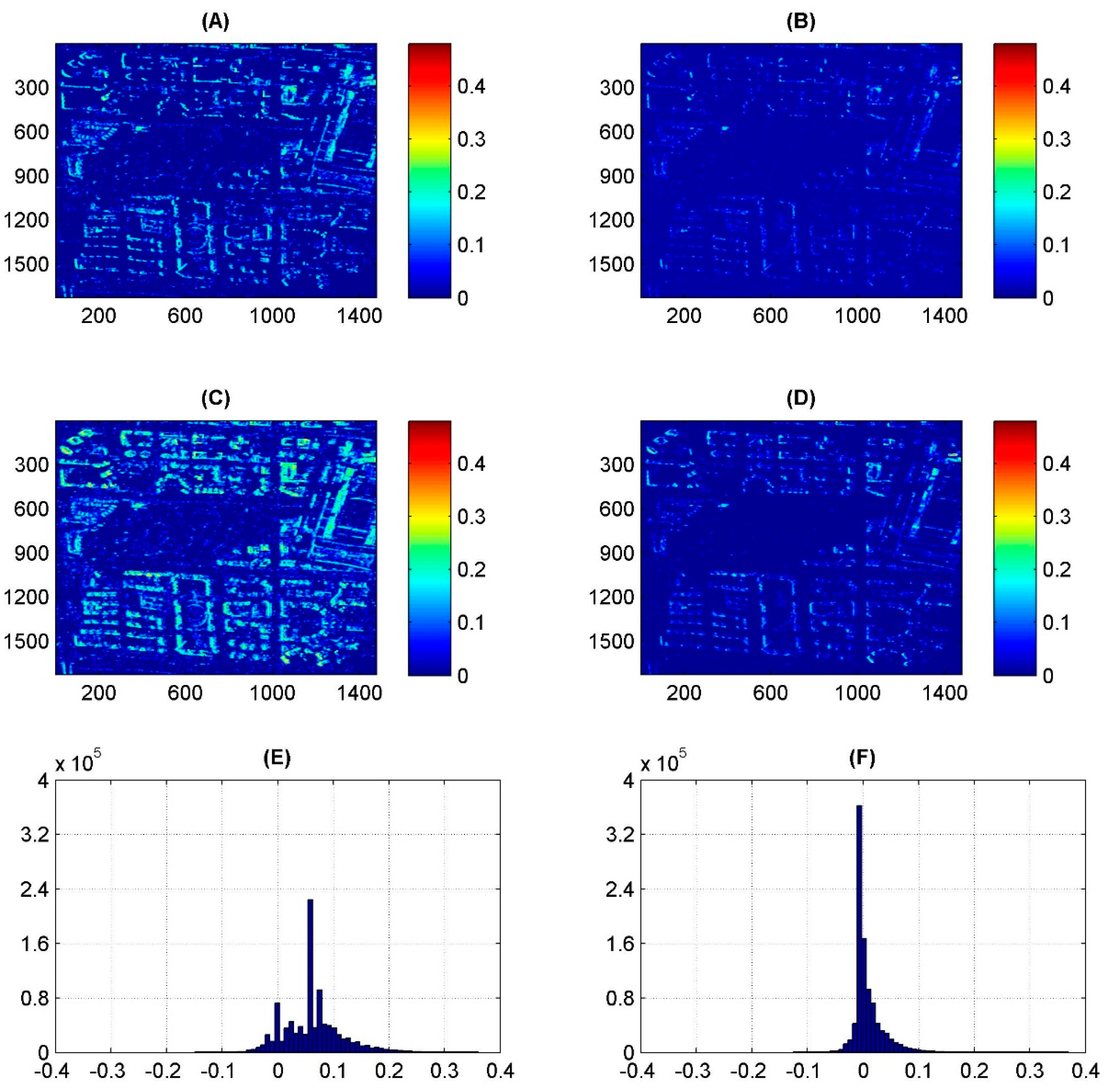
4.2. Topography Estimation

Topography estimation results are also quantitatively analyzed, mainly focusing on PS point numbers and density.

4.2.1. PS Point Numbers

Histogram of PS point heights for both standard and proposed processing results are presented with a distance bin of 5 m, as shown in Figure 16.

The blue and red bars represent PS point numbers in each bin of PS height for the standard and proposed processing results, respectively. The blue and red vertical lines represent the mean height value of the total PS points in stand and proposed processing results, respectively. The green dotted lines express the accumulated PS numbers for the standard processing results as a percentage; meanwhile, the green triangle lines express the accumulated PS numbers for the proposed processing results as a percentage. As we can infer from Figure 16, for PS points selected with the same temporal coherence threshold, more PS points are detected in each height bin in the proposed processing results, than in the standard processing results, with an overall rate of increase of 107.2%, and 663% in the 100 m bin. Also, the detected PS height span is increased from the standard processing results to the proposed processing results, from 168.5 m to 300 m, increased by 78%. The majority of PS heights are distributed in interval from 0 to 50 m.

The percentage curves of accumulated PS numbers, marked in green circle and triangle icons in Figure 16, also reveals that more than 88% of the PS points are distributed in height intervals between 0 to 50 m in standard processing results, as marked with A1, which are assumed to be ground or low building points. About 99.4% of the total PS points have height values below 100 m, marked in A2; and only around 0.6% percent of the PS points are detected over targets with heights bigger than 100 m. On the other hand, for proposed processing results, 76% percent of the detected heights are below 50 m, as marked with B1, and 92.4% of the PS points are below 100 m, marked with B2; the other 7.6% of the detected PS heights are between 100 m and 300 m. There is also a local peak of PS numbers with a height value around 100 m; this is in accordance with the emergence of high-rise buildings, which are built under the height limit of 100 m. These increased number of PS points with heights around 100 m are assumed to be building roofs. This comparison shows the limited detection ability of standard processing method on high-rise buildings, comparing to proposed processing results, especially for high-rise buildings.

4.2.2. Persistent Scatterer Density

Apart from the general increase of the PS points, the PS point density is further estimated based on the statistics of the variance and mean value of a PS point. This variance is defined as the square deviation of the estimated height values within a patch centered on each PS point with extension of 10 m; the mean value of a PS point is defined as the mean height value of all PS points within the patch. The statistical results of variance and mean value, as well as the differences between these two, are calculated and normalized. The sub region 1 and 2 are selected as our test regions as we can see in Figure 4. The Statistical results of these values are listed below.

Figure 17 and Figure 18 demonstrate variance and mean values, as well as the difference histogram of these two indexes. The variance of the PS points in the proposed processing results increases in our test region, compared to the standard processing results, as most of the variance difference is positive in the histograms; the detectable locations are also expanding in the proposed processing method. As we know, façade PS points are vertically distributed on buildings, so that if the variance gets bigger, it could be either caused by an increased point density within a certain height limit, or an increased detected height limit. In this context, the mean value of the test region is also presented. The mean value of the test region is slightly increased; as we infer from the mean value difference histogram from both Figure 17 and Figure 18, the difference value is distributed around 0, but it has a larger positive span. As we can see in the distribution map, PS points with an increased mean value are mostly derived from building façades. Hence, we can infer from these statistics of the variance and mean value that the point density on the building façades is increasing. Besides, in the statistical result of the central area of Zhujiang CBD, increased variances are detected. For the skyscrapers in the central area, the variance and mean value map increases, which is a hint towards the increase of the point density and the detected heights, which is also in accordance with the 3D visualization of these areas in Figure 7 and Figure 12.

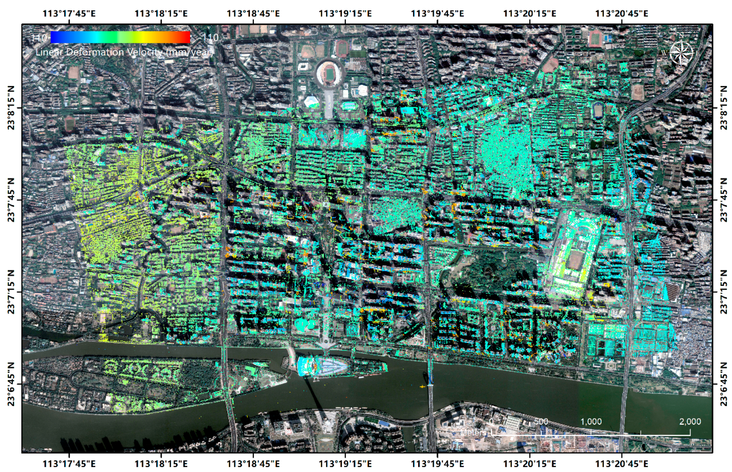
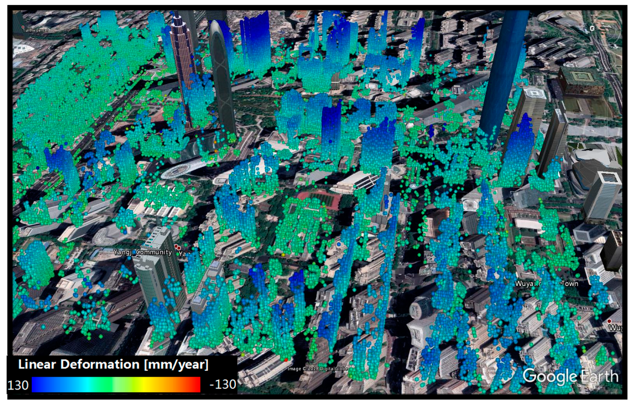
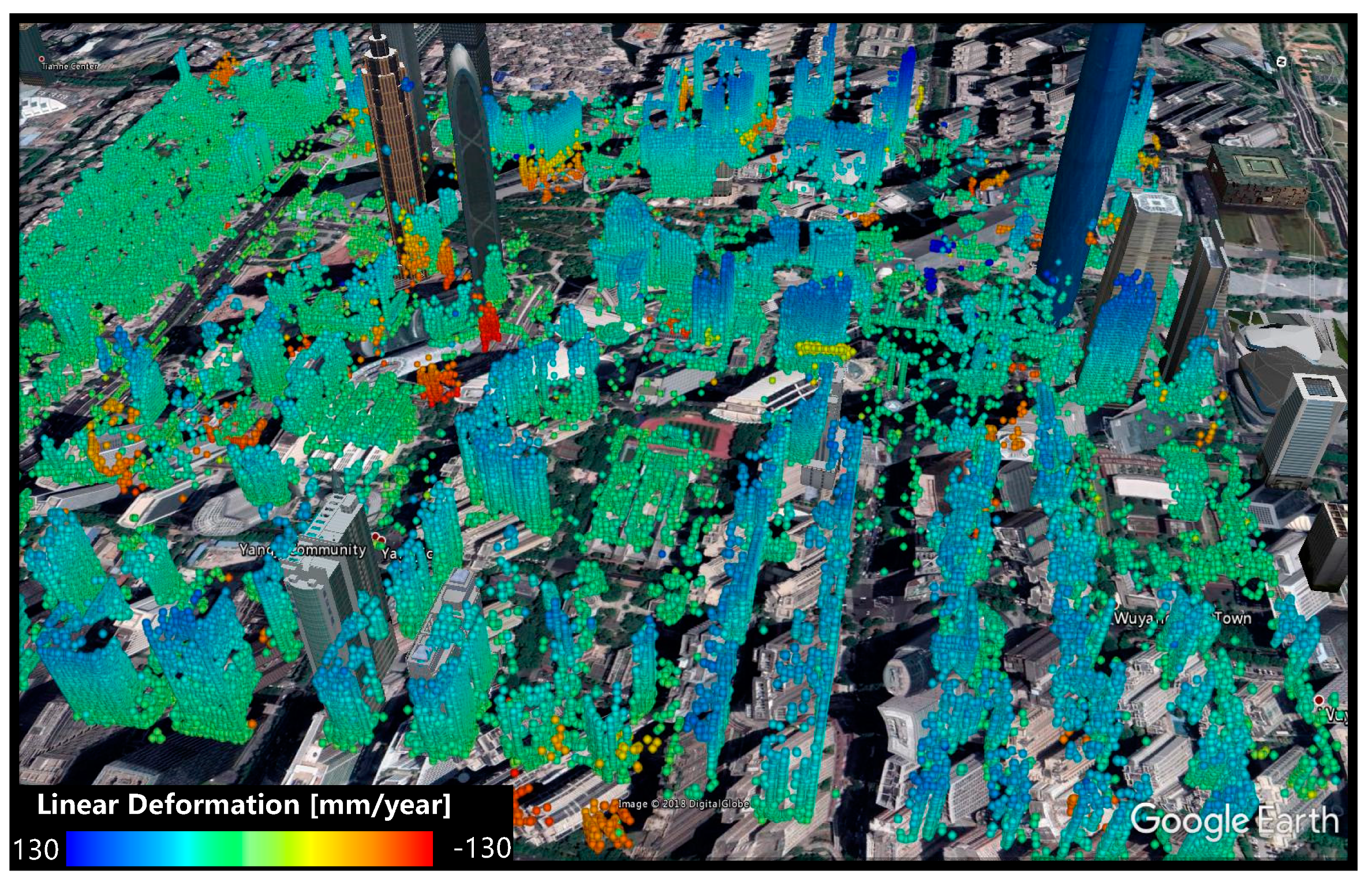
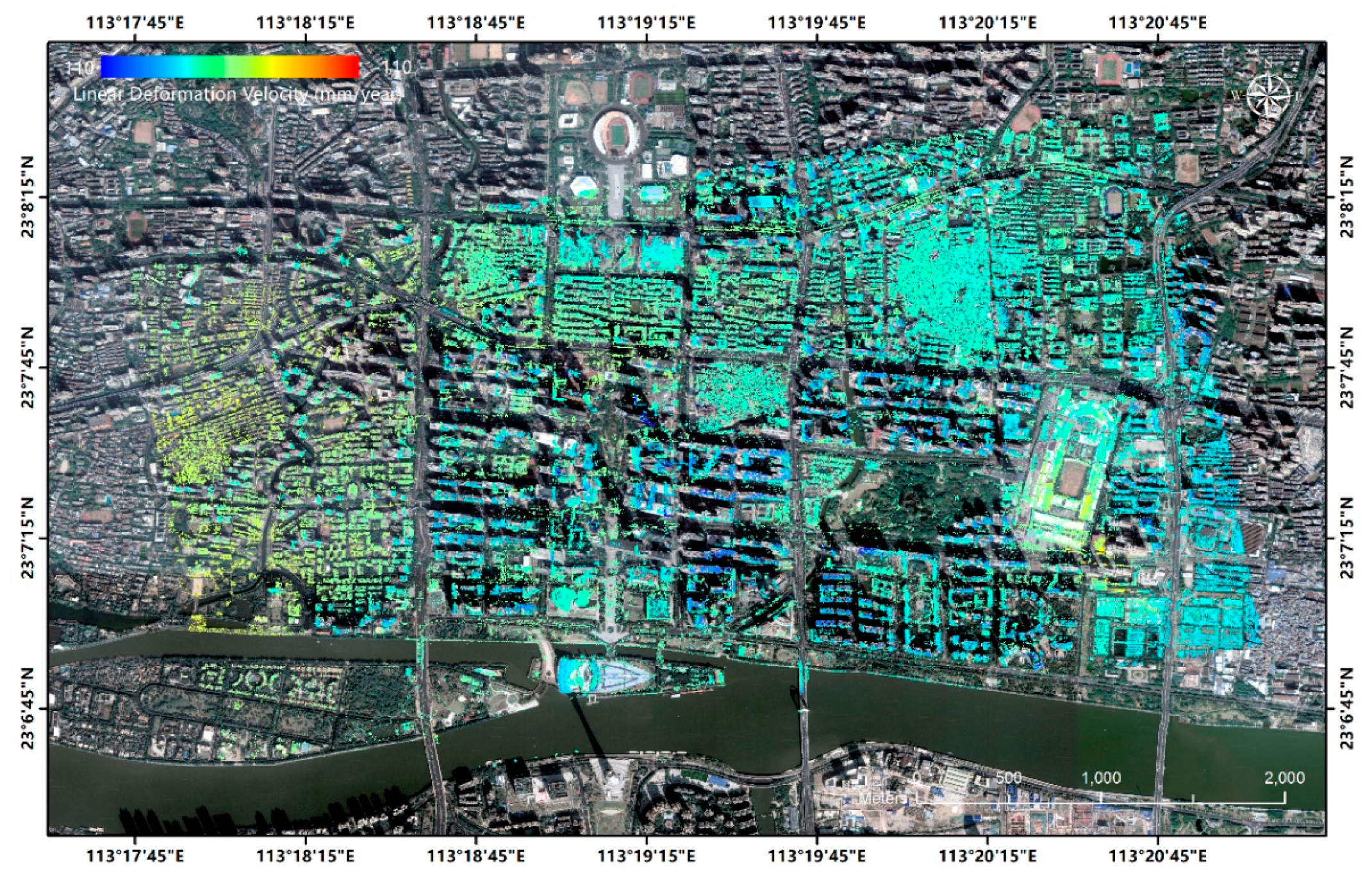
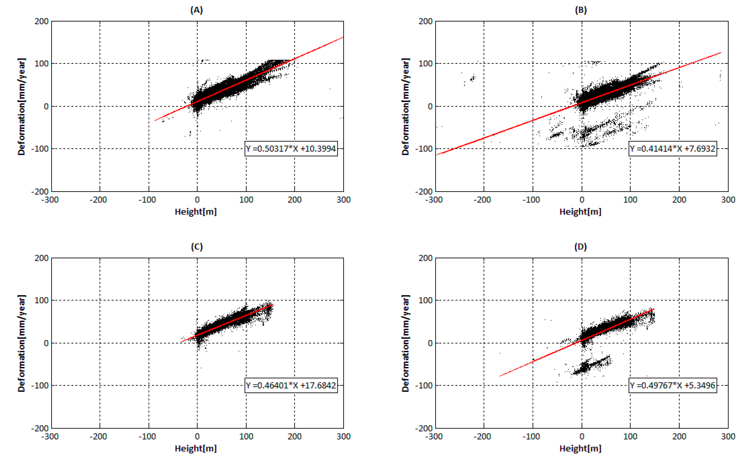
4.3. Deformation Estimation

Comparisons of surface motion estimated from the standard method and our proposed methods are also addressed, as we can see in Figure 8 and Figure 13. Similarities can be found in these two results: first, for PS near the ground, both results show good performance, as we can see in the northeastern part of our results. The traffic lines can be clearly seen in the northeastern corner of our test site. Second, the same subsidence patterns can be detected in the southeastern part of our study area. A linear ramp could be detected in the deformation maps, which is assumed to be caused by orbital error, such orbital effects can occur due to the limited number of the images, the special nature of the data acquired, and the baseline distribution during the science phase of the project.

For deformation results, the main improvement from our proposed processing method lies in the removal of the shifts and refinements of thermal deformation in the high-rise building area. Since the thermal deformation in the high-rise buildings accumulated from the bottom to the top of buildings, a linear relationship exists between the thermal deformation and the PS height. This linear relation is also due to the short overall time-span of the data acquisition. For data stacks covering a longer time period, we would rather expect a sinusoidal behavior. However, in our example, a linear regression analysis is accomplished, in order to evaluate this refinement. The results are demonstrated below.

As we can see in Figure 19, there is a clear linear relationship in the regression result in sub-region 1 and 2, with deformation and height in the central area. It can be inferred that the deformation changes faster along with height in the proposed processing, as we can see in the specific slope in Figure 19A,C, compared to Figure 19B,D. The reason for this increase in the linear slope is the removal of shifts, as well as an increased number of PS points detected on high façades, which increases the detectable span of the temperature-related deformation, thus enlarging the proportion of larger deformations in the results. The absolute value of this deformation could be corrected if we had more image pairs covering a longer period. Furthermore, we can see that we can estimate points at much higher positions correctly.

However, when processing the deformation, influences from the atmosphere are unavoidable. For ground subsidence monitoring, the main deformation trends can be found with the standard PS-InSAR processing, as well as our proposed method. We can see differences and reduced noise in our approach. For monitoring high-rise buildings, and especially for skyscrapers, shifts during estimation are refined, and the linear relationship between the deformation and PS height are better restored. However, the number of images, and especially of image pairs, is very limited in both stacks, which leads to imperfect results, as the number of images is too low to successfully estimate temperature-related deformation. Nevertheless, we demonstrate improvements when using our proposed approach, and its practical significance for mono-static pursuit and bi-static data stack processing.

5. Conclusions

Urban monitoring is an important issue in China. With upcoming SAR missions, e.g., TanDEM-L and Twin-L, the application of innovative SAR products in urban monitoring has to be explored. Pursuit monostatic data is tested in this paper as an example, but the results can also be used for bi-static stacks. A direct application of this data to standard PS-InSAR shows only a restricted ability for urban monitoring and does not make full use of the extremely short temporal baselines, which are the characteristic of the pursuit monostatic pairs. In this context, a new processing method is proposed on basis of the standard PS-InSAR method in this paper. Both proposed and standard PS-InSAR processing methods are tested with pursuit monostatic staring spotlight data in Guangzhou. The detectable PS numbers and height span using the proposed processing method are largely increased by 107.2% and 78%, respectively. For surface motion estimations near the ground surface, both methods achieve similar performances. For deformation estimation in high-rise buildings, shifts that occurred in the standard processing results are fixed with the proposed processing. Based on the experimental results mentioned above, we conclude that the proposed processing method demonstrates better ability in urban monitoring, and it is a more suitable choice for monostatic pursuit and bi-static data.

References

1. Ferretti, A.; Prati, C.; Rocca, F. Nonlinear subsidence rate estimation using permanent scatterers in differential SAR interferometry. IEEE Trans. Geosci. Remote Sens. 2000, 38, 2202–2212. [Google Scholar] [CrossRef]
2. Lanari, R.; Zeni, G.; Manunta, M.; Guarino, S.; Berardino, P.; Sansosti, E. An integrated SARGIS approach for investigating urban deformation phenomena: A case study of the city of Naples, Italy. Int. J. Remote Sens. 2004, 25, 2855–2862. [Google Scholar] [CrossRef]
3. Colesanti, C.; Mouelic, S.L.; Bennani, M.; Raucoules, D.; Carnec, C.; Ferretti, A. Detection of mining related ground instabilities using the Permanent Scatterers technique—A case study in the east of France. Int. J. Remote Sens. 2005, 26, 201–207. [Google Scholar] [CrossRef]
4. Vallone, P.; Giammarinaro, M.S.; Crosetto, M.; Agudo, M.; Biescas, E. Ground motion phenomena in Caltanissetta (Italy) investigated by InSAR and geological data integration. Eng. Geol. 2008, 98, 144–155. [Google Scholar] [CrossRef]
5. Gernhardt, S.; Adam, N.; Eineder, M.; Bamler, R. Potential of very high resolution SAR for persistent scatterer interferometry in urban areas. Ann. GIS 2010, 16, 103–111. [Google Scholar] [CrossRef]
6. Gernhardt, S.; Bamler, R. Deformation monitoring of single buildings using meter-resolution SAR data in PSI. ISPRS J. Photogramm. Remote Sens. 2012, 73, 68–79. [Google Scholar] [CrossRef]
7. Crosetto, M.; Monserrat, O.; Cuevas-González, M.; Devanthéry, N.; Luzi, G.; Crippa, B. Measuring thermal expansion using X-band persistent scatterer interferometry. ISPRS J. Photogramm. Remote Sens. 2015, 100, 84–91. [Google Scholar] [CrossRef]
8. Qin, X.; Zhang, L.; Yang, M.; Luo, H.; Liao, M.; Ding, X. Mapping surface deformation and thermal dilation of arch bridges by structure-driven multi-temporal DInSAR analysis. Remote Sens. Environ. 2018, 216, 71–90. [Google Scholar] [CrossRef]
9. Qin, X.; Zhang, L.; Ding, X.; Liao, M.; Yang, M. Mapping and Characterizing Thermal Dilation of Civil Infrastructures with Multi-Temporal X-Band Synthetic Aperture Radar Interferometry. Remote Sens. 2018, 10, 941. [Google Scholar] [CrossRef]
10. Schulze, D.; Zink, M.; Krieger, G.; Böer, J.; Moreira, A. TANDEM-X mission concept and status. In Proceedings of the FRINGE, Frascati, Italy, 30 November–4 December 2009. [Google Scholar]
11. Fritz, T.; Rossi, C.; Yague-Martinez, N.; Rodriguez-Gonzalez, F.; Lachaise, M.; Breit, H. Interferometric processing of TanDEM-X data. In Proceedings of the IEEE International Geoscience and Remote Sensing Symposium (IGARSS), Vancouver, BC, Canada, 24–29 July 2011; pp. 2428–2431. [Google Scholar]
12. Fritz, T.; Breit, H.; Rossi, C.; Balss, U.; Lachaise, M.; Duque, S. Interferometric processing and products of the TanDEM-X mission. In Proceedings of the IEEE International Geoscience and Remote Sensing Symposium (IGARSS), Munich, Germany, 22–27 July 2012; pp. 1904–1907. [Google Scholar]
13. Hajnsek, I.; Krieger, G.; Papathanassiou, K.; Baumgartner, S.; Rodriguez-Cassola, M.; Prats, P. TanDEM-X: First scientific experiments during the commissioning phase. In Proceedings of the 2010 8th European Conference on Synthetic Aperture Radar (EUSAR), Aachen, Germany, 7–10 June 2010; pp. 1–3. [Google Scholar]
14. Bachmann, M.; Hofmann, H. Challenges of the TanDEM-X commissioning phase. In Proceedings of the 2010 8th European Conference on Synthetic Aperture Radar (EUSAR), Aachen, Germany, 7–10 June 2010; pp. 1–3. [Google Scholar]
15. Prats, P.; Scheiber, R.; Mittermayer, J.; Wollstadt, S.; Baumgartner, S.V.; López-Dekker, P.; Schulze, D.; Steinbrecher, U.; Rodríguez-Cassolà, M.; Reigber, A.; et al. TanDEM-X experiments in pursuit monostatic configuration. In Proceedings of the 2012 9th European Conference on Synthetic Aperture Radar (EUSAR), Nürnberg, Germany, 23–26 April 2012; pp. 159–162. [Google Scholar]
16. Lumsdon, P.; Schlund, M.; von Poncet, F.; Janoth, J.; Weihing, D.; Petrat, L. An encounter with pursuit monostatic applications of TanDEM-X mission. In Proceedings of the IEEE International Geoscience and Remote Sensing Symposium (IGARSS), Milan, Italy, 26–31 July 2015; pp. 3187–3190. [Google Scholar]
17. Bello, J.L.B.; Martone, M.; Gonzalez, C.; Kraus, T.; Bräutigam, B. First interferometric performance analysis of full polarimetric TanDEM-X acquisitions in the pursuit monostatic phase. In Proceedings of the IEEE International Geoscience and Remote Sensing Symposium (IGARSS), Milan, Italy, 26–31 July 2015; pp. 1242–1245. [Google Scholar]
18. Bueso-Bello, J.L.; Martone, M.; Prats-Iraola, P.; González-Chamorro, C.; Kraus, T.; Reimann, J.; Jäger, M.; Bräutigam, B.; Rizzoli, P.; Zink, M. Performance Analysis of TanDEM-X Quad-Polarization Products in Pursuit Monostatic Mode. IEEE J. Sel. Top. Appl. Earth Obs. Remote Sens. 2017, 10, 1853–1869. [Google Scholar] [CrossRef]
19. Shi, Y.L.; Wang, Y.Y.; Kang, J.; Lachaise, M.; Zhu, X.X.; Bamler, R. 3D Reconstruction from Very Small TanDEM-X Stacks. In Proceedings of the EUSAR 2018: 12th European Conference on Synthetic Aperture Radar, Aachen, Germany, 4–7 June 2018. [Google Scholar]
20. Sjögren, T.; Vu, V. Detection of slow and fast moving targets using hybrid CD-DMTF SAR GMTI mode. In Proceedings of the 2015 IEEE 5th Asia-Pacific Conference on Synthetic Aperture Radar (APSAR), Singapore, 1–4 September 2015; pp. 818–821. [Google Scholar]
21. Sjögren, T.; Vu, V.; Mats, P. Experimental result for SAR GMTI using monostatic pursuit mode of TerraSAR-X and TanDEM-X on Staring Spotlight images. In Proceedings of the EUSAR 2016: 11th European Conference on Synthetic Aperture Radar, Hamburg, Germany, 6–9 June 2016; pp. 1–4. [Google Scholar]
22. Ren, Y.; Li, X.M. Derivation of sea surface current fields using TanDEM-X pursuit monostatic mode data. In Proceedings of the International Geoscience and Remote Sensing Symposium (IGARSS), Beijing, China, 10–15 July 2016; pp. 4019–4022. [Google Scholar]
23. Velotto, D.; Nunziata, F.; Bentes, C.; Migliaccio, M.; Lehner, S. Investigation of the experimental TanDEM-X pursuit monostatic mode for oil and ship detection. In Proceedings of the International Geoscience and Remote Sensing Symposium (IGARSS), Beijing, China, 10–15 July 2016; pp. 4023–4026. [Google Scholar]
24. Kemp, J.; Burns, J. Agricultural monitoring using pursuit monostatic TanDEM-X coherence in the Western Cape, South Africa. In Proceedings of the EUSAR 2016: 11th European Conference on Synthetic Aperture Radar, Hamburg, Germany, 6–9 June 2016; pp. 1–4. [Google Scholar]
25. Krieger, G.; Hajnsek, I.; Papathanassiou, K.; Eineder, M.; Younis, M.; De Zan, F.; Prats, P.; Huber, S.; Werner, M.; Fiedler, H.; et al. The tandem-L mission proposal: Monitoring earth’s dynamics with high resolution SAR interferometry. In Proceedings of the Radar Conference, Pasadena, CA, USA, 4–8 May 2009; pp. 1–6. [Google Scholar]
26. Moreira, A. A golden age for spaceborne SAR systems. In Proceedings of the 2014 20th International Conference on Microwaves, Radar, and Wireless Communication (MIKON), Gdansk, Poland, 16–18 June 2014; pp. 1–4. [Google Scholar]
27. Huber, S.; Villano, M.; Younis, M.; Krieger, G.; Moreira, A.; Grafmueller, B.; Wolters, R. Tandem-L: Design concepts for a next-generation spaceborne SAR system. In Proceedings of the EUSAR 2016: 11th European Conference on Synthetic Aperture Radar, Hamburg, Germany, 6–9 June 2016; pp. 1–5. [Google Scholar]
28. Wang, Y. Twin-L SAR: Terrain-Wide Swath Interferometric L-Band SAR. In Proceedings of the International Society for Photogrammetry and Remote Sensing (ISPRS) Geospatial Week 2017, Wuhan, China, 18–22 September 2017. [Google Scholar]
29. Marple, S.L. Digital spectral analysis: With applications. J. Acoust. Soc. Am. 1998, 86, 2043. [Google Scholar] [CrossRef]
30. Hanssen, R.F. Radar Interferometry: Data Interpretation and Error Analysis; Springer Science & Business Media: Berlin, Germany, 2001; Volume 2. [Google Scholar]
31. Goldstein, R.M.; Zebker, H.A.; Werner, C.L. Satellite radar interferometry—Two-dimensional phase unwrapping. Radio Sci. 1988, 23, 713–720. [Google Scholar] [CrossRef]
32. Chen, C.W.; Zebker, H.A. Two-dimensional phase unwrapping with use of statistical models for cost functions in nonlinear optimization. J. Opt. Soc. Am. A Opt. Image Sci. Vis. 2001, 18, 338–351. [Google Scholar] [CrossRef] [PubMed]
33. Perissin, D.; Wang, Z.; Lin, H. Shanghai subway tunnels and highways monitoring through Cosmo-SkyMed Persistent Scatterers. ISPRS J. Photogramm. Remote Sens. 2012, 73, 58–67. [Google Scholar] [CrossRef]
Figure 1. Interferometric formation of the proposed method for height estimation from TerraSAR-X (TSX) and TanDEM-X (TDX) image pairs.
Remotesensing 11 00026 g001
Figure 2. Interferometric formation of the proposed method for deformation estimation.
Remotesensing 11 00026 g002
Figure 3. Flow charts of the standard processing chain (left) and the proposed processing method (right) for PS-InSAR.
Remotesensing 11 00026 g003
Figure 4. Study area of the staring spotlight monostatic pursuit stack over Guangzhou.
Remotesensing 11 00026 g004
Figure 5. Temporal coherence map of the selected persistent scatterer candidates in the standard processing result: (A) The whole study area; (B) Subset of the map in test region A; (C) Subset of the map in test region B.
Remotesensing 11 00026 g005
Figure 6. Residual height map for pursuit monostatic (PM) data in Guangzhou using the standard PS-InSAR method.
Remotesensing 11 00026 g006
Figure 7. 3D demonstration of the highly temporal coherent persistent scatterers in test region A using standard PS-InSAR processing.
Remotesensing 11 00026 g007
Figure 8. Linear deformation map generated from standard processing results using PS points with a temporal coherence bigger than 0.85.
Remotesensing 11 00026 g008
Figure 9. 3D-view of the estimated linear deformation trends visualized with Google Earth for the standard processing method.
Remotesensing 11 00026 g009
Figure 10. Temporal coherence map of the selected PSC in the standard processing result: (A) The whole study area (B) Subset of the map in test region A (C) Subset of the map in test region B.
Remotesensing 11 00026 g010
Figure 11. Residual height map for pursuit mono-static data in Guangzhou, using a proposed processing chain.
Remotesensing 11 00026 g011
Figure 12. 3D-visualization of PS-InSAR results, using the proposed processing method.
Remotesensing 11 00026 g012
Figure 13. Linear deformation map generated from the proposed processing results, using PS points with a temporal coherence of larger than 0.85.
Remotesensing 11 00026 g013
Figure 14. 3D view of the estimated linear deformation trends visualized with Google Earth for the proposed method.
Remotesensing 11 00026 g014
Figure 15. Histogram of PS points for temporal coherence in both standard and proposed processing results.
Remotesensing 11 00026 g015
Figure 16. Histogram of PS point heights for both the standard and proposed processing results.
Remotesensing 11 00026 g016
Figure 17. Statistics result of the two methods in sub-region 1: (A) variance of the standard processing method (B) mean height of the standard processing method (C) variance of the proposed processing method (D) mean height of the proposed processing method (E) Histogram of the variance difference to the standard processing method (F) Histogram of the mean height difference to the standard processing method.
Remotesensing 11 00026 g017
Figure 18. Statistical result of the two methods in sub-region 2: (A) variance of the standard processing method (B) mean height of the standard processing method (C) variance of the proposed processing method (D) mean height of the proposed processing method (E) Histogram of the variance difference to the standard processing method (F) Histogram of the mean height difference to the standard processing method.
Remotesensing 11 00026 g018
Figure 19. Linear regression results between thermal deformation and PS height: (A) the proposed processing result in sub-region 1, (B) the standard processing result in sub-region 1, (C) the proposed processing result in sub-region 2, (D) the standard processing result in sub-region 2.
Remotesensing 11 00026 g019