1. Introduction
The European Union and the European Space Agency (ESA), with the Copernicus program [
1], and, in particular, the free availability of data from the Sentinel satellite missions, have pushed the interest in developing advanced techniques for earth monitoring. This work is focused on the data of the Sentinel-1 radar mission. Sentinel-1 [
2] acquires images in C-band, covering 250 by 180 km in its standard data acquisition mode (interferometric wide swath). Sentinel-1 data are characterized by high temporal resolution (revisiting cycle of 6 days) and moderate spatial resolution (pixel size of 14 by 4 m). This new sensor offers an improved data acquisition capability for deformation monitoring with respect to previous C-band sensors (ERS-1/2, Envisat, and Radarsat), considerably increasing the monitoring potential. The Sentinel-1 coverage is well suited for wide-area monitoring using differential nterferometric synthetic aperture radar (DInSAR) and persistent scatterer interferometry (PSI).
DInSAR involves the exploitation of at least a pair of complex synthetic aperture radar (SAR) images to measure surface deformation. Several DInSAR techniques have been developed in the last couple of decades. The PSI methods, which are based on large stacks of complex SAR images, have proven to be effective and are extensively applied [
3]. Both the DInSAR and PSI techniques exploit the phase of the SAR images. Most of the PSI techniques assume the presence of only one dominant scatterer per resolution cell [
4,
5,
6,
7,
8,
9,
10,
11,
12]. This assumption can be invalid when observing ground scenes with a pronounced extension in the elevation direction, for which more than one scatterer can fall in the same range–azimuth resolution cell. This, for instance, occurs in the presence of buildings of different heights, whose backscattered signals interfere in the same resolution cell, or in urban layover areas [
13]. In such areas, the PSI techniques that assume one dominant scatterer usually experience a loss of deformation measurements. This potential limitation can be overcome by using the TomoSAR [
14] techniques. In fact, in such techniques, the use of a stack of complex-valued interferometric images makes the separation of the scatterers interfering within the same range–azimuth resolution cell possible. This is achieved by synthesizing apertures along the elevation direction, which results in an elevation resolution, so as to provide the full scene reflectivity profile along azimuth, range, elevation, and average deformation velocity [
15]. With respect to PSI techniques, TomoSAR, in addition the scatterers’ position in 3D space and their average deformation velocity, also provides their intensity distribution in 3D space, which is additional information that can be conveniently used for selecting the most reliable scatterers in the reconstructed scene. Tomographic processing techniques exploit both the phase and amplitude of the backscattered signal and consist of resolving an inversion problem [
16].
The aim of this paper is to show the applicability of TomoSAR to Sentinel-1 data in performing deformation monitoring. Then, an intercomparison of the results from TomoSAR and the more mature and experimented technique of persistent scatterer interferometry are carried out. For this purpose, two study areas were analyzed using Sentinel-1 data, which include a portion of the Port of Barcelona (Spain) and a part of the city center. The contributions of the paper can be summarized as follows. Firstly, the paper presents the first analysis concerning the performance of TomoSAR applied on Sentinel-1 data, which, exhibiting reduced range and azimuth resolutions and low resolution in elevation, do not seem well suited for TomoSAR. Secondly, it compares the TomoSAR and PSI estimates, i.e., height, deformation velocity, and thermal dilation. Finally, it explores how TomoSAR can complement the PSI measurements, increasing the measurement density. This paper is organized as follows.
Section 2 recalls the essential characteristics of the PSI approach used in this work. In
Section 3 an introduction to the TomoSAR used in this work is provided. The comparison of the results obtained in the study area is discussed in
Section 4. Conclusions follow in
Section 5.
2. A PSI Technique
The purpose of this section is to describe the PSI technique used in this work. The basics of DInSAR and PSI are recalled in Reference [
3]. The observation equation used in this work is:
where
is the interferometric phase,
is the so-called DInSAR phase,
is the simulated topographic component (using an external digital elevation model (DEM) of the scene),
is the terrain deformation component,
is the thermal expansion component,
is the residual topographic error (RTE) component,
is the atmospheric phase component, and
is the phase noise. The last term,
, where
is an integer value called phase ambiguity, is a result of the wrapped nature of
.
The main goal of the PSI techniques is to estimate
from the
. This implies separating
from the other phase components. This can only by accomplished if the pixels to be processed are characterized by small
. A common way to select such pixels is to use the amplitude dispersion criterion [
4]. This criterion tends to select pixels where the response to the radar is dominated by a strong reflecting object and is constant over time. These pixels are called persistent scatterers (PSs). This is the selection method used in our PSI procedure. The main steps of the PSI procedure used in this work are briefly summarized below, see for details Reference [
9].
The first processing step consisted of collecting a stack of N interferometric SAR images covering the area of interest. This was followed by image co-registration and the generation of a redundant set of M interferograms, obtained combining different couples of images (then M ≤ N(N − 1)/2 with M >> N − 1).
The PS candidates were then selected using the amplitude dispersion criterion [
4].
Based on the wrapped stack of interferograms and the extended model described in Reference [
8], the following three parameters were estimated for each PS candidate: The linear deformation velocity (VELO), the residual topographic error (RTE), and the thermal expansion parameter (THER). The estimation was firstly performed on arcs and then the arc values were integrated over the set of PSs. The final selection of the PSs was based on the so-called temporal coherence (or ensemble phase coherence [
4]),
:
which describes the goodness-of-fit of the three-parameter model,
, see the full formula in Reference [
8], and the wrapped interferometric phase,
.
On the wrapped phases of the selected PSs, the above estimated RTE phase component was removed. This was followed by the phase unwrapping of the resulting phases. The phases were then temporally ordered using the interferogram to phase transformation [
9].
The phase to displacement transformation was then applied, which was followed by geocoding.
The final product was given by the geocoded deformation time series, from which the deformation velocity was estimated. It is worth noting that the atmospheric phase removal is not considered in this work because the extension of the study area is limited, i.e., the atmospheric phase contribution can be assumed to be constant on the whole image and is simply compensated by phase calibration.
3. A SAR Tomography Technique
TomoSAR can be seen as a Fourier reconstruction starting from measurements that are not uniformly spaced and providing a fully 3D reconstruction of the scene reflectivity profile. For a review of the different focusing methods, refer to Reference [
16].
In TomoSAR techniques, the presence of a scatterer at a given range, azimuth, and elevation position is revealed by a not negligible value of the corresponding 3D reflectivity intensity, reconstructed using tomographic coherent processing. This value is high if the signal backscattered by the target is not negligible and is coherent enough over the multiple acquisitions. Then, the intensity of the 3D focused reflectivity takes into account both the scatterer strength and its coherence. The accuracy of the elevation estimation is related to the achievable imaging resolution in the elevation direction, which is given by the Rayleigh resolution [
16], and can be expressed as
, where λ is the operating wavelength,
R0 the distance between the illuminated scene and the reference antenna position, and
ST is the overall perpendicular baselines extension. Resolution can be improved using super-resolution imaging techniques [
17,
18,
19] that allow to find scatterers at a distance closer than Rayleigh resolution, adopting nonlinear processing.
TomoSAR techniques have also been extended to differential tomography, which integrates the TomoSAR concept with the differential interferometry concept [
19]. Differential tomography allows to estimate, in addition to the elevation, the thermal dilation of the scatterers, producing a 4D reconstruction, or even the average deformation velocity, producing a 5D reconstruction [
15,
19,
20,
21].
TomoSAR techniques have to face the problem of irregular and sparse sampling of the aperture synthetized in the elevation direction, as it is generally sampled less densely than required by Fourier approaches. Then, ambiguities and masking problems due to anomalous side-lobes in the reconstructed reflectivity profile may arise [
17]. This problem, together with the presence of clutter and noise, produces outliers in the tomographic reconstruction that can be erroneously confused with the presence of scatterers, giving rise to false alarms. To reduce the number of false alarms, a generalized likelihood ratio test (GLRT), improving the capability of discriminating real scatterers and outliers, has been introduced. On the base of a statistical model, it allows to determine the presence of scatterers fixing a probability of false alarm (
PFA). In References [
22,
23,
24,
25], different GLRTs, allowing to discriminate between single and double scatterers in the 3D, 4D, and 5D cases are presented. In Reference [
22], a sequential GLRT is proposed, but it does not exhibit good performance when trying to super resolve close scatterers. In Reference [
23], an alternative implementation of a similar GLRT approach is analyzed that exhibits super resolution capabilities but at the expense of a high computational cost. In Reference [
24], an approximated version of the GLRT presented in Reference [
23] is proposed that, with a slightly loss in detection performance, achieves super resolution capabilities with a low computational cost. In Reference [
25], it is extended to 5D reconstruction. In Reference [
26], a detection strategy for single and double coherent scatterers, based on a statistical model considering multiplicative noise, is presented. This model takes into account the statistical distribution of the scatterers signal phase variations, while additive noise (clutter) is not considered. It has been shown that the detection performance outperforms a PS approach, but the method has not been compared with other GLRT approaches using the additive noise model. We adopt the additive noise model, as done in most tomographic approaches, which allows to consider both Gaussian clutter and thermal noise, while not including the statistical distribution of additive phase noise on the scatterer response, which is, incidentally, very difficult to model.
In this paper, the method proposed in Reference [
24], denoted as Fast-Sup-GLRT, was used.
The detection test can be derived starting from the discrete TomoSAR model for a fixed range and azimuth position:
where
u is an
M × 1 (complex valued) observation column vector,
γ is the
N × 1 (complex valued) column vector whose elements are the samples of the reflectivity at different elevations,
Φ is an
M ×
N measurement matrix related to the acquisition geometry, and
w is an
M × 1 column vector representing noise and clutter. Each
m-th row
φm of matrix
Φ is given by
vec(
Φm3), where
vec is the operator transforming a three-dimensional matrix of size
Ns ×
Nv ×
Nk in a row vector of size
N =
NsNvNk, by loading in the vector all the elements of the matrix scanned in a preassigned order, and
Φm3 is the three-dimensional matrix of size
Ns ×
Nv ×
Nk, whose element of entries (
i,
l,
n) with
i = 1, …,
Ns,
l = 1, …,
Nv,
n = 1, …,
Nk, is given by:
where we have assumed that the SAR interferometric images of the same scene have been acquired at different times
tm and with different perpendicular baselines
and temperatures
Tm, and the triplet
represents the discretized values of elevation (RTE), deformation velocity (VELO), and thermal dilation coefficient (THER), respectively, in each range azimuth pixel (see for details Reference [
25]). We note that with respect to Equation (1), the following expressions hold:
The detection performed applying a GLRT [
27] allows to discriminate between three statistical hypotheses if we restrict our assumption to the presence of single (
H1) and double scatterers (
H2) in the same range–azimuth resolution cell, or the absence of scatterers (only noise,
H0). The Fast-Sup-GLRT detector can be cast as a binary hierarchical test [
24], implemented by sequentially applying the two statistical tests:
where
I is the
M ×
M identity matrix,
H denotes the Hermitian,
is a column vector of size
M × 1 obtained by extracting from
the column that minimizes the numerator of Λ
2(
u), and
is a two column matrix of size
M × 2 obtained adding to the column
a second column, extracted from
in such a way to minimize the denominator of Λ
1(
u) (and of Λ
2(
u)). The two thresholds
can be derived using a Monte Carlo simulation and following a constant false alarm rate (CFAR) approach, consisting of setting the thresholds in such a way to obtain an assigned probabilities of false alarm and false detection, respectively,
and
.
In the following, the step-by-step TomoSAR procedure used in this work is reported.
The stack of M SAR interferometric images of the same scene were properly registered, with a sub-pixel accuracy, and preprocessed to remove the interferometric phase corresponding to an external DEM. Atmospheric phase removal is not considered in this work because the extension of the study area is limited and its effect is simply compensated by phase calibrating the stack of images.
The two probabilities of false alarm and false detection were assigned, and the thresholds were derived via Monte Carlo simulations.
For each range azimuth cell, and were estimated minimizing the terms, , through i iterative minimizations.
For each range–azimuth cell, the two-step GLRT (6) was applied and it was determined which of the three hypotheses was verified. The estimation of the triplets was derived from the positions of each detected scatterer. Then, one triplet in case of H1 and two triplets in case of H2 were determined, on the basis of the selected columns of matrix .
4. Results and Discussion
In this Section, the applicability of TomoSAR to Sentinel-1 data is firstly addressed. TomoSAR techniques for urban applications have already been tested on TerraSAR-X and COSMO-SkyMed data [
16,
21,
25,
28], achieving good results. Sentinel-1 data exhibit quite different features with respect to TerraSAR-X and COSMO-SkyMed, in terms of spatial resolutions, coverage and phase stability. Moreover, the Sentinel-1 configuration has small baselines, so that the Rayleigh elevation resolution is small (about 40 m). Then, a detailed analysis of TomoSAR results on Sentinel-1 data, together with a comparison with PSI techniques, which have already been tested successfully on Sentinel-1 data, is required. We limit our analysis to the detection of single and double scatterers, as it is usually done in urban applications. The occurrence of more than two scatterers can increase when range and azimuth resolutions decrease, as with Sentinel-1 data, but it also depends on the geometry of the ground scene and on the elevation resolution, which is small in this case. Another consideration to be made regards the effect of the reduced range and azimuth resolutions with respect to the TerraSAR-X and COSMO-SkyMed systems, which produces a decrease of the signal to clutter noise ratio, thus lowering the expected spatial density of the detected scatterers with respect to the one achieved by the high-resolution systems.
As far as the number of single scatterers detected using TomoSAR and PSI is concerned, we expect to obtain more scatterers in the TomoSAR case, due to the gain of the coherent processing in the elevation direction, which increases the signal to clutter ratio in the focused 3D domain. In TomoSAR techniques, in fact, the estimation of the scatterers’ amplitude, height, and deformation velocity was performed by simultaneously exploiting all the acquisitions, thus allowing an optimal smoothing of the phase noise and of the additive clutter effect, with a subsequent increase of the estimation accuracy. A drawback of TomoSAR techniques with respect to PSI techniques is that they suffer the problem of outliers that can be reduced using statistical techniques based on proper statistical models, which are not always adherent to real conditions of complex scenarios. Moreover, in TomoSAR techniques, it is more difficult to introduce contextual spatial information among adjacent range–azimuth pixels.
As far as double scatterer detection is concerned, only TomoSAR techniques allow their localization in the 3D space and their deformation parameters estimations, provided that their intensities estimated by fully 3D coherent processing are sufficiently high with respect to the clutter noise.
Their detection can be compromised not only by the low resolutions in range and azimuth, but also by the low resolution in elevation, which is limited by the low overall baseline span.
Two test areas were considered, both located in the metropolitan area of Barcelona. In the first one, the intercomparison of the PSI and TomoSAR results is discussed, while in the second one, the single and double scatterers from TomoSAR are compared with the PSs from PSI. The test areas were covered by 61 interferometric wide swath Sentinel-1 images, over the period that goes from 6 March 2015 to 30 May 2017. The perpendicular baseline range is approximately 300 m, while in the observed period, the range of the average air temperature of the scene is 26 °C. In the PSI and TomoSAR processings, the differential interferograms were derived using a 90-m shuttle radar topography mission (SRTM) DEM. Over the study areas, this DEM basically describes the ground topography. By choosing a reference point located on the ground, most of the processed pixels showed RTE values close to zero, while the pixels corresponding to structures and buildings had high RTE values.
Considering the system parameters, the achieved Rayleigh resolutions were: 41 m for RTE, 1 mm/year for VELO, and 1 mm/°C for THER. For the PSI processing, the following search steps were used: 1 m for RTE, 0.5 mm/year for VELO, and 0.0625 mm/°C for THER. For the Fast-Sup-GLRT TomoSAR processing, the following search steps were used: 3 m for RTE, 1 mm/year for VELO, and 0.2 mm/°C for THER.
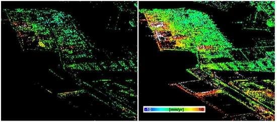
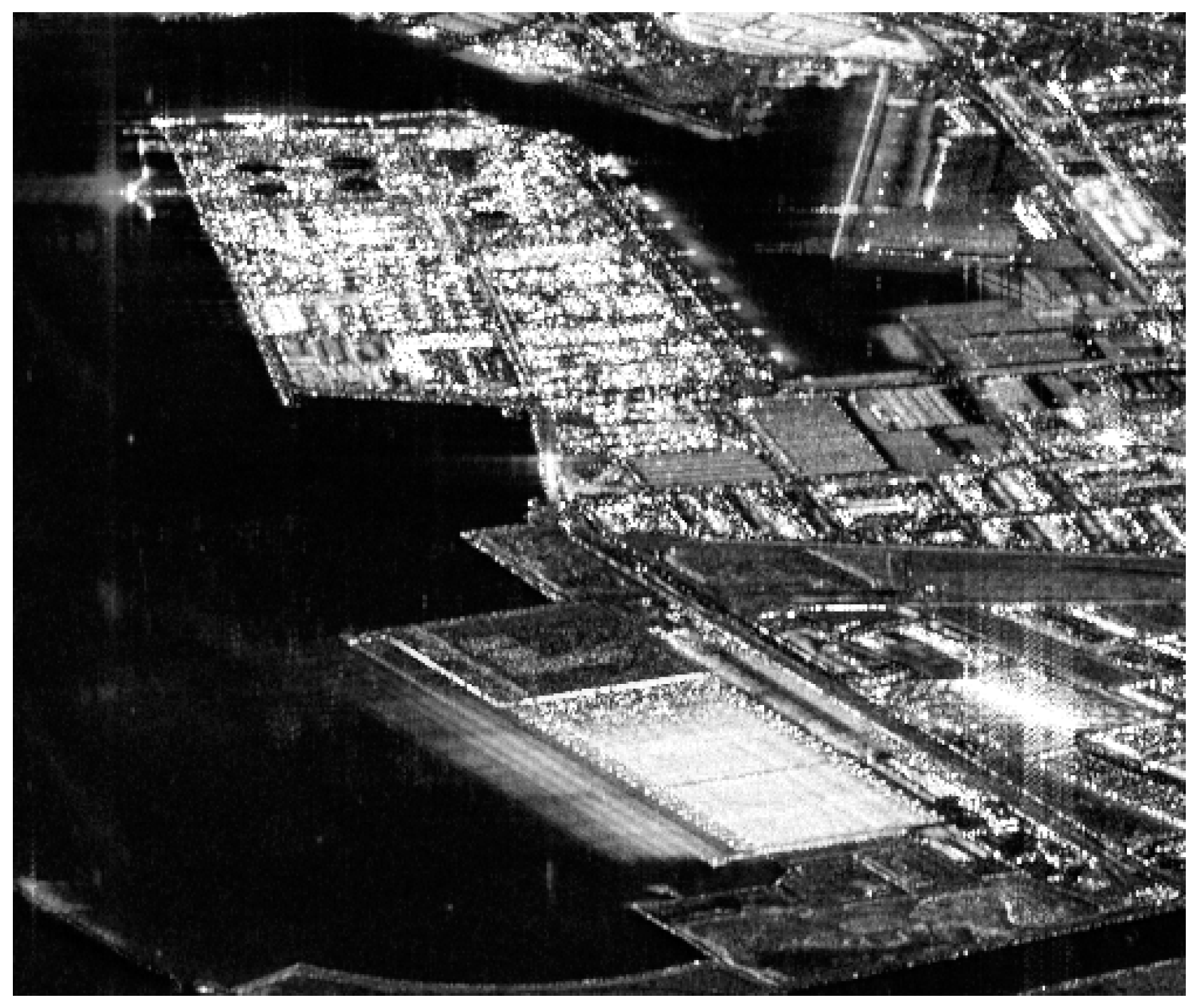
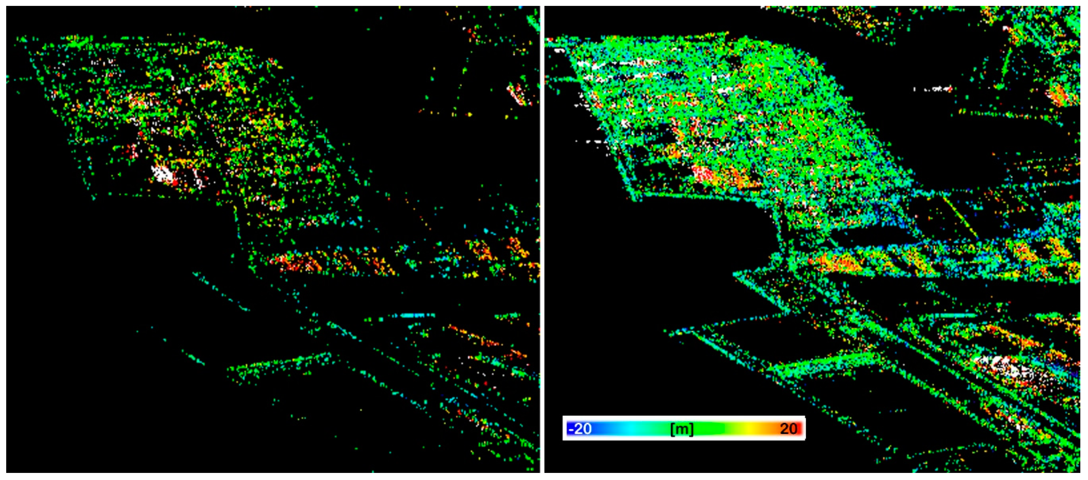
The first test area covers a part of the Port of Barcelona, see the amplitude image in
Figure 1. The extension of the area is approximately 1.6 by 4.9 km. The spatial density of the scatterers detected by PSI and the Fast-Sup-GLRT is shown in
Figure 2. The number of detected scatterers by the PSI approach is 8700, while over the same area, the number of scatterers detected by TomoSAR is 33,350. One may notice a remarkable difference in the measurements’ density: There is a factor 4 between the two solutions. Similar results are discussed in Reference [
29]. This is a direct consequence of the strategies used in the two data analyses. The PSI results were generated using an amplitude dispersion threshold of 0.2, followed by a threshold on the temporal coherence of the arcs of 0.7. For Fast-Sup-GLRT, the thresholds in Equation (6) were computed by Monte Carlo simulation for the considered system parameters and acquisition configuration and fixing
PFD =
PFA = 10
−5. For instance, for evaluating
T1, the Monte Carlo approach consists of simulating a large number of realizations of clutter plus noise signals, i.e., the data under hypothesis
H0. Then, for a given
PFA, the threshold is evaluated such that
with a probability equal to the fixed
PFA. Choosing
PFA = 10
−5 implies that we expect, on the first test area, a maximum number of false alarms equal to 2. A rough criterion for checking the adequacy of the chosen thresholds is the absence of detected scatterers on the sea area and the correct height positioning of the detected scatterers. Of course, when the thresholds decrease, the number of detected scatterers increases, with a possible precision degradation.
It is worth mentioning the different computational burden of the two techniques. Considering the main processing step, i.e., the estimation of the three model parameters for each selected scatterer, to process the same dataset using equivalent computational resources and the current implementation of the two techniques, TomoSAR takes approximately 60 times the time required by PSI. For this test site, the three-parameter PSI estimation takes approximately 40 min.
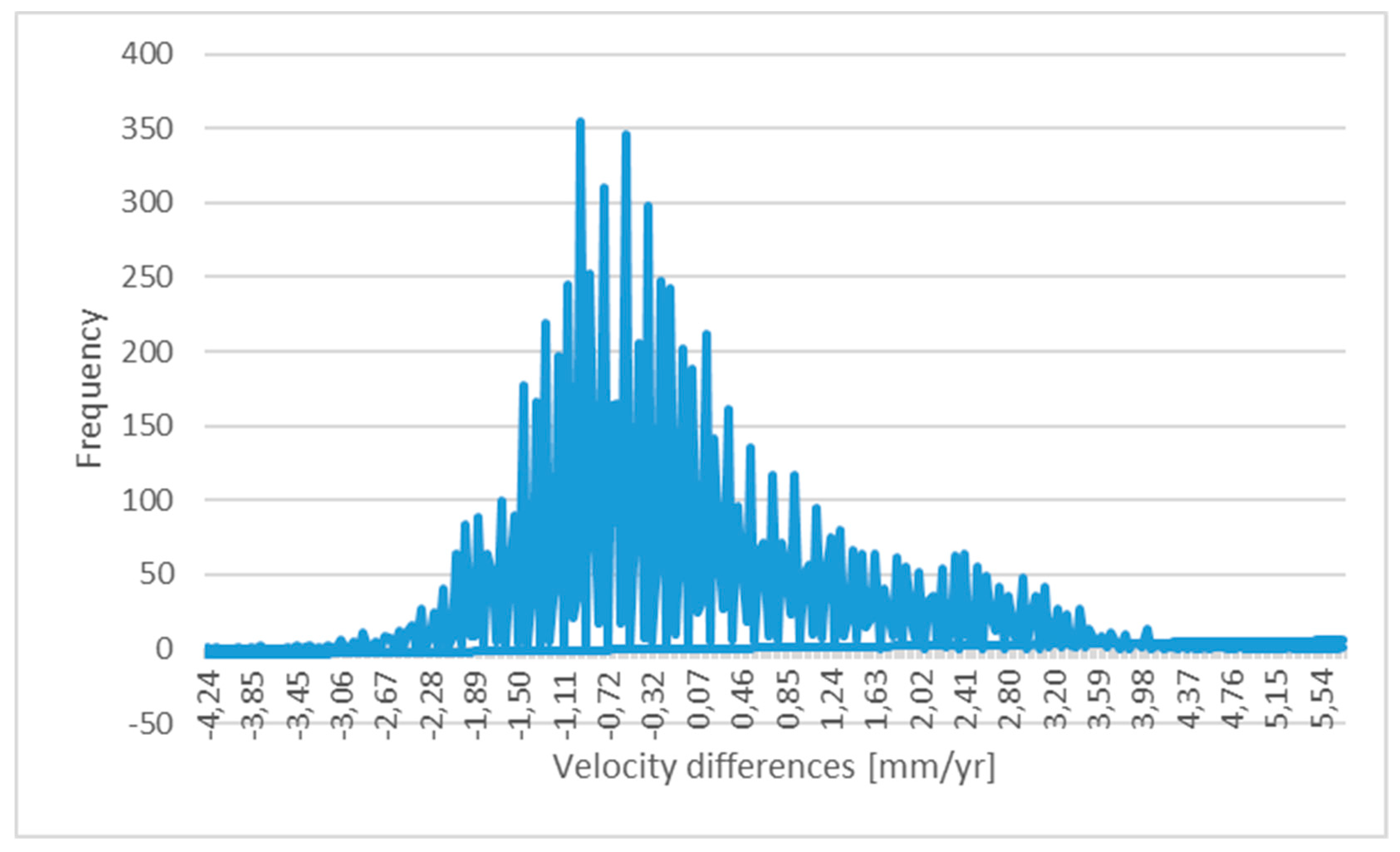
The intercomparison of the results of the two techniques was computed over the set of scatterers that is common to both techniques, which includes 8684 points. The statistics of the deformation velocity intercomparison, i.e., the statistics of the differences of the deformation velocity values, are shown in
Table 1, while the histogram of the velocity differences is shown in
Figure 3.
PSI and TomoSAR used the same reference point: The mean of the velocity differences indicates that there is basically no bias between the two experimental results. The most interesting parameter is given by the standard deviation of the velocity differences (1.36 mm/year): This indicates the dispersion of the population of the velocity differences. From this parameter, we can get valuable information on the standard deviation of the deformation velocity of each technique. For instance, by assuming the same precision for the two compared techniques and uncorrelated errors between the same techniques, it is possible to estimate the standard deviation of the deformation velocity of each technique as 1.36/√2 = 0.96 mm/year. The value 1 mm/year is often mentioned in the literature as the precision of the PSI deformation velocity, e.g., see Reference [
30]: In this case study, this value is confirmed.
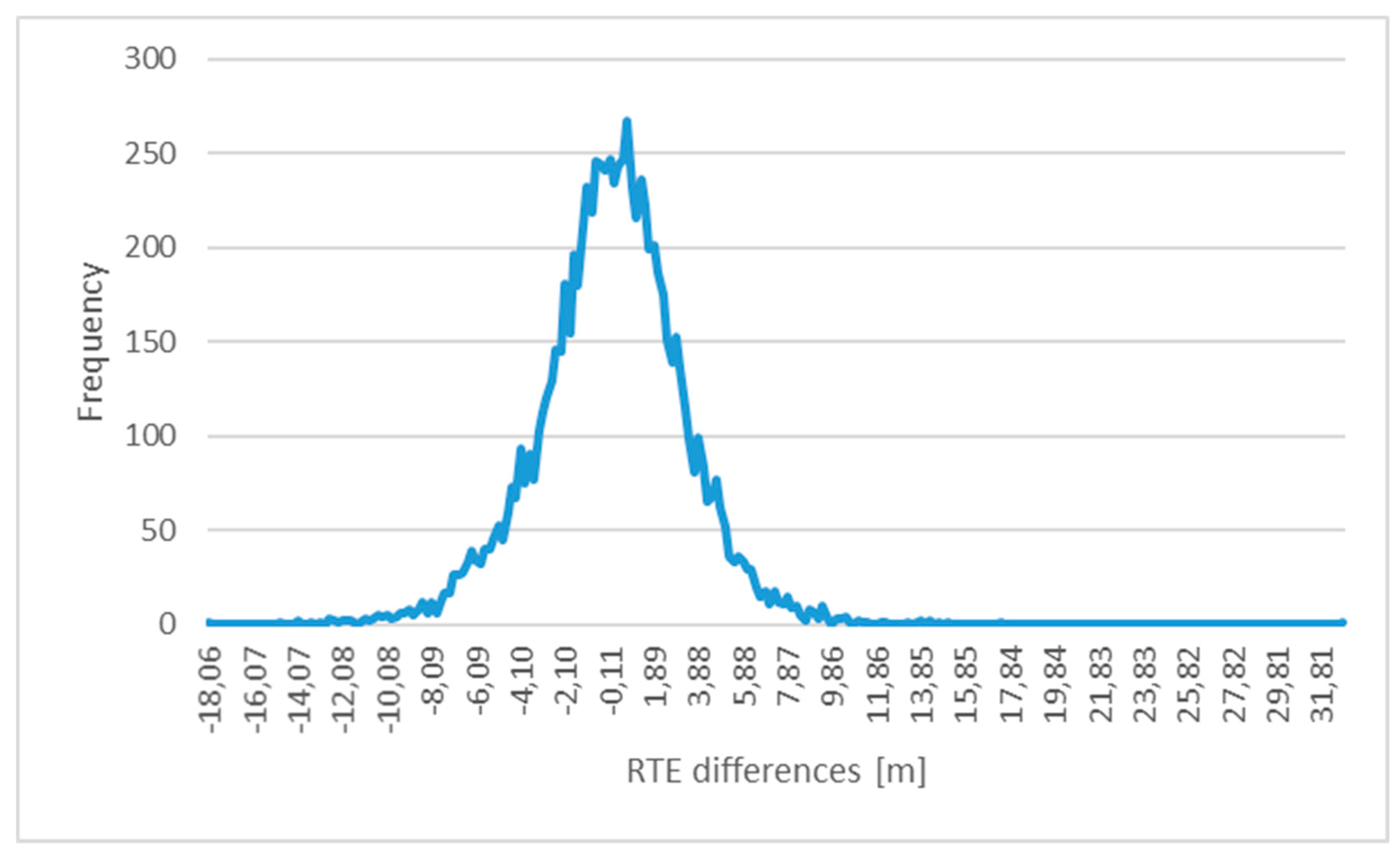
The same analysis was carried out for the RTE.
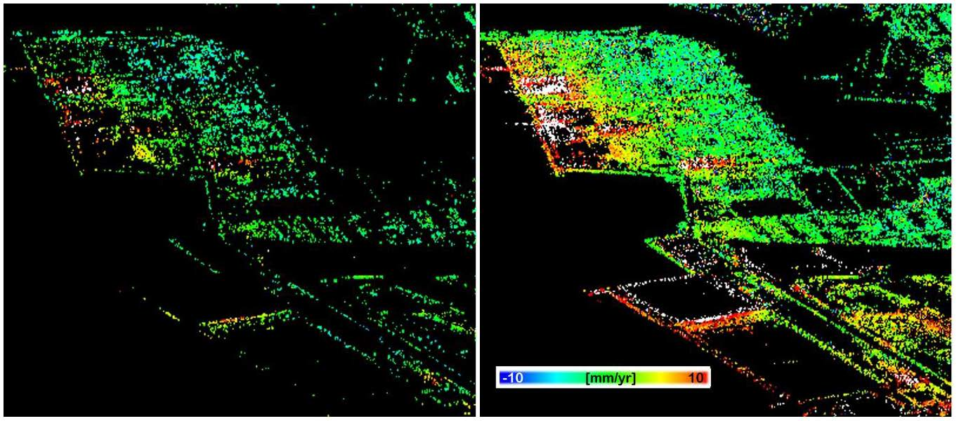
Figure 4 shows the RTE maps coming from PSI and TomoSAR. The main statistics of the differences are summarized in
Table 1, while the histogram of the differences is shown in
Figure 5. The mean difference is close to zero: There is a negligible bias between the two datasets. An interesting experimental parameter is given by the standard deviation of the RTE differences (3.25 m). Like in the case of the velocity, we can derive from this parameter the standard deviation of the RTE of each technique (PSI and TomoSAR): 2.3 m. This represents an interesting experimental result. In similar intercomparison exercises run using European Remote Sensing (ERS) and Envisat data, the same parameter was estimated to range between 0.9 and 2 m [
30]. From this case study, we can conclude that there is a relatively small impact of the reduced orbital tube of Sentinel-1 with respect to ERS and Envisat.
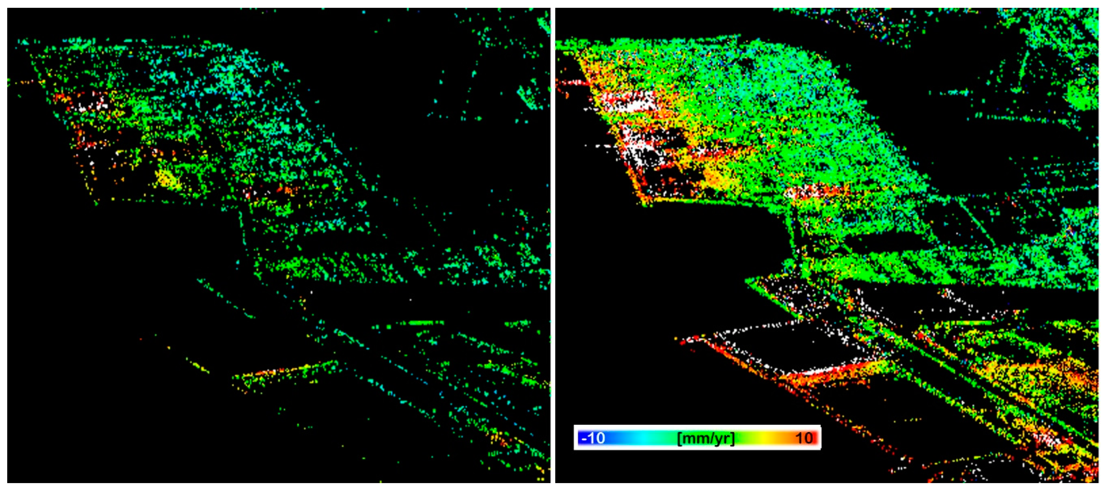
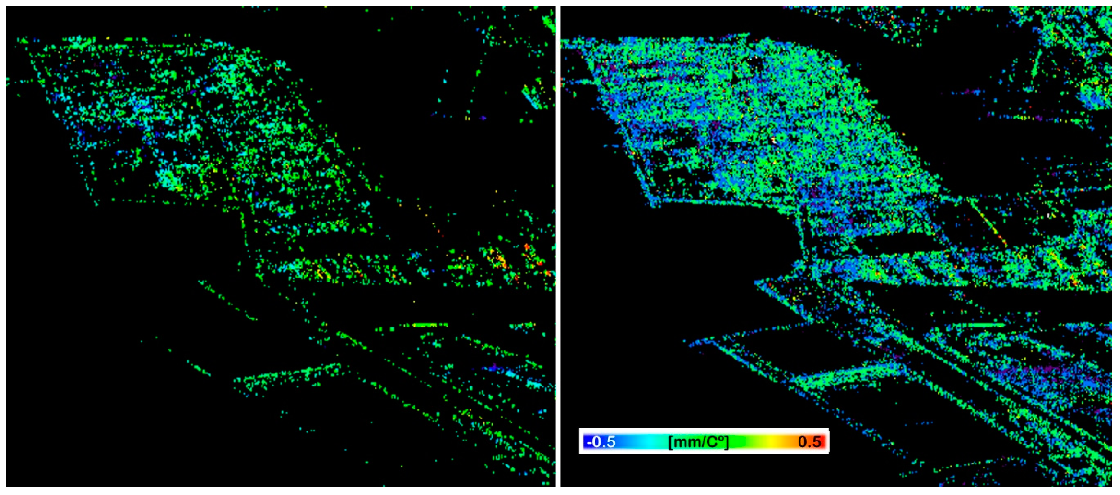
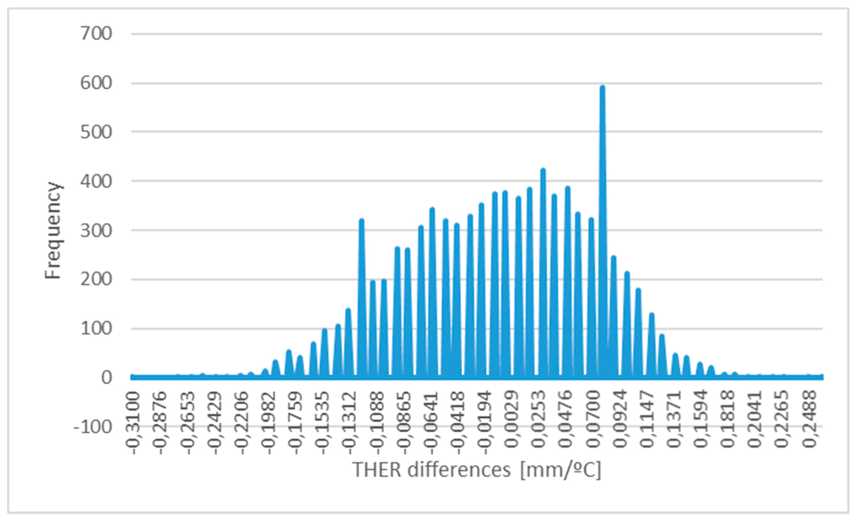
Finally, the analysis was focused on the THER parameter.
Figure 6 shows the THER maps coming from PSI and TomoSAR; the statistics of the intercomparison are shown in
Table 1, while the histogram of the THER differences is shown in
Figure 7. In this case, the mean difference is −0.005 mm/°C: This is a negligible bias, thanks to the fact that the datasets use the same reference point. The standard deviation of the THER difference (0.078 mm/°C) can be used to estimate the standard deviation of the THER estimated by each technique, obtaining the value of 0.055 mm/°C. This is an interesting experimental result, which is quite close to the value (0.04 mm/°C) derived using X-band data, which is described in Reference [
8].
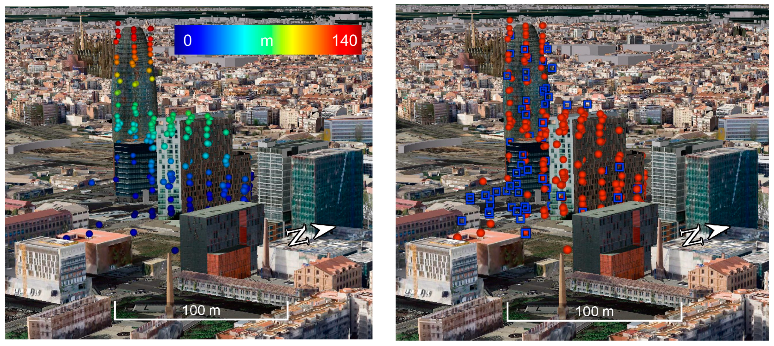
In this first case study, very few double scatterers were found using the TomoSAR processing. This is due to the relatively low height of the buildings and structures of this area: There are very limited layover areas, where the double scatterers are usually found. For this reason, we decided to include a second study area, which includes high-rise buildings. In this study area, we used the same SAR dataset of the first case study. The experiment focused on a small area (see
Figure 8), where TomoSAR found 427 single scatterers (red) and 178 double scatterers (blue), while PSI detected 172 single PSs. The common single scatterers are 166, while 6 of the 178 double scatterers coincide with single PSs. In
Figure 8, the location of doubles is explained by the presence of layover due to the Agbar tower (142 m) and to the neighboring building. Many points are on the ground and on the façade of Agbar tower and of the neighboring building. The majority of the 178 double scatterers (172) correspond to pixels that were discarded during the PSI pixel selection. Regarding the 6 PSs that are detected as double scatterers by TomoSAR, most probably, one of the two scatterers dominates with respect to the other one. For this reason, such scatterers are correctly selected by PSI, but their parameter estimates are slightly different from the ones provided by TomoSAR.
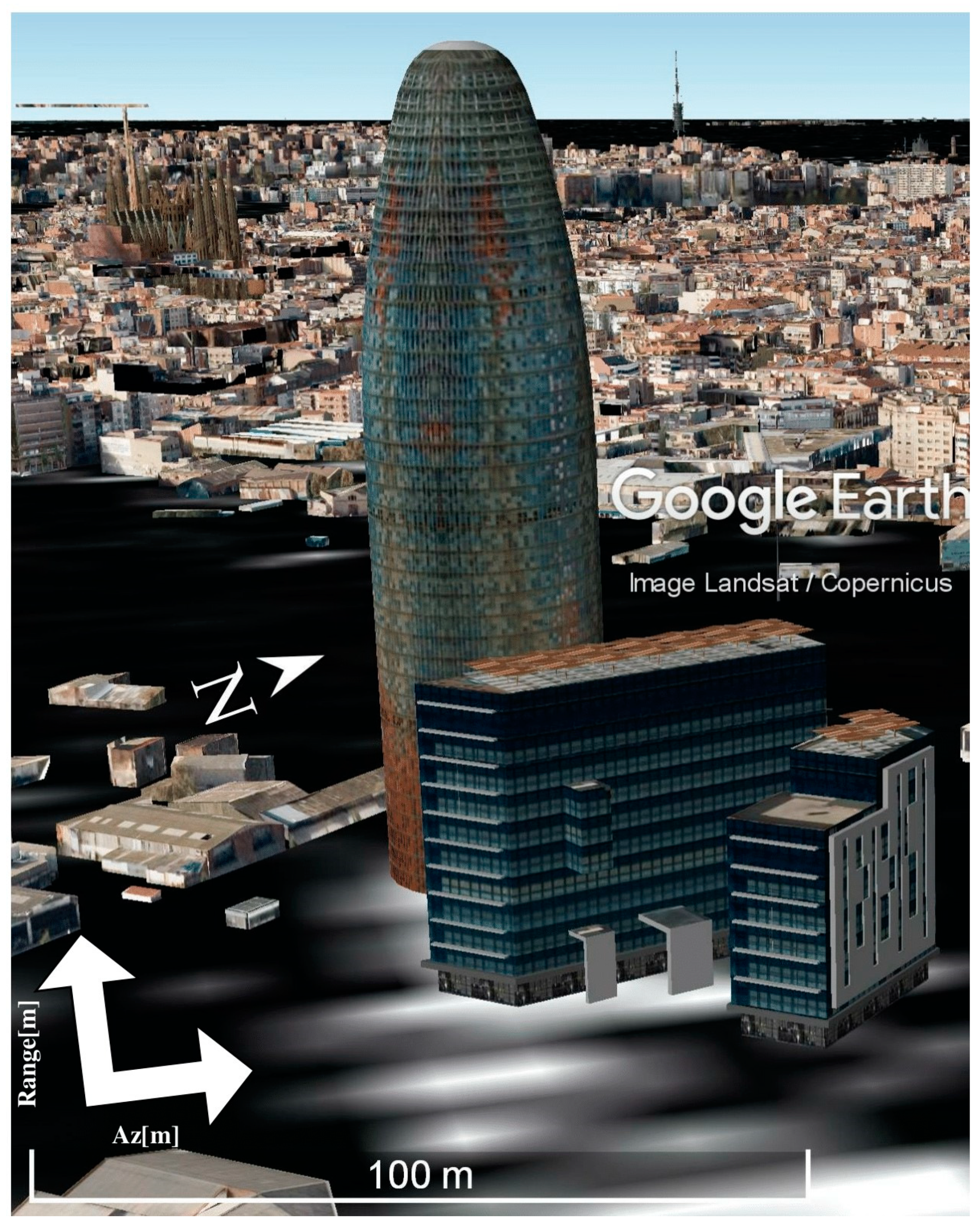
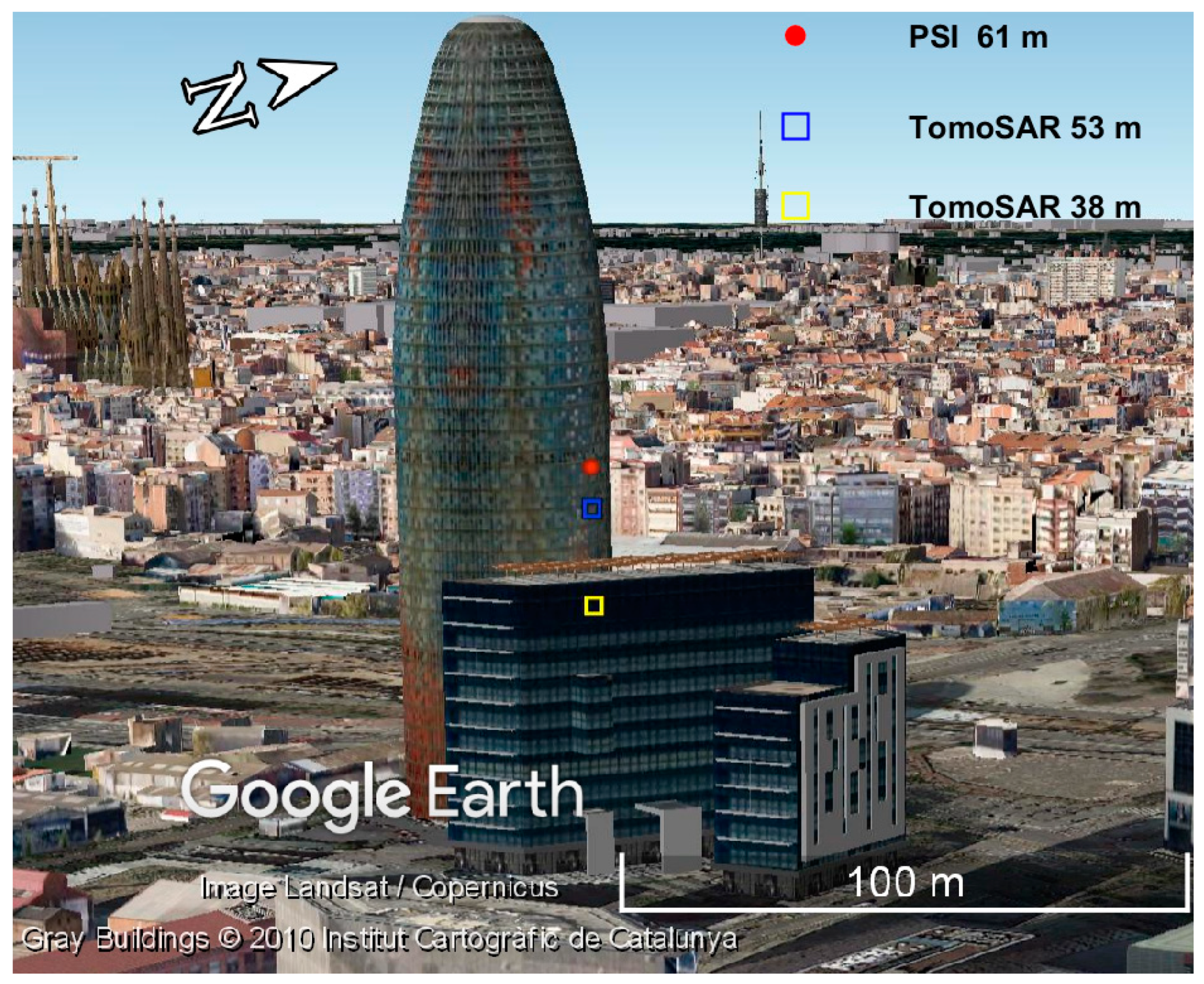
Figure 9 shows the range and azimuth direction and the layover area. As an example,
Figure 10 shows the localization of one of the six PS detected as a double scatterer by TomoSAR: PSI identifies only one scatterer with a height of 61 m, while TomoSAR identifies two scatterers with heights of 53 m and 38 m, respectively.
Summarizing, TomoSAR provides a larger set of single scatterers, which essentially includes all the scatterers detected by PSI, and additionally detects a significant number of double scatterers, which are mostly discarded by PSI. Then, TomoSAR allows the increase of the deformation measurement density, complementing PSI results and providing an added value.
5. Conclusions
In this paper, the TomoSAR applicability to Sentinel-1 data has been shown. An intercomparison of PSI and TomoSAR applied to Sentinel-1 data in order to monitor an urban area was carried out. The two techniques allow to estimate the following parameters over single and multiple scatterers: Height (RTE),linear deformation velocity (VELO), and the thermal expansion parameter (THER). Even if Sentinel-1 data have not been explicitly designed for tomography, in the two analyzed areas, the TomoSAR analysis has yielded good results, especially in terms of the high density of measurement points: The point density of TomoSAR is four times the density of the PSI results. The difference in the number of detected scatterers is mainly due to the coherent processing in the elevation direction of TomoSAR. By contrast, PSI processing is much less time consuming: For the same test area and similar computational resources, TomoSAR took approximately 60 times the time required by PSI.
The key experimental part of this work was devoted to the intercomparison of the PSI and TomoSAR results over two test areas. The most interesting results concern the standard deviations of the differences of the three main parameters (VELO, RTE, and THER), from which the standard deviation of each technique can be estimated. In terms of VELO, this corresponds to 0.96 mm/year for both PSI and TomoSAR. This is a value very close to 1 mm/year, which is often mentioned in the literature as the PSI precision of the deformation velocity. In terms of RTE, the standard deviation of the RTE of each technique (PSI and TomoSAR) is 2.3 m. This is an interesting experimental result, which is not so far from the values obtained in previous studies for ERS and Envisat (ranging between 0.9 and 2 m) [
30]. This result indicates that there is a relatively small impact of the reduced orbital tube of Sentinel-1 with respect to ERS and Envisat. Finally, in terms of THER, the standard deviation of each technique is 0.055 mm/°C: This result is quite close to the value (0.04 mm/°C) derived using X-band data in a previous study [
8].
If we consider the processing time, the PSI remains the reference technique, while TomoSAR can be used to complement the measurements done by PSI. This has been evidenced in the second case study of this work, considering the TomoSAR results in a layover area. Most of the detected double scatterers correspond to pixels that were discarded during the PSI pixel selection, which are useful to further increase the PSI deformation measurement density, providing an added value. However, if the processing time is not a major concern, TomoSAR can directly replace PSI.

 ,
, 


