Detection of Rice Phenological Variations under Heavy Metal Stress by Means of Blended Landsat and MODIS Image Time Series

Abstract

Monitoring phenological changes of crops through remote sensing methods is becoming a new perspective in assessing heavy metal contamination in agricultural farmlands. This paper proposes a method that combines the normalized difference vegetation index (NDVI) and the normalized difference water index (NDWI) to detect heavy metal stress-induced variations in satellite-derived rice phenology. First, we applied the enhanced spatial and temporal adaptive reflectance fusion model to obtain the NDVI and NDWI time series for the NDVI–NDWI phase–space construction. Then, six specific rice phenometrics were derived from the NDVI and the phase–space, respectively. Last, we introduced a relative phenophase index (RPI), which characterizes the relative change of the phenometrics to identify the rice paddies under heavy metal stress. The results indicated that satellite-derived rice phenometrics are generally influenced by human and natural factors (e.g., transplanting date, air temperature, and solar radiation), while the RPI showed weak correlations with all of these variables. In the determination of heavy metal stress, the NDVI- and phase–space-based RPIs of unstressed rice both show significantly (p < 0.001) higher values than those of stressed rice, while the phase–space-based RPI shows more apparent statistical difference between the stressed and unstressed rice compared to the NDVI-based one. Our work proved the capability of the phase–space-based method as well as the RPI in the discrimination of regional heavy metal pollution in rice fields.

1. Introduction

Heavy metal contamination in agricultural soil is one of the most severe problems affecting food security and public health at global and local levels [1]. Generally, pollution is caused against a backdrop of urban industrialization and is commonly characterized as relatively stable in spatial and temporal distribution [2,3]. A number of agronomy studies have exhibited the variations in spectral properties, pigment content, dry matter, photosynthesis, and transpiration of plants under heavy metal stress [4,5,6]. Based on these symptoms, researchers have made attempts to (1) extract the characteristics of multispectral and hyperspectral signatures [7,8,9]; (2) retrieve physiological and biochemical parameters [10,11]; and (3) integrate remote sensing data and crop growth models [12,13,14,15] to detect heavy metal contamination in agricultural soils.

Since satellite remote sensing has enabled the continuous monitoring of crop growth, it provides a new insight to indicate environmental interactions in agricultural systems through variations in crop phenology [16,17,18,19]. Heavy metals affect crop development mainly by interfering with physiological activity, and it has been observed that the onset of heading is delayed when rice is exposed to cadmium [4,6]. Basically, the change of the growth stages will certainly impact the vegetation index (VI) time series, thereby reflecting in the satellite-derived phenometrics. However, the detection of heavy metal stress-induced variations in rice phenology through the remote sensing approach is still problematic. One reason is the temporal mismatch between the satellite-derived rice phenometrics and the actual phenological events. Typically, a satellite-based phenometric is the certain date of a feature point on the VI curve, while an actual phenological event refers to a certain stage in rice development. Moreover, for rice agroecosystems, the absolute dates do not mean much in identifying the stress-induced change in the growth state, because they are mainly decided by the timing of transplanting. Liu et al. [20] analyzed the differences in the lengths of phenophases, which are defined as the period between two specific rice phenometrics, across a heavy metal stress gradient. However, the length of a phenophase may also be influenced by meteorological factors (e.g., air temperature and solar radiation), soil conditions, and management practices [21,22,23]. Therefore, more effort is needed to explore the relationships between the delaying of the actual heading stage and the variations of satellite-derived phenometrics under heavy metal stress.

Optical observations of crop phenology have mostly used greenness VIs, such as the normalized difference vegetation index (NDVI) and the enhanced vegetation index (EVI) [24,25,26,27]. However, they may not identify the greenness-independent features, such as canopy water content, which could also be sensitive to the phenophase transition. The normalized difference water index (NDWI) has also been used to characterize the phenological cycle of vegetation—however, mostly for reducing the effect of snow in boreal natural ecosystems [28,29,30]. In addition to a single-purpose VI, Gonsamo et al. [31] combined the advantages of NDVI and NDWI to detect vegetation phenology with the small effect of soil and snow. Likewise, Thompson et al. [32] derived phenometrics in a seasonally snow-covered landscape using a phase–space diagram, which was constructed by the NDVI–NDWI time series over an entire phenological year. The observed pixels in the phase–space were segmented into snow-covered and snow-free phases by K-means clustering, which made the phenological descriptors (e.g., start of the growing season) free of the influence of the onset/offset of snow. Moreover, Ding et al. [33] explored the EVI- and NDWI-based autumn phenology in semi-arid grasslands and proved that the phenometrics derived from NDWI, which represents the metabolic activity of vegetation, was generally later than that from EVI, which stands for the photosynthetic activity. Since stress and disturbance could impact not only photosynthesis but also the whole physiological function of the plant, the greenness–wetness synergetic strategy possessed an advantage in comprehensively characterizing the subtle variation of canopy components in vegetation growth [34,35,36].

The main objectives of this paper are to (1) create an NDVI–NDWI phase–space for the rice growth season using fused Landsat and MODIS image times series; (2) derive six specific satellite-based phenometrics: Active tillering date ($D_{til}$), middle heading date ($D_{head}$), maturity date ($D_{mat}$), growth season length ($L_{season}$), vegetative phase length ($L_{veg}$), and reproductive phase length ($L_{rep}$) based on NDVI time series and phase–space, respectively; and (3) perform a relative phenophase index (RPI) to discriminate rice fields under heavy metal stress from unstressed ones.

2. Materials and Methods

2.1. Study Area

The study area is situated in Zhuzhou City, Hunan Province (Figure 1). This area is a region of a subtropical monsoon climate characterized by hot and wet summers with sufficient sunlight for rice growth. The mean annual temperature ranges from 16 to 18 ${}^{\circ }$C. The mean annual precipitation is over 1400 mm. The predominant soil type is orthic acrisol according to the world reference base (WRB) for soil resources [37]. Zhuzhou is a commodity grain production base of China. The main crop type in Zhuzhou is paddy rice, and the predominant variety is Boyou9083, usually transplanted in early June and harvested in late September. Meanwhile, Zhuzhou is also an important industrial city with significant heavy metal pollution. Industrial waste is discharged into the Xiangjiang River, the most polluted river in China, and has large contaminated areas of land along the river. The rice in this region is cultivated in an intensive pattern as follows: The planted rice in the experimental sites is supplied with abundant irrigation water and the right amount of fertilizers and farm chemicals to prevent unwanted stress, including diseases, pests, and water and nutrition deficiency. Thus, heavy metals become the dominant stressors interfering with the growth of rice.

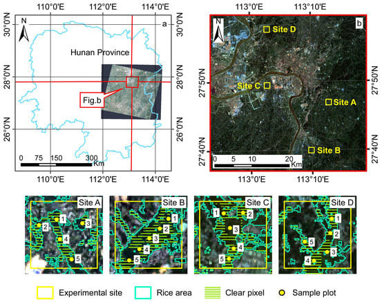
Figure 1. Location of the experimental sites in Zhuzhou, Hunan Province, China, and the spatial distribution of sample plots.

Four experimental sites, labeled A, B, C and D, were selected to account for differences in the severity of heavy metal stress (Figure 1b). Each of them had a size of 1.5 km × 1.5 km. The concentrations of cadmium (Cd), mercury (Hg), lead (Pb), and arsenic (As), which are the main pollutants in Hunan Province, were measured in the soil of all experimental sites (Table 1). In Sites B, C, and D, the concentrations of Cd, Hg, and Pb were all higher than background values and the concentration of Cd was significantly greater than the upper limit value of the National Secondary Standard in the Environment Quality Standard for Soils (GB15618-1995). According to the concentration of Cd, which was considered the main pollutant in the study area, Site A is categorized as “nonstress”, Site B is categorized as “moderate stress”, and Sites C and D are categorized as “severe stress”.

Table 1. The average condition of heavy metal contamination in the soil of the experimental sites.

Experimental	Geographic	Cd	Hg	Pb	As	Stress
Site	Coordinates					Level
A	27°47′ N 113°10′ E	0.84	0.35	78.33	10.23	Nonstress
B	27°40′ N 113°10′ E	2.31	0.24	91.05	17.34	Moderate stress
C	27°50′ N 113°02′ E	3.28	0.51	120.75	18.15	Severe stress
D	27°58′ N 113°02′ E	3.57	0.50	130	14.7	Severe stress
Background value		1.43	0.20	82.78	19.11
National secondary		0.3∼1.0	0.3∼1.0	250∼350	20∼30
standard

Note: Heavy metal concentrations are given in mg $·$ kg${}^{-1}$. The background data were acquired from the Hunan Institute of Geophysical and Geochemical Exploration, China. The heavy metals content was measured by the Analysis and Test Center, Institute of Environment and Sustainable Development in Agriculture, Chinese Academy of Agricultural Sciences (CAAS).

2.2. Data Collection

2.2.1. Field Measurements

Field experiments were performed from July to September, 2014. A total of 20 sample plots (five at each site) were set, of which each plot was 30 m × 30 m in size. All sample plots were georeferenced by a global positioning system instrument. Samples of soil were collected consistently in every sample plot and preserved in plastic bags. The sampling position was at the rooting zone and the sampling depth was 20 cm. The soil samples from the same sites were grouped together, dried at room temperature, ground, and then sent to the laboratory for physicochemical characteristics analysis. The measured values of each sample plot are presented in Table 1. Information on the critical growth periods of rice, including transplanting and harvesting date and tillering, heading, and maturity stage was collected for the 10 plots in Sites A and B by interviewing rice farmers. The plot-based rice growth stages were recorded as reference data and the NDVI- and phase–space-based phenometrics for the 10 corresponding pixels on the image were extracted.

2.2.2. Remote Sensing Images

We acquired the MODIS MOD09A1 product to obtain 8-day composite surface reflectance data with a spatial resolution of 500 m and the Landsat Level-2 product to acquire surface reflectance at 30-m spatial resolution. All available data for the study area between day of year (DOY) 137 (early May) and DOY 305 (late October) from 2013 to 2017 were collected (Figure 2). Remote images with the experimental sites fully covered by the cloud were excluded from analysis. The MOD09A1 product provides bands 1–7, of which band 3, band 4, band 1, band 2, and band 6 were selected as blue, green, red, NIR, and SWIR bands, respectively, while the Operational Land Imager (OLI) on Landsat 8 provides nine spectral bands, of which band 2, band 3, band 4, band 5, and band 6 were selected as blue, green, red, near infrared (NIR), and shortwave infrared (SWIR) bands, respectively (Table 2). Basic processing, including radiometric correction and geometric correction, was implemented in both products mentioned above to provide application-ready datasets. The Landsat 8 image on DOY 205 in 2016 was used to obtain the spatial distribution of rice using a supervised classification.

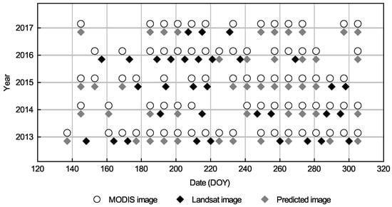
Figure 2. Scene acquisition dates by year for the Landsat, MODIS, and enhanced spatial and temporal adaptive reflectance fusion model (ESTARFM)-predicted images.

Table 2. Brief characteristics of LANDSAT 8- and MODIS-selected bands.

Band Name	Landsat 8				MOD09A1
	Band No.	Wavelength ($\mathsf{\mu }$m)	Resolution (m)		Band No.	Wavelength ($\mathsf{\mu }$m)	Resolution (m)
Blue band	Band 2	0.450–0.510	30		Band 3	0.459–0.479	500
Green band	Band 3	0.530–0.590	30		Band 4	0.545–0.565	500
Red band	Band 4	0.640–0.670	30		Band 1	0.620–0.670	500
NIR band	Band 5	0.850–0.880	30		Band 2	0.841–0.876	500
SWIR band	Band 6	1.570–1.650	30		Band 6	1.628–1.652	500

2.2.3. Auxiliary Data

Meteorological data, including the daily actual duration of sunshine and daily average air temperature from 2013 to 2017, were downloaded from the China Meteorological Data Sharing Service System (http://www.cma.gov.cn/). The solar radiation was calculated using the following equation [38]:

$$Rs=\left(a+b\frac{n}{N}\right)Ra,$$

(1)

where $Rs$ is the total daily solar radiation (J $·$ m${}^{-2}$), a and b are empirical constants of 0.25 and 0.5, n represents the daily actual duration of sunshine, N represents the daily potential duration of sunshine, and $Ra$ represents the extraterrestrial solar radiation (W $·$ m${}^{-2}$), which was calculated according to the method of Liu [39].

2.3. NDVI–NDWI Phase–Space Construction

High spatiotemporal resolution remote sensing data are essential in order to detect the slight changes in rice development caused by heavy metal stress. We used the enhanced spatial and temporal adaptive reflectance fusion model (ESTARFM) [40] to obtain a time series of the 8-day surface reflectance product (30 m) by blending the selected bands of Landsat 8 and MODIS data. ESTARFM focuses on improving data fusion for the mixed pixels and has made significant improvements in the accuracy of predictions for heterogeneous landscapes, which exist widely in our study area [41]. The ESTARFM algorithm uses two pairs of Landsat-MODIS images (i.e., dates $t_1$ and $t_3$) and one MODIS image (date $t_2$) to predict a Landsat-like image at date $t_2$. In this study, a total of 79 fine-resolution images (including 46 predicted images and the 33 original Landsat images) were obtained (Figure 2). We applied cloud and cloud shadow masks generated from the pixel quality assurance in the Landsat product to all synthetic images and removed them from the overall analysis.

NDVI, which is correlated with the absorption of photosynthetically active radiation, was calculated as follows [42]:

$$NDVI=\frac{{\rho }_{NIR}-{\rho }_{Red}}{{\rho }_{NIR}+{\rho }_{Red}},$$

(2)

where ${\rho }_{NIR}$, ${\rho }_{Red}$ and ${\rho }_{Blue}$ are the reflectances of the NIR band, red band, and blue band, respectively. NDWI, which is correlated with the canopy water content, was calculated as follows [43]:

$$NDWI=\frac{{\rho }_{NIR}-{\rho }_{SWIR}}{{\rho }_{NIR}+{\rho }_{SWIR}},$$

(3)

where ${\rho }_{SWIR}$ is the reflectance of the SWIR band.

The application of satellite-derived VI time series is inevitably hindered by noise arising from clouds, ozone, dust, and other aerosols. Though the cloud-polluted pixels were masked out, radiance disturbance still existed in the VI time series. To solve this problem, the VI time series were fitted using a double-logistic curve as follows [44]:

$$v\left(t\right)=a+b\left(\frac{1}{1+e^{ct+d}}+\frac{1}{1+e^{et+f}}\right),$$

(4)

where $v\left(t\right)$ represents the value at time t (d), and a, b, …, f are the fitting parameters. The daily NDVI and NDWI time series that covered the rice growth season (from DOY 120 to DOY 305) were then generated by the fitting function (Equation (4)). We gave an example of phase–space established by the greenness and wetness VI, of which the greenness VI takes the NDVI as an example and the wetness VI refers to the NDWI (Figure 3). In the NDVI–NDWI phase–space, the temporal trajectory of a rice pixel throughout the whole growth period first drifts towards the top right areas and then towards the bottom left areas with the progression. The dynamic of the pixel was described as $dist$, the distance from the pixel to the origin in the phase–space, by the following equation:

$$dist=\sqrt{NDV{I}^2+NDW{I}^2}.$$

(5)

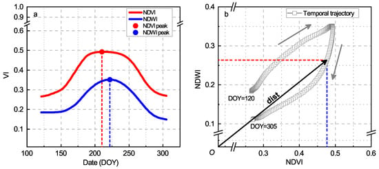
Figure 3. Schematics showing (a) the normalized difference vegetation index (NDVI) and normalized difference water index (NDWI) time series in date-VI form and (b) the calculation of $dist$ (the distance from the pixel to the origin in the phase–space) in the corresponding NDVI–NDWI phase–space for an example rice pixel.

2.4. Defining NDVI- and Phase–Space-Based Rice Phenometrics

The active tillering date ($D_{til}$), middle heading date ($D_{head}$), and maturity date ($D_{mat}$) were first defined for the NDVI time series: The date of the maximum point on the first derivative was used to estimate $D_{til}$; the date of the maximum point was used to estimate $D_{head}$; and the date of the minimum point on the first derivative was used to estimate $D_{mat}$ (Figure 4a) [24,45,46]. Then, we applied these existing phenological extraction methods to the phase–space. Specifically, the phenometrics were redefined based on the time series of dist: $D_{til}$ was redefined as the date of the maximum point on the first derivative of $dist$; $D_{head}$ was redefined as the date of the maximum value of $dist$ and $D_{mat}$ was redefined as the date of the minimum point on the first derivative of $dist$ (Figure 4b).

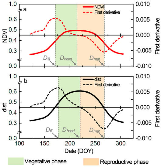
Figure 4. Temporal profiles and the first derivatives of NDVI (a) and $dist$ (b). The vertical dashed lines refer to the dates of active tillering ($D_{til}$), middle heading ($D_{head}$), and maturity ($D_{mat}$), from left to right.

Since soil-related factors (e.g., soil moisture) greatly impact the VI values in the early growth period of rice (i.e., from transplanting to active tillering) due to the low vegetation cover, we prefer to set the growth season of interest to start at active tillering instead of transplanting. As the heading stage was supposed to divide rice development into vegetative and reproductive growth [45,47,48], we defined the vegetative phase as the period from $D_{til}$ to $D_{head}$ and the reproductive phase as the period from $D_{head}$ to $D_{mat}$. Thus, another three phenometrics, growth season length ($L_{season}$), vegetative phase length ($L_{veg}$), and reproductive phase length ($L_{rep}$), were calculated as follows:

$$L_{season}=D_{mat}-D_{til},$$

(6)

$$L_{veg}=D_{head}-D_{til},$$

(7)

$$L_{rep}=D_{mat}-D_{head},$$

(8)

where $L_{season}$, $L_{veg}$, and $L_{rep}$ represent the lengths of growth season, vegetative phase, and reproductive phase (d), respectively. Particularly, the NDVI-based $L_{season}$, $L_{veg}$, and $L_{rep}$ were calculated by the NDVI-based $D_{til}$, $D_{head}$, and $D_{mat}$, while the phase–space-based $L_{season}$, $L_{veg}$, and $L_{rep}$ were calculated by the phase–space-based $D_{til}$, $D_{head}$, and $D_{mat}$.

2.5. Relative Phenophase Index (RPI)

To evaluate heavy metal stress-induced satellite-derived rice phenometrics, a relative phenophase index was then defined as:

$$RPI=\frac{L_{rep}-L_{veg}}{L_{rep}+L_{veg}},$$

(9)

where $L_{veg}$ and $L_{rep}$ represent the lengths of the vegetative and reproductive phase, respectively. The RPI characterizes the difference between the vegetative and reproductive phase durations relative to the growth season. Based on the relationships between satellite-based phenometrics and the actual rice growth stages, the delaying of the heading stage caused by heavy metal stress could also result in a time lag of the $D_{head}$, and thus a relative change of $L_{veg}$ and $L_{rep}$. Therefore, the RPI for the stressed rice paddies would theoretically exhibit a lower value due to the relative longer vegetative phase. We developed NDVI- and phase–space-based RPI, computed based on NDVI- and phase–space-based phenometrics, respectively, for a comparison in the subsequent analyses.

2.6. Statistical Analysis

Crop phenology is considered a function of accumulated degree days, photoperiod, and vernalization requirements [49]. Specifically, a settled level of the temperature or solar radiation accumulation would shift the crop growth cycle from one stage to the next stage. As the goal of this study was to detect the stress-induced phenological characteristics, the meteorological variables should be taken into account as interferences. We used partial correlation analysis and significance tests to evaluate the influence of the meteorological variability on $L_{season}$, $L_{veg}$, $L_{rep}$, and the RPI. The daily mean air temperature of the growth season ($T_{season}$), the vegetative phase ($T_{veg}$) and the reproductive phase ($T_{rep}$) and the daily mean solar radiation of the growth season ($R{s}_{season}$), the vegetative phase ($R{s}_{veg}$), and the reproductive phase ($R{s}_{rep}$) were calculated for each year of the period 2013–2017. To test the null hypothesis that the RPI was not significantly different between experimental sites, a standard analysis of variance (ANOVA) was conducted using a significance level of 0.001. The post-hoc test (Dunnett’s T3) was applied to determine significant differences between any two of the four study sites at p < 0.001.

3. Results

3.1. Validation of Satellite-Derived Phenometrics with Field Investigation

The transplanting date, tillering stage, heading stage, maturity stage, and harvesting date (the end of the maturity stage) acquired from the field survey are shown in Figure 5. The lengths of the actual growth season (from transplanting date to harvesting date) were nearly the same for the 10 sample plots. The timing of transplanting was generally earlier in Site A (from DOY 148 to DOY 153) than in Site B (from DOY 154 to DOY 160), which caused the whole growth season of rice paddies in Site B to lag behind those in Site A. We chose to qualitatively validate the derived phenometrics with the survey data. Specifically, the satellite-derived $D_{til}$, $D_{head}$, and $D_{mat}$ were validated against the stages of tillering, heading, and maturity collected by field survey. The NDVI- and phase–space-based phenometrics all lay within the corresponding rice growth stage, which indicated that satellite-derived phenometrics are reasonable.

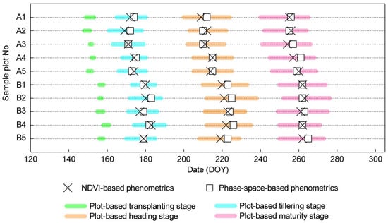
Figure 5. Comparison between satellite-derived rice phenometrics and plot-based rice growth stages for Site A and B in 2014. The satellite-derived phenometrics include the dates of active tillering ($D_{til}$), middle heading ($D_{head}$), and maturity ($D_{mat}$), from left to right, derived from NDVI and phase–space, respectively. The rice phenological stages from the 10 sample plots were acquired from the in-situ investigations. The end of the maturity stage represents the harvesting date.

3.2. Comparison of the Spatial Variability of Phenometrics

The spatial distributions of mean $D_{til}$, $D_{head}$, and $D_{mat}$ for Sites A and B during the period 2013–2017 are presented in Figure 6. Generally, all of these three phenometrics in Site A were earlier than those in Site B. For either the NDVI- or the phase–space-based phenometrics, the overall mean $D_{til}$ and $D_{head}$ in Site A were approximately 5–7 days earlier than those in Site B, while the overall mean $D_{mat}$ in Site A was only 2–3 days earlier than that in Site B. The NDVI- and the phase–space-based phenometrics were close to each other. For both experimental sites, the overall mean values of NDVI-based $D_{til}$ and $D_{head}$ were 1–3 days earlier than those based on phase–space, while the overall mean values of NDVI-based $D_{mat}$ were almost the same or a little later (approximately 1 day) compared to the phase–space-based ones.

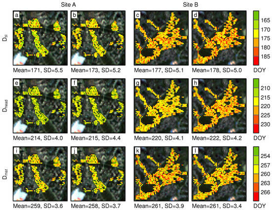
Figure 6. Spatial distributions of the mean dates of active tillering ($D_{til}$) (a–d), middle heading ($D_{head}$) (e–h), and maturity ($D_{mat}$) (i–l) for Sites A and B during the period 2013–2017. Each of the phenometrics was derived from NDVI (a,c,e,g,i,k) and phase–space (b,d,f,h,j,l).

The spatial distributions of the mean $L_{season}$, $L_{veg}$, and $L_{rep}$ in Sites A and B during the period 2013–2017 are presented in Figure 7. For either the NDVI- or the phase–space-based phenometrics, the overall mean $L_{season}$ and $L_{rep}$ in Site A were 2–3 days longer than those in Site B, while the overall mean $L_{veg}$ in Site A was 1–2 days shorter than that in Site B. For both experimental sites, the overall mean values of the NDVI-based $L_{season}$ and $L_{rep}$ were 1–2 days longer than those derived from the phase–space, while the overall mean values of NDVI-based $L_{veg}$ were the same or a little longer (1 day) compared to the phase–space-based ones. Noticeably, the spatial standard deviations of the 5-year mean $L_{season}$ (2.8 to 3.1), $L_{veg}$ (2.0 to 2.4), and $L_{rep}$ (1.9 to 2.2) were distinctly smaller than those of the 5-year mean $D_{til}$ (5.0 to 5.5), $D_{head}$ (4.0 to 4.4), and $D_{mat}$ (3.4 to 3.9).

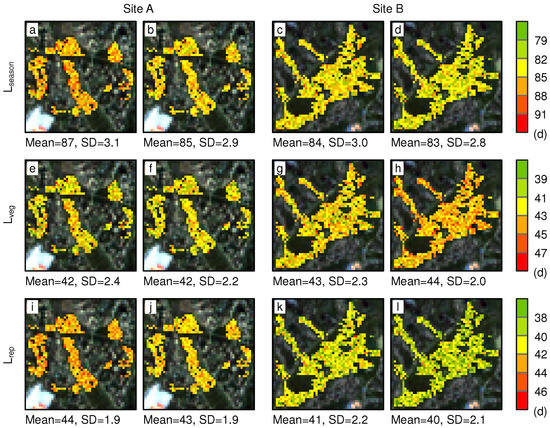
Figure 7. Spatial distributions of the mean lengths of growth season ($L_{season}$) (a–d), vegetative phase ($L_{veg}$) (e–h), and reproductive phase ($L_{rep}$) (i–l) for Sites A and B during the period 2013–2017. Each of the phenometrics was derived from NDVI (a,c,e,g,i,k) and phase–space (b,d,f,h,j,l).

3.3. Influence of Meteorology on Phenometrics and the RPI

Table 3 shows the partial correlation coefficients between the phenometrics and the meteorological factors in the four study sites. $L_{season}$, $L_{veg}$, and $L_{rep}$ were all significantly (p < 0.001) correlated (negatively) with the daily mean air temperature during the corresponding period. For both of the NDVI- and phase–space-based phenometrics, $L_{season}$ and $L_{veg}$ showed moderate correlations ($-0.55$ < r < $-0.45$) with the $T_{season}$ and $T_{veg}$, respectively, while $L_{rep}$ showed weak correlations ($-0.34$ < r < $-0.33$) with the $T_{rep}$. Similarly, $L_{season}$, $L_{veg}$, and $L_{rep}$ were significantly (p < 0.001) correlated (negatively) with the daily mean solar radiation during the corresponding period. For both of the NDVI- and phase–space-based phenometrics, $L_{season}$ and $L_{veg}$ showed moderate correlations ($-0.55$ < r < $-0.40$) with the $R{s}_{season}$ and $R{s}_{veg}$, respectively, while $L_{rep}$ showed weak correlations ($-0.31$ < r < $-0.29$) with the $R{s}_{rep}$.

Table 3. Partial correlation coefficients between derived phenometrics and meteorological factors calculated based on the period of the corresponding phenometrics for all pixels in the four experimental sites during the period 2013–2017. ** p-value statistically significant at <0.001.

	NDVI-Based Phenometrics				Phase–Space-Based Phenometrics
	${\mathit{L}}_{\mathit{season}}$	${\mathit{L}}_{\mathit{veg}}$	${\mathit{L}}_{\mathit{rep}}$		${\mathit{L}}_{\mathit{season}}$	${\mathit{L}}_{\mathit{veg}}$	${\mathit{L}}_{\mathit{rep}}$
$T_{season}$	$-0.48$ **				$-0.45$ **
$T_{veg}$		$-0.55$ **				$-0.54$ **
$T_{rep}$			$-0.34$ **				$-0.33$ **
$R{s}_{season}$	$-0.42$ **				$-0.40$ **
$R{s}_{veg}$		$-0.55$ **				$-0.54$ **
$R{s}_{rep}$			$-0.31$ **				$-0.29$ **

By contrast, the RPI showed generally weak or nonsignificant correlations with the meteorological variables (Table 4). The NDVI-based RPI showed stronger correlations ($-0.30$ < r < $-0.08$) with the daily mean air temperature and the daily mean solar radiation compared to the phase–space-based one ($-0.26$ < r < $-0.01$). The correlations between the RPI and meteorological factors during the vegetative phase were relatively stronger ($-0.26$ and $-0.21$).

Table 4. Partial correlation coefficients between the relative phenophase index (RPI) and meteorological factors calculated based on the period of the corresponding phenometrics for all pixels in the four experimental sites during the period 2013–2017. ** p-value statistically significant at <0.001.

	NDVI-Based RPI	Phase–Space-Based RPI
$T_{season}$	$-0.19$ **	$-0.15$ **
$T_{veg}$	$-0.30$ **	$-0.26$ **
$T_{rep}$	$-0.10$	$-0.08$
$R{s}_{season}$	$-0.17$ **	$-0.09$
$R{s}_{veg}$	$-0.27$ **	$-0.21$ **
$R{s}_{rep}$	$-0.08$	$-0.01$

3.4. Regional Heavy Metal Stress Detection

The spatial and frequency distributions of RPI in the four experimental sites are presented in Figure 8 and Figure 9. The NDVI-based RPI was calculated by the mean $L_{veg}$ and $L_{rep}$ derived from NDVI, while the phase–space-based RPI was calculated by the mean $L_{veg}$ and $L_{rep}$ derived from the phase–space during the period 2013–2017. Generally, (1) RPI values for Site A (nonstress) were greater than those for Sites B, C and D (stress); (2) for stressed sites, the RPI for Site B (moderate stress) was greater than those for Sites C and D (severe stress); (3) RPIs for Sites C and D were close to each other. According to the statistical results, both the NDVI- and phase–space-based RPI showed significant (p < 0.001) difference across the heavy metal stress gradient (Table 5). Compared to the NDVI-based RPI, the phase–space-based RPI showed a more obvious difference under different stress levels according to the overlapping proportion (Figure 9).

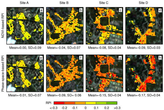
Figure 8. Spatial distributions of the mean values of (a–d) the NDVI-based RPI and (e–h) the phase–space-based RPI during the period 2013–2017.

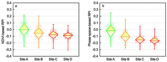
Figure 9. Statistical box charts of (a) the NDVI-based RPI and (b) the phase–space-based RPI in the four experimental sites. Central lines represent the medians, boxes represent mean ± standard deviation, and the whiskers represent the minimum and maximum values.

Table 5. Sensitivity of the NDVI- and phase–space-based RPI to heavy metal stress levels.

	${\mathit{F}}^{\mathit{a}}$	${\mathit{p}}^{\mathit{a}}$	Sites A–B b	Sites A–C b	Sites A–D b	Sites B–C b	Sites B–D b	Sites C–D b
NDVI-based RPI	95.33	<0.001	X	X	X	X	X
Phase–space-based RPI	256.32	<0.001	X	X	X	X	X

${}^a$ F statistic and P-value obtained from the standard analysis of variance (ANOVA). ${}^b$ Significant changes in the NDVI- and phase–space-based RPI for any two experimental sites according to the Dunnett’s T3 at p < 0.001 are indicated with X.

4. Discussion

Generally, the greenness and wetness VIs could reflect different aspects of the vegetation dynamics and consequently lead to differences in the VI profiles [33]. Our results showed that the NDVI began to decrease, while the wetness VI still stagnated at its maximum value (Figure 3a), which may suggest that the biochemical components of the rice canopy begin to asynchronously change when entering the heading stage. In the remote sensing context, the likely reason is that the increasing proportion of the spikes in the canopy could contribute to lower chlorophyll content but almost unchanged water content reflected on a pixel basis. Compared with the single-purpose VI, the phase–space method is theoretically advantageous in characterizing the development of rice because the greenness–wetness VI phase–space theoretically encompasses more information (e.g., pigment and water content). Thus, we suggest that the NDWI time series should not only be used to eliminate the influence of snow, and the phase–space partitioning may not only be applied throughout the whole year but also for the growth season, for example, crop cycles. As NDWI can be disturbed by soil moisture, especially in the case of low vegetation coverage, we did not use it as a separate VI in the phenology extraction and we also did not study the period from transplanting to active tillering.

Heavy metal stress has been proven to cause a later heading stage in the rice development [4,6], but it is still questionable when applying this theory to the remote sensing context. As a practical matter, the shifts of the heading stage induced by heavy metal stress are difficult to measure quantitatively due to the agricultural management and meteorological conditions. $D_{til}$, $D_{head}$, and $D_{mat}$ showed great spatial variability between Sites A and B (Figure 6) because they were mainly contributed by the timing of transplanting and harvest, in which artificial uncertainty exists. Despite $L_{season}$, $L_{veg}$, and $L_{rep}$ showing smaller variability (Figure 7), they all showed a significantly negative correlation with the air temperature and the solar radiation (Table 3). Thus, these phenometrics are not suggested to be appropriate stress indicators. Moreover, the mismatch in the temporal scale leads to an uncertain relationship between the heading stage and the $D_{head}$. Alternatively, we analyzed the relationship between $L_{veg}$ and $L_{rep}$ and inferred that there should be a certain relation between the relative longer $L_{veg}$ (or shorter $L_{rep}$) and the delaying of the onset of the actual heading stage of rice.

Therefore, we proposed the RPI which takes advantage of the relative change on $L_{veg}$ and $L_{rep}$ for the heavy metal stress discrimination. Constructed by a “normalized difference” form, the RPI ranges from $-1$ to 1 in math calculations, while in the real world, it may show a narrower range of around 0. For example, our results showed that the range of the RPI was from about $-0.3$ to 0.3. In this study, the RPI was used as a qualitative connection between the delayed heading stage and the relatively longer $L_{veg}$; the RPIs for the stressed rice should be generally lower than those for unstressed rice. We tested the sensitivity of the RPI to two categories of distractions: (1) Human activities, particularly transplanting; and (2) meteorological factors. The calculation of the RPI is based on the lengths of the phenophases, which makes this index free of the timing of transplanting. As can be seen from the results, the RPI could significantly reduce the disturbance of ambient temperature and solar radiation, compared to the other phenometrics (Table 4). In the heavy metal stress determination, both the NDVI- and phase–space-based RPIs were considered to be acceptable stress indicators for regional heavy metal stress detection (Figure 9). Notably, the phase–space-based RPI performed statistically better than the NDVI-based RPI due to the lower overlapping proportion, which indicates the difference in the response mechanism of NDVI- and phase–space-based phenometrics to the heavy metal stress. A conceivable reason is that heavy metals delay the temporal changes of overall metabolism more than the photosynthesis during the heading stage and consequently extend the phase–space-based $L_{veg}$ to a greater degree compared to the NDVI-based one.

Although we specialized this study to rice phenology, the phase–space method as well as the proposed RPI retain applicability to land surface phenology research for natural ecosystems. The vegetative phase and the reproductive phase could be regarded as the “greenup” phase and the “senescence” phase [50], respectively. There are various approaches to deriving the start (or end) of the season, which could be roughly categorized into the threshold method [51,52,53] and the inflection point method [50,54]. We suggest that the inflection point method is more suitable to being transformed into the phase–space. Furthermore, we hoped that the RPI could be applied to other environmental changes that are causing intra-annual variability in phenology, not just for heavy metal stress in rice.

5. Conclusions

This study made progress in the theory and application of regional heavy metal stress detection in rice paddies based on the satellite-derived VI time series. The temporal trajectories of the rice pixels in the NDVI–NDWI phase–space were explored to comprehensively describe the development of rice through both photosynthetic and metabolic activity. The extraction algorithms of $D_{til}$, $D_{head}$, $D_{mat}$, $L_{season}$, $L_{veg}$, and $L_{rep}$ were applied to derive the phenometrics based on the phase–space. Among all the derived phenometrics, $D_{til}$, $D_{head}$, and $D_{mat}$ were largely dependent on the transplanting date and $L_{season}$, $L_{veg}$, and $L_{rep}$ were significantly influenced by the air temperature and solar radiation. The proposed RPI possessed the capability to capture the delayed heading stage caused by the heavy metal stress with reduced effects of human activities and meteorological disturbance. However, this study was limited to the relatively single rice variety in our study area, which is a typical region of a subtropical monsoon climate; therefore, the applicability to other rice varieties or environmental conditions still needs to be explored in our future work. In a word, the greenness–wetness synergetic strategy possessed an advantage in responding to the variations in the whole physiological activity of the plant under heavy metal stress. The phase–space method, as well as the RPI, is recommended for investigation in future phenology research.

References

- Wei, B.; Yang, L. A review of heavy metal contaminations in urban soils, urban road dusts and agricultural soils from China. Microchem. J. 2010, 94, 99–107. [Google Scholar] [CrossRef]
- Liu, M.; Liu, X.; Zhang, B.; Ding, C. Regional heavy metal pollution in crops by integrating physiological function variability with spatio-temporal stability using multi-temporal thermal remote sensing. Int. J. Appl. Earth Obs. Geoinf. 2016, 51, 91–102. [Google Scholar] [CrossRef]
- Tian, L.; Liu, X.; Zhang, B.; Liu, M.; Wu, L. Extraction of rice heavy metal stress signal features based on long time series leaf area index data using ensemble empirical mode decomposition. Int. J. Environ. Res. Public Health 2017, 14, 1018. [Google Scholar] [CrossRef] [PubMed]
- Dias, M.C.; Monteiro, C.; Moutinho-Pereira, J.; Correia, C.; Gonçalves, B.; Santos, C. Cadmium toxicity affects photosynthesis and plant growth at different levels. Acta Physiol. Plant. 2013, 35, 1281–1289. [Google Scholar] [CrossRef]
- Sridhar, B.M.; Han, F.; Diehl, S.; Monts, D.; Su, Y. Spectral reflectance and leaf internal structure changes of barley plants due to phytoextraction of zinc and cadmium. Int. J. Remote Sens. 2007, 28, 1041–1054. [Google Scholar] [CrossRef]
- Nagajyoti, P.; Lee, K.; Sreekanth, T. Heavy metals, occurrence and toxicity for plants: A review. Environ. Chem. Lett. 2010, 8, 199–216. [Google Scholar] [CrossRef]
- Liu, M.; Liu, X.; Ding, W.; Wu, L. Monitoring stress levels on rice with heavy metal pollution from hyperspectral reflectance data using wavelet-fractal analysis. Int. J. Appl. Earth Obs. Geoinf. 2011, 13, 246–255. [Google Scholar] [CrossRef]
- Sridhar, B.M.; Vincent, R.K.; Roberts, S.J.; Czajkowski, K. Remote sensing of soybean stress as an indicator of chemical concentration of biosolid amended surface soils. Int. J. Appl. Earth Obs. Geoinf. 2011, 13, 676–681. [Google Scholar] [CrossRef]
- Wang, J.; Wang, T.; Shi, T.; Wu, G.; Skidmore, A.K. A wavelet-based area parameter for indirectly estimating copper concentration in carex leaves from canopy reflectance. Remote Sens. 2015, 7, 15340–15360. [Google Scholar] [CrossRef]
- Jin, M.; Liu, X.; Zhang, B. Evaluating heavy-metal stress levels in rice using a theoretical model of canopy-air temperature and leaf area index based on remote sensing. IEEE J. Sel. Top. Appl. Earth Obs. Remote Sens. 2017, 10, 3232–3242. [Google Scholar] [CrossRef]
- Zhang, B.; Liu, X.; Liu, M.; Wang, D. Thermal infrared imaging of the variability of canopy-air temperature difference distribution for heavy metal stress levels discrimination in rice. J. Appl. Remote Sens. 2017, 11, 026036. [Google Scholar] [CrossRef]
- Jin, M.; Liu, X.; Wu, L.; Liu, M. An improved assimilation method with stress factors incorporated in the WOFOST model for the efficient assessment of heavy metal stress levels in rice. Int. J. Appl. Earth Obs. Geoinf. 2015, 41, 118–129. [Google Scholar] [CrossRef]
- Liu, F.; Liu, X.; Wu, L.; Xu, Z.; Gong, L. Optimizing the temporal scale in the assimilation of remote sensing and WOFOST model for dynamically monitoring heavy metal stress in rice. IEEE J. Sel. Top. Appl. Earth Obs. Remote Sens. 2016, 9, 1685–1695. [Google Scholar] [CrossRef]
- Wu, L.; Liu, X.; Wang, P.; Zhou, B.; Liu, M.; Li, X. The assimilation of spectral sensing and the WOFOST model for the dynamic simulation of cadmium accumulation in rice tissues. Int. J. Appl. Earth Obs. Geoinf. 2013, 25, 66–75. [Google Scholar] [CrossRef]
- Zhou, G.; Liu, X.; Zhao, S.; Liu, M.; Wu, L. Estimating fapar of rice growth period using radiation transfer model coupled with the wofost model for analyzing heavy metal stress. Remote Sens. 2017, 9, 424. [Google Scholar] [CrossRef]
- Atzberger, C. Advances in remote sensing of agriculture: Context description, existing operational monitoring systems and major information needs. Remote Sens. 2013, 5, 949–981. [Google Scholar] [CrossRef]
- Rezaei, E.E.; Siebert, S.; Ewert, F. Climate and management interaction cause diverse crop phenology trends. Agric. For. Meteorol. 2017, 233, 55–70. [Google Scholar] [CrossRef]
- Sakamoto, T.; Wardlow, B.D.; Gitelson, A.A.; Verma, S.B.; Suyker, A.E.; Arkebauer, T.J. A two-step filtering approach for detecting maize and soybean phenology with time-series MODIS data. Remote Sens. Environ. 2010, 114, 2146–2159. [Google Scholar] [CrossRef]
- Vrieling, A.; de Beurs, K.M.; Brown, M.E. Variability of African farming systems from phenological analysis of NDVI time series. Clim. Chang. 2011, 109, 455–477. [Google Scholar] [CrossRef]
- Liu, S.; Liu, X.; Liu, M.; Wu, L.; Ding, C.; Huang, Z. Extraction of rice phenological differences under heavy metal stress using EVI time-series from HJ-1A/B Data. Sensors 2017, 17, 1243. [Google Scholar] [CrossRef]
- Sánchez, B.; Rasmussen, A.; Porter, J.R. Temperatures and the growth and development of maize and rice: A Review. Glob. Chang. Biol. 2014, 20, 408–417. [Google Scholar] [CrossRef] [PubMed]
- Zhang, S.; Tao, F. Modeling the response of rice phenology to climate change and variability in different climatic zones: Comparisons of five models. Eur. J. Agron. 2013, 45, 165–176. [Google Scholar] [CrossRef]
- Zhao, H.; Fu, Y.H.; Wang, X.; Zhao, C.; Zeng, Z.; Piao, S. Timing of rice maturity in China is affected more by transplanting date than by climate change. Agric. For. Meteorol. 2016, 216, 215–220. [Google Scholar] [CrossRef]
- Boschetti, M.; Stroppiana, D.; Brivio, P.; Bocchi, S. Multi-year monitoring of rice crop phenology through time series analysis of MODIS images. Int. J. Remote Sens. 2009, 30, 4643–4662. [Google Scholar] [CrossRef]
- Shihua, L.; Jingtao, X.; Ping, N.; Jing, Z.; Hongshu, W.; Jingxian, W. Monitoring paddy rice phenology using time series MODIS data over Jiangxi Province, China. Int. J. Agric. Biol. Eng. 2014, 7, 28–36. [Google Scholar]
- Motohka, T.; Nasahara, K.; Miyata, A.; Mano, M.; Tsuchida, S. Evaluation of optical satellite remote sensing for rice paddy phenology in monsoon Asia using a continuous in situ dataset. Int. J. Remote Sens. 2009, 30, 4343–4357. [Google Scholar] [CrossRef]
- Pan, Z.; Huang, J.; Zhou, Q.; Wang, L.; Cheng, Y.; Zhang, H.; Blackburn, G.A.; Yan, J.; Liu, J. Mapping crop phenology using NDVI time-series derived from HJ-1 A/B data. Int. J. Appl. Earth Obs. Geoinf. 2015, 34, 188–197. [Google Scholar] [CrossRef]
- Delbart, N.; Kergoat, L.; Le Toan, T.; Lhermitte, J.; Picard, G. Determination of phenological dates in boreal regions using normalized difference water index. Remote Sens. Environ. 2005, 97, 26–38. [Google Scholar] [CrossRef]
- Jin, Y.; Sung, S.; Lee, D.K.; Biging, G.S.; Jeong, S. Mapping deforestation in North Korea using phenology-based multi-index and random forest. Remote Sens. 2016, 8, 997. [Google Scholar] [CrossRef]
- Delbart, N.; Le Toan, T.; Kergoat, L.; Fedotova, V. Remote sensing of spring phenology in boreal regions: A free of snow-effect method using NOAA-AVHRR and SPOT-VGT data (1982–2004). Remote Sens. Environ. 2006, 101, 52–62. [Google Scholar] [CrossRef]
- Gonsamo, A.; Chen, J.M.; Price, D.T.; Kurz, W.A.; Wu, C. Land surface phenology from optical satellite measurement and CO2 eddy covariance technique. J. Geophys. Res. Biogeosci. 2012, 117. [Google Scholar] [CrossRef]
- Thompson, J.A.; Paull, D.J.; Lees, B.G. Using phase-spaces to characterize land surface phenology in a seasonally snow-covered landscape. Remote Sens. Environ. 2015, 166, 178–190. [Google Scholar] [CrossRef]
- Ding, C.; Liu, X.; Huang, F.; Li, Y.; Zou, X. Onset of drying and dormancy in relation to water dynamics of semi-arid grasslands from MODIS NDWI. Agric. For. Meteorol. 2017, 234, 22–30. [Google Scholar] [CrossRef]
- Pastor-Guzman, J.; Dash, J.; Atkinson, P.M. Remote sensing of mangrove forest phenology and its environmental drivers. Remote Sens. Environ. 2018, 205, 71–84. [Google Scholar] [CrossRef]
- Arai, H.; Takeuchi, W.; Oyoshi, K.; Nguyen, L.; Inubushi, K. Estimation of Methane Emissions from Rice Paddies in the Mekong Delta Based on Land Surface Dynamics Characterization with Remote Sensing. Remote Sens. 2018, 10, 1438. [Google Scholar] [CrossRef]
- Chavana-Bryant, C.; Malhi, Y.; Wu, J.; Asner, G.P.; Anastasiou, A.; Enquist, B.J.; Caravasi, E.G.C.; Doughty, C.E.; Saleska, S.R.; Martin, R.E.; et al. Leaf aging of Amazonian canopy trees as revealed by spectral and physiochemical measurements. New Phytol. 2017, 214, 1049–1063. [Google Scholar] [CrossRef] [PubMed]
- Yu, T. Chemistry of Variable Charge Soils; Oxford University Press: Oxford, UK, 1997. [Google Scholar]
- Doorenbos, J. Guidelines for Predicting Crop Water Requirements; Food and Agriculture Organization: Rome, Italy, 1975; Volume 24. [Google Scholar]
- Liu, J.; Wang, L.; Ma, L.; Wu, W.; Liu, Y.; Sun, Y. A loss estimation method of monitoring and estimating the yield loss of wheat by drought in dry farming areas in Northwest of China. Sci. Agric. Sin. 2004, 37, 201–207. [Google Scholar]
- Zhu, X.; Chen, J.; Gao, F.; Chen, X.; Masek, J.G. An enhanced spatial and temporal adaptive reflectance fusion model for complex heterogeneous regions. Remote Sens. Environ. 2010, 114, 2610–2623. [Google Scholar] [CrossRef]
- Gao, F.; Hilker, T.; Zhu, X.; Anderson, M.; Masek, J.; Wang, P.; Yang, Y. Fusing Landsat and MODIS data for vegetation monitoring. IEEE Geosci. Remote Sens. Mag. 2015, 3, 47–60. [Google Scholar] [CrossRef]
- Asrar, G.; Fuchs, M.; Kanemasu, E.; Hatfield, J. Estimating Absorbed Photosynthetic Radiation and Leaf Area Index from Spectral Reflectance in Wheat. Agron. J. 1984, 76, 300–306. [Google Scholar] [CrossRef]
- Xiao, X.; Boles, S.; Liu, J.; Zhuang, D.; Liu, M. Characterization of forest types in Northeastern China, using multi-temporal SPOT-4 VEGETATION sensor data. Remote Sens. Environ. 2002, 82, 335–348. [Google Scholar] [CrossRef]
- Fisher, J.I.; Mustard, J.F.; Vadeboncoeur, M.A. Green leaf phenology at Landsat resolution: Scaling from the field to the satellite. Remote Sens. Environ. 2006, 100, 265–279. [Google Scholar] [CrossRef]
- Sun, H.; Huang, J.; Peng, D.L. Detecting major growth stages of paddy rice using MODIS data. J. Remote Sens. 2009, 13, 1122–1137. [Google Scholar]
- Zheng, H.; Cheng, T.; Yao, X.; Deng, X.; Tian, Y.; Cao, W.; Zhu, Y. Detection of rice phenology through time series analysis of ground-based spectral index data. Field Crops Res. 2016, 198, 131–139. [Google Scholar] [CrossRef]
- Sakamoto, T.; Yokozawa, M.; Toritani, H.; Shibayama, M.; Ishitsuka, N.; Ohno, H. A crop phenology detection method using time-series MODIS data. Remote Sens. Environ. 2005, 96, 366–374. [Google Scholar] [CrossRef]
- Wang, J.; Huang, J.; Wang, X.; Jin, M.; Zhou, Z.; Guo, Q.; Zhao, Z.; Huang, W.; Zhang, Y.; Song, X. Estimation of rice phenology date using integrated HJ-1 CCD and Landsat-8 OLI vegetation indices time-series images. J. Zhejiang Univ.-SCI. B 2015, 16, 832–844. [Google Scholar] [CrossRef] [PubMed]
- Brisson, N.; Bussiere, F.; Ozier-Lafontaine, H.; Tournebize, R.; Sinoquet, H. Adaptation of the crop model STICS to intercropping. Theoretical basis and parameterisation. Agronomie 2004, 24, 409–421. [Google Scholar] [CrossRef]
- Zhang, X.; Friedl, M.A.; Schaaf, C.B.; Strahler, A.H.; Hodges, J.C.; Gao, F.; Reed, B.C.; Huete, A. Monitoring vegetation phenology using MODIS. Remote Sens. Environ. 2003, 84, 471–475. [Google Scholar] [CrossRef]
- Jonsson, P.; Eklundh, L. Seasonality extraction by function fitting to time-series of satellite sensor data. IEEE Trans. Geosci. Remote Sens. 2002, 40, 1824–1832. [Google Scholar] [CrossRef]
- Lloyd, D. A phenological classification of terrestrial vegetation cover using shortwave vegetation index imagery. Int. J. Remote Sens. 1990, 11, 2269–2279. [Google Scholar] [CrossRef]
- White, M.A.; Thornton, P.E.; Running, S.W. A continental phenology model for monitoring vegetation responses to interannual climatic variability. Glob. Biogeochem. Cycles 1997, 11, 217–234. [Google Scholar] [CrossRef]
- Badhwar, G. Automatic corn-soybean classification using landsat MSS data. I. Near-harvest crop proportion estimation. Remote Sens. Environ. 1984, 14, 15–29. [Google Scholar] [CrossRef]
© 2018 by the authors. Licensee MDPI, Basel, Switzerland. This article is an open access article distributed under the terms and conditions of the Creative Commons Attribution (CC BY) license (http://creativecommons.org/licenses/by/4.0/).