Applications of DINEOF to Satellite-Derived Chlorophyll-a from a Productive Coastal Region

Abstract

A major limitation for remote sensing analyses of oceanographic variables is loss of spatial data. The Data INterpolating Empirical Orthogonal Functions (DINEOF) method has demonstrated effectiveness for filling spatial gaps in remote sensing datasets, making them more easily implemented in further applications. However, the spatial and temporal coverage of the input image dataset can heavily impact the outcomes of using this method and, thus, further metrics derived from these datasets, such as phytoplankton bloom phenology. In this study, we used a three-year time series of MODIS-Aqua chlorophyll-a to evaluate the DINEOF reconstruction output accuracy corresponding to variation in the form of the input data used (i.e., daily or week composite scenes) and time series length (annual or three consecutive years) for a dynamic region, the Salish Sea, Canada. The accuracy of the output data was assessed considering the original chla pixels. Daily input time series produced higher accuracy reconstructing chla (95.08–97.08% explained variance, RMSE_xval 1.49–1.65 mg m⁻³) than did all week composite counterparts (68.99–76.88% explained variance, RMSE_xval 1.87–2.07 mg m⁻³), with longer time series producing better relationships to original chla pixel concentrations. Daily images were assessed relative to extracted in situ chla measurements, with original satellite chla achieving a better relationship to in situ matchups than DINEOF gap-filled chla, and with annual DINEOF-processed data performing better than the multiyear. These results contribute to the ongoing body of work encouraging production of ocean color datasets with consistent processing for global purposes such as climate change studies.

1. Introduction

Satellite-based monitoring of oceanic biogeochemical variables, such as chlorophyll-a concentration (chla), is still challenged by spatial data loss [1]. Obstacles include clouds obscuring measurements of ocean reflectance, atmospheric correction, and the contaminating effects of sunglint, adjacency from land, and bottom reflectance [2]. Commonly implemented strategies for mitigating this impact on satellite image time series are to condense information temporally or reduce spatial resolution [3]. Other methods for gaining data coverage consist of multimission merging [4] or interpolation, which commonly includes optimal interpolation (OI) [5] and construction of data based on pixel neighborhoods [6], kriging [7], and empirical orthogonal function (EOF) methods [8]. Among EOF interpolation methods, the Data INterpolating Empirical Orthogonal Functions (DINEOF) technique [9,10] has demonstrated superior results relative to other interpolation methods at diverse levels of cloud coverage [8]. Recent DINEOF applications include spatial reconstructions of satellite-derived time series of sea surface temperature (SST) [2,11,12,13], sea surface salinity (SSS) [14], chla [15,16,17], turbidity [18], and total suspended matter (TSM) [19], or in multivariate form to exploit natural correlations between variables such as for SST + chla [20,21]. Existing implementations of DINEOF utilize input data at different time scales, for instance, varied study periods and time resolutions (e.g., from less than one year [12] to more than a decade using daily [15] or week composite imagery [16]), for different oceanographic regions, such as open ocean [22] and coastal [23] waters. Some studies have considered the impact of input dataset time resolution on the results [12,17] as it impacts the ability of DINEOF to capture regional oceanographic features. However, studies rarely present the DINEOF accuracy according to differing time scales of the input data, applying it to datasets for further analyses without providing reconstruction statistics. As a result, there is a need to further examine variation of DINEOF implementations in greater detail, particularly considering the time scale of input data for dynamic study regions.

The objective of this study was to evaluate DINEOF reconstruction accuracy according to two commonly used image formats, daily and week composite, at differing time resolutions, annual and multiyear. Here, DINEOF was applied to a three-year MODISA-derived chla time series of the Salish Sea, a dynamic region located on the west coast of British Columbia, Canada. The dataset of original satellite-derived chla and extracted in situ chla samples were compared as a measure of accuracy of the DINEOF products. As a Case II water body with low annual satellite data, the results of this study are an important contribution for other regions with similar constraints, and can inform studies implementing DINEOF for further analyses.

2. Materials and Methods

2.1. Study Area

The Salish Sea is a semi-enclosed coastal sea adjacent to the province of British Columbia, Canada, and Washington State, USA, corresponding to an area of approximately 18,000 km² (Figure 1). The Fraser River is the dominant source of fresh water, dissolved organic matter, and particulate matter, contributing approximately 158 × 10⁹ m³ year⁻¹ of water and 19 × 10⁹ kg year⁻¹ of sediment [24]. Annual discharge is snowmelt-dominated, increasing by up to 7 times during the spring freshet with its peak typically in June [25].

In the Salish Sea region, phytoplankton productivity varies markedly temporally and spatially due to physical forcings, which include Fraser River discharge, tidal activity, solar radiation, and wind stress [27,28]. For the Strait of Georgia (SoG), chla ranges from less than 1.00 mg m⁻³ in winter months to approximately 40.00 mg m⁻³ during spring bloom conditions [29]. Here, seasonal phytoplankton blooms are linked to water density stratification combined with increased solar radiation in springtime, with weaker bloom events occurring in the fall [30], a pattern similarly observed in Queen Charlotte Strait (QCS) [31]. In the Juan de Fuca Strait (JFS), on the other hand, chla concentrations consistently remain low regardless of the high nutrient availability sustained by mixing and deep exchange of Pacific Ocean waters [32].

Optically, the Salish Sea is defined as a dynamic Case II water body. For much of the region, including the SoG and JFS, light attenuation is predominantly non-wavelength-dependent due to inorganic particulate scattering, and secondarily influenced by colored dissolved organic matter (CDOM) absorption. Absorption from CDOM and chla makes up a higher component of total attenuation in waters north of the Fraser River plume [33,34].

2.2. Data Sets

Three years (2014–2016) of MODISA imagery were processed from Level 1A (L1A) to Level 3 (L3) OC3M chla products [35], producing time series at both daily and week composite temporal resolutions. A set of extracted in situ chla (chla_insitu) was accessed for evaluating the daily satellite-derived chla (referred to as the “original” dataset, or chla_sat) and reconstructed chla fields.

2.2.1. Satellite chla Time Series

MODISA L1A images were acquired from the NASA Ocean Biology Processing Group (OBPG) [36] covering 47.0–51.0° N and 122.5–128.0° W. Imagery were processed at ~1 km² resolution using the SeaWiFS Data Analysis Software (SeaDAS) version 7.3 [37] and MATLAB. Winter scenes (25 November–18 February) were excluded due to low solar elevation conditions [35]. L1A imagery were first corrected for atmospheric effects using the SWIR-MUMM atmospheric correction approach [35,38]. Following retrieval of atmospherically corrected remote sensing reflectance, chla_sat concentrations were calculated using the OC3M algorithm, which, for this region, has shown optimal results [35,39]. Several flags were subsequently applied to the chla_sat for quality control purposes, including the NASA standard quality flags [4]. The standard straylight flag was altered from a 5 × 7 to a 3 × 3 window to retain a larger number of chla_sat pixels, but still captures ~99.6% of the high-radiance point spread function (PSF) in VIS/NIR bands [40]. Further, pixels higher than 40.00 mg m⁻³ were masked as these high concentrations are not typical even during bloom conditions in this region [35]. The quality-controlled L2 daily chla images were binned into 8-day “weeks” to create a week composite time series. Both the daily and week composite time series were mapped to a ~1 km² equal-area grid using area weighting to reduce distortion artifacts [36] and were masked to constrain pixels to the Salish Sea region (Figure 1).

The two resulting datasets consisted of 540 daily chla_sat scenes and 105 week composite chla_sat scenes (Figure 2,

Table 1. Input data characteristics of each trial. The missing data of each input dataset is shown as missing pixels, total number of chla_sat pixels, and percent missing data.

	Period (Year)	N MODISA Scenes	N MODISA Scenes (after 2% Filter)	Missing Pixels (Total Pixels) 1	Missing Data (%)
D12014	2014	185	148	15.32 (20.49)	74.77
D12015	2015	168	148	15.57 (20.49)	75.99
D12016	2016	187	149	14.78 (20.6)	71.65
D3	2014–2016	540	445	45.67 (61.61)	74.13
W12014	2014	35	34	1.87 (4.71)	39.67
W12015	2015	35	35	2.10 (4.85)	43.36
W12016	2016	35	34	1.78 (4.71)	37.82
W3	2014–2016	105	103	5.75 (14.26)	40.31

¹ Values are × 10⁵.

; for Table 1, see Section 2.3.2). The greatest number of available chla_sat scenes per year occurred in August 2014 and 2016, and in May 2015 (Figure 2a). Excluding the winter months, the mean gap between consecutive scenes (e.g., scenes with zero coverage missing) of the daily time series was 2 days and the longest was 12 days. The week composite datasets only experienced one gap of one week between consecutive scenes due to the reduction of temporal dimension, though some scenes had very low spatial coverage. By month, spatial coverage of Salish Sea chla_sat for the daily and week composite time series ranged from 10.0 to 40.0% and from 40.0 to 90.0%, respectively (Figure 2b), and the lowest per-pixel coverage occurred nearest the coast and in narrower straits and fjords, particularly in the QCS, north SoG, and Puget Sound (PS) regions (Figure 2c,d). The highest coverage occurred in the east JFS region south of the San Juan Islands.

2.2.2. In Situ Dataset

Extracted chla_insitu surface samples (depth ≤ 5m) spanning March 2014 to November 2016 (n = 374) were accessed from the Department of Fisheries and Oceans Canada data archive from the Institute of Ocean Sciences [41], and were analyzed according to standard methods [42,43]. The majority of samples were in the Strait of Georgia and at repeated stations near the Fraser River plume, and at concentrations ranging from 0.29–36.00 mg m⁻³, representing the dynamic range of the study region.

2.3. DINEOF

2.3.1. Description and Implementation

DINEOF was implemented using the 3.0 Linux binary available through the University of Liège GeoHydrodynamics and Environment Research group (GHER) [44,45]; MATLAB was used for data handling and analysis. Prior to DINEOF, the mean of the input dataset is removed, missing values are set to zero, and an independent cross-validation dataset (~1–3% of the original valid satellite pixels [10]) is identified and removed from the input dataset. Sequential EOF modes are then calculated iteratively until convergence using a singular value decomposition technique, beginning with the first mode and updating missing pixel values with each calculation. Throughout, the cross-validation pixels are utilized to calculate accuracy between the original pixel values and corresponding DINEOF-calculated values. The optimal number of EOFs for reconstructing the dataset is identified when the minimum root-mean-square error (RMSE) of cross-validation pixels (RMSE_xval) is reached [9]. Once identified, the cross-validation pixels are returned to the matrix and the process is repeated using this number of EOFs. The final product is a set of spatial and temporal EOF modes and corresponding singular values which are linearly combined to produce a reconstructed field. The following DINEOF implementations were performed here:

• chla reconstruction spanning three years, 2014–2016, for daily and week composite time series (referred to as D3 and W3, respectively); and
• chla reconstruction divided by year for daily and week composite (D1₂₀₁₄, D1₂₀₁₅, D1₂₀₁₆, and W1₂₀₁₄, W1₂₀₁₅, W1₂₀₁₆) images in order to constrain variability and reduce influence of lengthy gaps during the winter months.

2.3.2. Preprocessing

Each input time series was screened for quality by removing any scenes with less than 2% sea coverage, likely representing erroneous data [13,18,19]. Additionally, chla_sat were log₁₀ transformed to normalize the distribution [46]; subsequent discussion refers to log₁₀ mg m⁻³ unless otherwise stated. The following information was specified for each input dataset:

• A mask identifying acceptable pixels to be reconstructed. Mask layers were defined to distinguish land from sea pixels, and to exclude individual ocean pixels present in less than 2% of the chla_sat scenes. These masks were unified to identify valid sea pixels common to all input datasets.
• chla_sat cross-validation (chla_xval) pixels identified randomly throughout each input dataset. For consistency between the same form (e.g., daily or week composite), chla_xval were identified for individual years and concatenated for the corresponding three-year reconstruction.
• A temporal ID of each chla_sat image in the time series. The time increment of each chla_sat image was specified by using day number as time step for D1/D3, and week number for W1/W3.

During processing, the temporal covariance matrix was filtered, which improves results by reducing inconsistencies calculated in the temporal EOF modes [47]. Finally, both an entirely reconstructed field (chla_rec) and a field of chla_sat where gaps were filled using the reconstructed data (chla_sat+rec) were used in the analysis.

2.4. Evaluation of Reconstructions

Reconstruction accuracy was assessed based on global statistics between chla_sat and chla_rec values, and the daily DINEOF-derived chla_sat+rec were evaluated against available chla_insitu.

2.4.1. Reconstruction Statistics and Comparison to chla_sat

The number of optimal EOFs calculated, the proportion of input dataset variance captured, and the RMSE_xval achieved during DINEOF processing were retrieved for each trial [48]. Further, chla_rec values were assessed relative to chla_sat pixels based on the RMSE, accounting for the number of degrees of freedom, slope, intercept, and squared Pearson correlation coefficient (R²) retrieved with a type I least-squares linear correlation at each time resolution [23]. To compare chla_sat and chla_rec annually, the scenes for each year were isolated from the multiyear reconstructions (referred to as D3₂₀₁₄, D3₂₀₁₅, and D3₂₀₁₆; W3₂₀₁₄, W3₂₀₁₅, and W3₂₀₁₆), while yearly scenes were combined to facilitate comparison to three-year counterparts. The R² of each pixel time series was calculated from a type I least-squares linear correlation between chla_sat and chla_rec [49]. R² pixels with a p-value of >0.05 were removed from consideration. For this analysis, the annual reconstructions (D1, W1) were concatenated to form three-year time series to increase the number of samples for each pixel.

2.4.2. In Situ Comparison

In situ samples were screened for matchups with daily chla_sat to within ±3 h of image acquisition. Satellite chla matchups were extracted from chla_sat, and D1 and D3 chla_sat+rec via the filtered mean (${\overline{X}}_{filt}$, Equation (1)) of a 3 × 3 window at the in situ location, provided a minimum of 5 pixels were available and the coefficient of variation was <0.2 [50]. Week composite chla_sat+rec scenes were not used.

$${\overline{X}}_{filt}= \frac{{{\displaystyle \sum }}_{k=1}^n\left(1.5\sigma -\overline{X}\right)<X_k<\left(1.5\sigma +\overline{X}\right)}{N}$$

(1)

In Equation (1), n is the original number of pixels, N is the number of values within the specified range, $\overline{X}$ is the unfiltered mean, X_k is a given chla pixel, and $\sigma$ is the standard deviation of the window before filtering. Of 374 in situ samples collected over the three-year period, 3.5% (n = 13) were retained for comparison with the original chla_sat and 12.0% (n = 45) for the chla_sat+rec (Figure 1). Slope, intercept, and R² were retrieved using type I linear least-squares correlation, and RMSE was calculated as a measure of accuracy [51]. Due to the low number of matchups, the three D1 years (2014–2016) were combined. Further, the chla_rec data was not used in this evaluation, as retaining original satellite chla_sat values is desired for the final, spatially continuous images of the region.

3. Results

The chla_rec time series were assessed via the DINEOF processing statistics, and relative to original chla_sat pixel values at both time resolutions used (Section 3.1). The efficacy of DINEOF to reconstruct chla_sat was additionally examined using spatial maps of temporal pixel R² (Section 3.2), and the final chla_sat+rec time series was visualized in contrast to chla_sat with thalweg time-series plots. In situ samples were compared to chla_sat+rec to validate chla before and after reconstruction (Section 3.3).

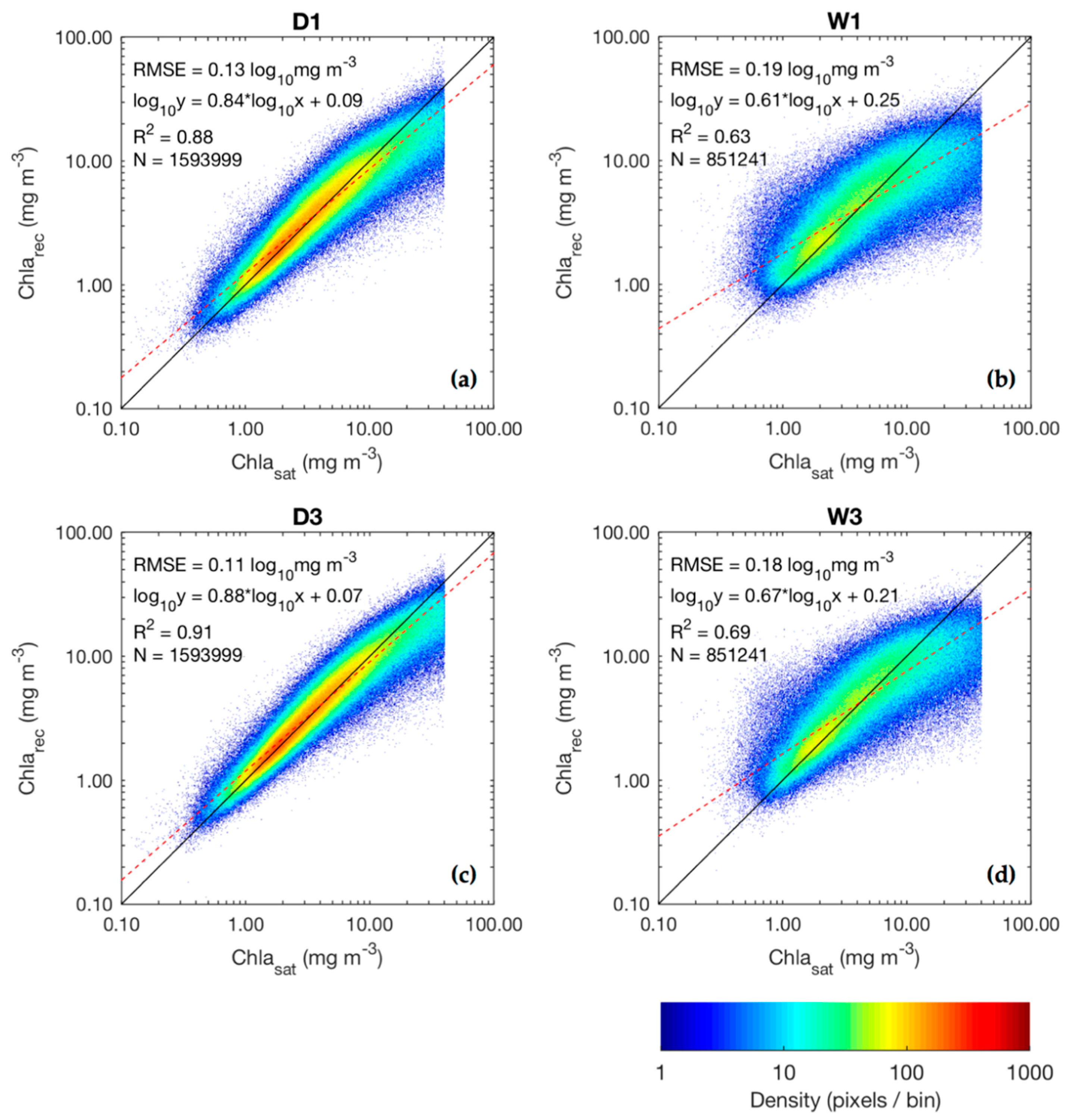
3.1. DINEOF Reconstruction Statistics

Higher performance was achieved for reconstructions of daily chla_sat over week composite (

Table 2. Variance of input chla_sat dataset captured during Data INterpolating Empirical Orthogonal Functions (DINEOF) processing, number of EOFs calculated, and corresponding RMSE_xval. RMSE_xval is also expressed in mg m⁻³.

	Explained Variance (%)	Calculated EOFs (#)	RMSExval (log10 mg m−3)	RMSExval (mg m−3)
D12014	96.05	11	0.22	1.65
D12015	96.33	9	0.21	1.61
D12016	95.08	9	0.20	1.58
D3	97.08	26	0.17	1.49
W12014	68.99	3	0.32	2.07
W12015	74.68	3	0.30	1.98
W12016	73.52	3	0.29	1.95
W3	76.88	8	0.27	1.87

), and when reconstructing datasets with more numerous input scenes (Table 1). Specifically, for daily reconstructions, the RMSE_xval ranged from 1.49 to 1.65 mg m⁻³, capturing 95.08% of the chla_sat variance with 9 EOFs for individual years (D1), and up to 97.08% with 26 EOFs for the multiyear dataset (D3). Week composite reconstructions demonstrated slightly higher RMSE_xval (1.87–2.07 mg m⁻³), with 68.99% of the chla_sat variance captured by three EOFs for yearly input data (W1) to 76.88% with 8 EOFs for multiyears (W3).

Similar to the global reconstruction results shown in Table 2, the statistical results of chla_rec when correlated with corresponding chla_sat pixels for all DINEOF implementations showed that daily reconstructions were improved relative to week composites, and the three-year input data time series produced slightly better results compared with annual counterparts (

Table 3. Annual relationship of chla_sat values to corresponding chla_rec pixels per time period for daily (a) and week composite (b) image time series.

(a)	R2	RMSE (log10 mg m−3)	RMSE (mg m−3)	Slope	Intercept	(b)	R2	RMSE (log10 mg m−3)	RMSE (mg m−3)	Slope	Intercept
D12014	0.88	0.13	1.35	0.85	0.08	W12014	0.61	0.20	1.58	0.59	0.25
D32014	0.91	0.11	1.29	0.88	0.07	W32014	0.70	0.19	1.55	0.67	0.20
D12015	0.87	0.13	1.35	0.83	0.10	W12015	0.62	0.19	1.55	0.59	0.27
D32015	0.91	0.11	1.29	0.87	0.07	W32015	0.67	0.18	1.51	0.64	0.23
D12016	0.87	0.13	1.35	0.84	0.09	W12016	0.65	0.19	1.55	0.63	0.23
D32016	0.92	0.11	1.29	0.89	0.07	W32016	0.71	0.18	1.51	0.69	0.20

, Figure 3). Specifically, D3 was superior to D1, showing the best results overall, producing the lowest RMSE_xval (0.17 log₁₀ mg m⁻³), lowest RMSE relative to chla_sat pixels (0.11 log₁₀ mg m⁻³ for all time resolutions), intercept nearest zero (0.07), highest R² (0.91), and slope closest to 1.00 (0.88) (Table 3a). Similar results were observed for W3 when compared with W1 reconstructions (Table 3b and Figure 3b,d), emphasizing the higher accuracy achievable for all pixels when time series with more input scenes were reconstructed. Further, the daily reconstructions exhibited the highest pixel density along the 1:1 line (Figure 3a,c), while week composite reconstructions demonstrated a greater spread of chla_sat and chla_rec values and poorer linear relationship to original chla_sat pixels (Figure 3b,d). It is evident that the distribution of chla_sat played a role in the reconstruction outcomes (Figure 3), as chla_rec were underestimated at higher concentrations (>20.00 mg m⁻³).

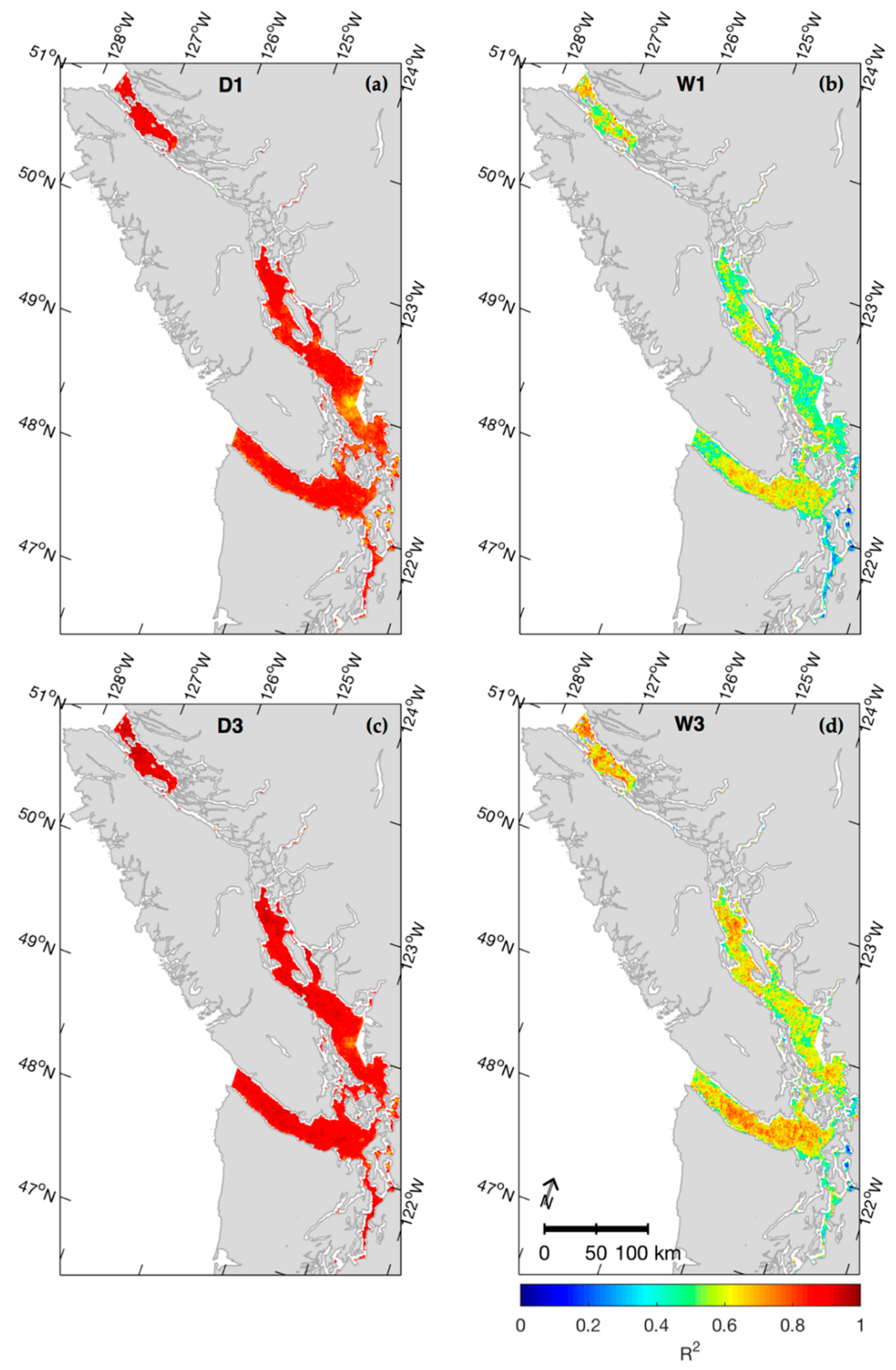
3.2. Spatiotemporal Accuracy of DINEOF Products

Spatially, the R² values calculated between chla_sat and chla_rec for each three-year pixel time series were relatively consistent throughout the study region and higher for daily reconstructions, while lower and more variable for week composite reconstructions (Figure 4). Specifically, the R² values of the D1 reconstruction for all pixels were predominantly high (>0.80), with the lowest values near the Fraser River discharge area (R² ~ 0.65–0.75, Figure 4a). This relationship was improved for D3 (R² predominantly > 0.90), with similar spatial pattern to D1, also reflecting the reduced relationship at the Fraser River plume area (R² ~ 0.70–0.85, Figure 4c). Conversely, week composite chla_rec showed much lower agreement to chla_sat for each pixel time series (R² < 0.80) (Figure 4b,d), exhibiting high spatial variation and very low values in the PS region (R² < 0.4). The highest R² occurred in the JFS, QCS, and northern SoG for W3 (R² ~ 0.70, Figure 4d). W1, similarly, exhibited the highest relationship (R² ~ 0.60) in JFS and QCS.

Temporally, differing reconstruction outcomes were evident for regions with missing chla_sat data. For example, a daily reconstruction from 28 February 2014 showed low chla_sat+rec for D3 (Figure 5c) at ~300 km along the thalweg, which is not present in the D1 chla_sat+rec image (Figure 5b). An example of a week composite image for the week of 2 April 2014 similarly demonstrated chla of higher magnitude, where chla_sat+rec is >25.0 mg m⁻³ at the entrance to the JFS for W3 (Figure 5f), while W1 remained between 5.0 and 20.0 mg m⁻³ (Figure 5e). In this example, W3 also reconstructed values below 1.0 mg m⁻³ in the SoG, while W1 more consistently showed chla from 2.5 to 5.0 mg m⁻³.

In a spatiotemporal example, chla_sat+rec along the Salish Sea thalweg for each time series are shown in Figure 6 and Figure 7. During spring of 2015 (late February through May), little spatial chla_sat data was available for both daily and week composite data in the Salish Sea north of ~250 km (Figure 6a and Figure 7a, respectively). D1 reconstructed an event of high chla_sat+rec lasting approximately 2 weeks during this period (Figure 6b), while the corresponding D3 time series demonstrated shorter duration and more localized high and low chla events (Figure 6c). For this time period, the week composite chla_sat+rec time series showed more similar results relative to one another (Figure 7) due to the constrained temporal dimension and lower missing data present for each scene, though W1 demonstrated higher- and lower-magnitude chla events during this time (Figure 7b). These examples demonstrate that, while statistical measures show high accuracy of chla_rec relative to chla_sat (Table 2 and Table 3), reconstructions where no spatial data existed previously are products of EOF calculations based on the input data alone, and can in turn impact further derived metrics such as bloom phenology.

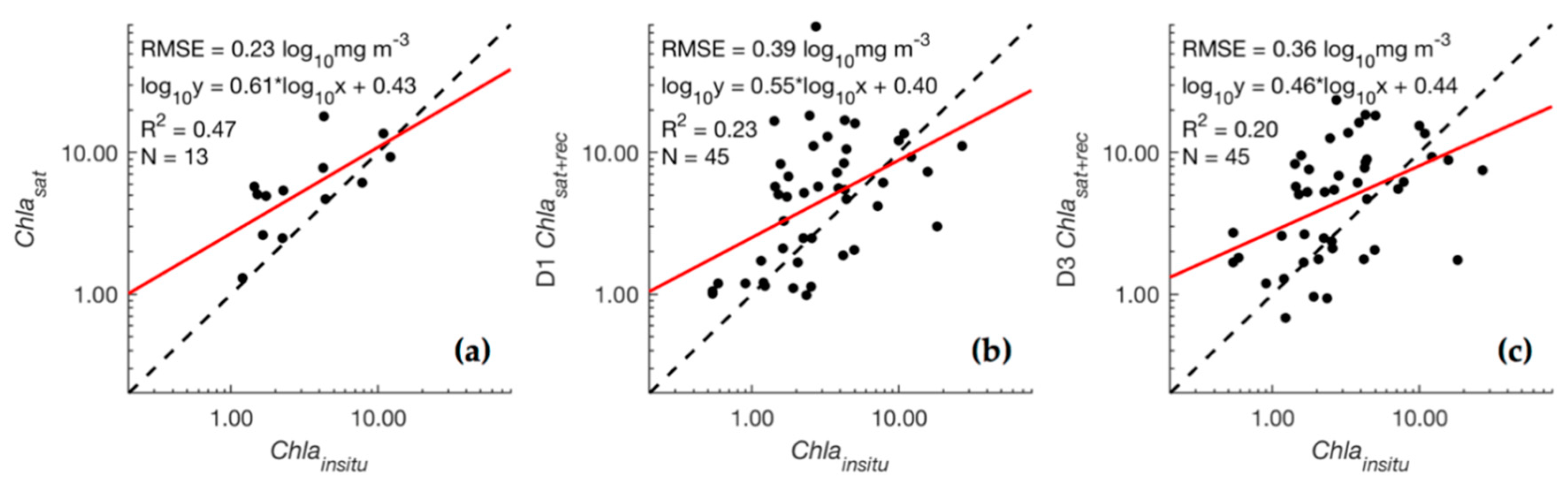
3.3. DINEOF-Reconstructed and In Situ Data

From a total of 374 chla_insitu samples acquired within ±3 h of daily satellite scenes, 15 and 45 were available for validating chla_sat and the DINEOF output chla_sat+rec, respectively. Note that while chla_sat pixels greater than 40.0 mg m⁻³ were removed from the input products (Section 2.2.1), reconstructed values (corresponding to <1% of the total pixels) were not filtered in this manner for the analysis, reflected in one of the D1 matchups. In general, both chla_sat and chla_sat+rec values were overestimated relative to the chla_insitu (Figure 8). chla_sat achieved the highest R² (0.47), slope nearest 1.0 (0.61), and lowest RMSE (0.23 log₁₀ mg m⁻³) relative to the chla_insitu. For the chla_sat+rec, the D1 matchups produced a higher R² (0.23) and slope closer to 1.00 (0.55) than the D3 chla_sat+rec, and achieved the poorest RMSE (0.39 log₁₀ mg m⁻³).

4. Discussion

The following sections provide a discussion of these results, emphasizing the role of the time scale of the input data on the DINEOF reconstruction accuracy considering prior studies from the Salish Sea and other dynamic regions of the world, and recommendations for using the DINEOF method.

4.1. Satellite-Derived versus DINEOF-Reconstructed chla

Overall, daily input time series produced more accurate chla reconstructions relative to week composite time series, and longer time periods produced better reconstructions. While many factors impact the outcomes of DINEOF for spatially reconstructing satellite datasets, including the input data characteristics, region, and processing parameters, our results can be explained mainly by the following:

• More spatial and temporal data allows physical processes to be more clearly resolved in time and space. As the degrees of freedom increase with longer time series, a higher number of EOFs can be calculated [8,47]. Consequently, finer-scale features (e.g., spatially localized events of shorter duration) and greater variance of the input dataset is captured, resulting in more accurate reconstructions. Additionally, differences in reconstruction accuracy year to year depended on the annual differences in input data. For example, 2016 demonstrated the highest R² and slope closest to 1.0 for the D3 (R² 0.92, slope 0.89), W1 (R² 0.65, slope 0.63), and W3 (R² 0.71, slope 0.69) reconstructions (Table 3), corresponding to the year with lowest percent missing data (71.65% and 37.82% for D1₂₀₁₆ and W1₂₀₁₆, respectively; Table 1).
• Poorly represented processes are more difficult to reconstruct. Week composite time series are more poorly reconstructed for this reason, as images often display spatially heterogeneous image features as a result of averaging the daily chla_sat scenes used in the binning process [2] (e.g., Figure 5d–f). EOF reconstruction methods usually produce spatially smoothed datasets, making spatial discontinuities more difficult to capture, particularly when only few EOF modes are calculated due to dataset size constraints. The long winter gaps present in D3 and W3 reconstructions also contribute to poorly constrained temporal EOFs.

As a result of these factors, longer time series (e.g., D3 over D1, and W3 over W1) produced the best DINEOF outcomes. D3, the input time series with most overall valid pixels and images, produced the best results in terms of reconstruction statistics and when assessed with chla_sat (Table 2 and Table 3). The shortest time series (W1), on the other hand, likely had insufficient images (Table 1) to capture enough information to reflect physical processes in so few EOFs [47]. For example, while 26 EOFs were calculated for D3, combining to capture 97.08% of the variance of the original input dataset, only three EOFs were calculated for each W1 year, capturing from 68.99 to 74.68% of the input dataset variance. However, using DINEOF with so few input datapoints (W1 had between 34 and 35 scenes as input) is generally not recommended due to the low number of degrees of freedom and the decreased ability to capture physical trends [10]. Ref. [12] found that with at least 35 input scenes, a stable RMSE_xval was achieved when reconstructing SST data; a similar test performed with our dataset showed equal results (not shown).

The improved DINEOF results of daily input data were evident when examining the temporal R² between chla_sat and chla_rec throughout the study region (Figure 4). For D3 and D1 (Figure 4a,c), the R² was >0.80 for most of the Salish Sea. However, a region of lower reconstruction effectiveness (R² ~ 0.75 for D3, ~0.60 for D1) occurred nearest the Fraser River plume. Two factors may play a role in the lower reconstruction effectiveness here. Fraser plume waters are documented to negatively impact retrievals of OC3M chla [39], which may have resulted in reduced temporal variability of chla, with consequences on the daily DINEOF reconstructions. Additionally, DINEOF reconstructions have been demonstrated to perform better in regions of high variability, as opposed to in more homogeneous waters [2,52]. Greater temporal homogeneity of chla in the Fraser River plume is evident in Figure 6a–c and Figure 7a–c, (located at ~250 km distance along the Salish Sea thalweg). Figure 9 further shows the poorer performance of chla reconstruction of Fraser plume waters compared with JFS for the time series. The relationship between D3 chla_sat and chla_rec pixels from near the Fraser plume shows more homogeneous chla concentrations, ranging between ~3.00 and 13.00 mg m⁻³, in contrast to the JFS, where concentrations had a larger range (from 0.40 to 40.00 mg m⁻³) and an improved linear relationship was observed. In our case, lower R² may have been a result of less variable chla_sat over the time series nearest the Fraser River plume relative to other regions of the Salish Sea. The corresponding W3 chla_sat and chla_rec data for the same regions also shows a poorer relationship for Fraser River plume waters compared with JFS (Figure 9c,d).

The relatively poorer performance of week composite DINEOF reconstructions may be contrary to expected, considering the much higher spatial coverage per image when compared with daily images. The poor week composite performance is a result of the greatly reduced temporal dimension (Table 1), combined with the higher spatial heterogeneity of chla (Figure 5c–e and Figure 7). However, in studies for longer time series (e.g., [16]), week composite data may be preferable where the temporal and spatial scale of features to be resolved are not negatively impacted by the lower temporal coverage. As shown in Figure 7 and Figure A1, the spatiotemporal time series of W1 and W3 were consistent relative to each other, as compared with the D1 and D3 chla_sat+rec time series, which demonstrated greater differences in image median and standard deviation values compared with chla_sat. This is in part due to the higher spatial coverage of chla_sat present in the week composite scenes, which reduces the impact of reconstructed values on these image statistics. Further research should include comparison of reconstructed week composite images based on longer time series, or relative to week composites made from reconstructed daily images as used in some studies (e.g., [53]).

Among the daily reconstruction results, annual (D1) and three-year reconstructions (D3) produced very similar correlations (Table 3a, Figure 3a,b) and RMSE_xval values (Table 2) for chla_sat and chla_rec, and high per-pixel temporal R² (Figure 4). D1 showed a slightly improved R² relative to D3 chla_insitu matchups (0.23 over 0.21), slope closer to 1.00 (0.55 over 0.46), and lower intercept (0.40 log₁₀ mg m⁻³ over 0.44 log₁₀ mg m⁻³). D1 had fewer EOFs calculated (2014: 11, 2015: 9, 2016: 9) than the D3 reconstruction (26), yet nearly equivalent variance of the chla_sat datasets was captured (Table 2) in faster processing time (~4× faster than D3). Besides the improved processing time, more EOFs are not always better, as separability of the EOF modes declines as more are calculated, and there is a higher likelihood of representing patterns that may not exist in reality [54]. Further, limiting the distribution of input chla_sat concentrations by year eliminated long winter gaps, which led to better-constrained EOFs. Figure A1 demonstrates the effect of long winter gaps in this time series on the per-scene median and standard deviation. D3 exhibited erroneously high chla_sat+rec median and standard deviation in some images (e.g., 16.00 ± 12.00 mg m⁻³ in November 2015) compared with D1 (3.00 ± 3.50 mg m⁻³ at the corresponding time). Given these advantages, D1 is a preferable alternative to multiyear input data for datasets with long winter gaps and dynamic spatiotemporal phytoplankton phenology.

While this study provides new insights on the effects of the data form and length of the input time series on DINEOF outcomes, other factors that impact reconstruction accuracy include the length of temporal data gaps (i.e., consecutive missing days or weeks), study area extent, and parameters used to reconstruct the dataset (e.g., temporal covariance filter length and the values of input pixels [10]). For example, the order of images in a time series should not impact the reconstruction results [10,55]. However, as illustrated here, long gaps between scenes, such as periods of missing data during winter months, can lead to calculation of irrelevant EOFs and unrealistically high/low chla (Figure A1), similar to results by [47]. The missing data of this study (Table 1) is comparable relative to other DINEOF studies (e.g., 75.2% missing daily data in [12], 63.3–75.5% in [14]; or, 39.4% missing for week composite time series in [16]) or even lower (e.g., 88.0% missing data in [22], or 86.0% missing in [56]). Improved results may be achieved in the future by using a longer time series to better constrain the EOFs near long gaps, or by using a longer temporal covariance matrix filter [47]. Additionally, the quality of input data is an important consideration for using DINEOF and is affected by the inherited uncertainties of the chla_sat [57]. In this study, quality control prior to DINEOF processing included standard ocean color flags, a reduced straylight filter (3 × 3), removal of chla_sat pixels exceeding 40.00 mg m⁻³ (Section 2.2.1), and removal of scenes and pixels with less than 2% ocean coverage (Section 2.3). However, outlier or erroneous pixels, such as at undetected cloud edges [40], may have been introduced through the straylight flag reduction, or in scenes with low spatial coverage. Additionally, the removal of pixels exceeding 40.00 mg m⁻³, while consistent with other remote sensing chla studies of the region [35,58], resulted in a distinctive distribution of input data (Figure 3). This led to a reduction of the global input dataset mean, and, as a result, chla_rec concentrations above ~20.0 mg m⁻³ were underestimated as data was reconstructed following a normal distribution of the input dataset anomaly (Section 2.3.1). Beyond the quality control methods employed here, other techniques used with DINEOF including limiting the number of scenes per month for temporal consistency [23], stricter spatial coverage requirements [55], and applying various methods for statistical detection and removal of outlier pixels [2,18,59] should be considered in further use.

4.2. Accuracy of chla_sat and Reconstructed Products

The evaluation of the satellite- and DINEOF-derived products used in this study relative to available in situ matchups showed that the original chla_sat achieved a better relationship to in situ matchups than did reconstructed chla_sat+rec, though far fewer matchup datapoints were available for the former. The original chla_sat matchups and DINEOF-reconstructed chla_sat+rec produced RMSE values of 2.45 mg m⁻³ (R² 0.23) and 2.29 mg m⁻³ (R² 0.20) for D1 and D3, respectively (Figure 8). The chla_sat matchup statistics (RMSE of 1.70 mg m⁻³ and R² 0.47) are within the global OC3M RMSE for MODISA chla (2.10 mg m⁻³) [36]. While the DINEOF-reconstructed chla_sat+rec RMSEs are slightly higher, these values are of similar magnitude to those found by [60], who showed a DINEOF-reconstructed SeaWiFs chla RMSE of 2.50 mg m⁻³ for the Yangtze River estuary, and similar to MODISA-derived chla from previous studies in the Salish Sea for in situ extracted chla (RMSE 2.14 mg m⁻³ and R² 0.54) [35] and ferry-measured in situ fluorimetric measurements (RMSE 2.63 mg m⁻³ and R² 0.72) [38].

Although the resulting accuracy of the reconstructions (e.g., RMSE_xval, RMSE of chla_rec to chla_sat), is within published satellite-derived chla concentration measures, the reconstructed chla shows both over- and underestimation across the range of concentrations (Figure 8). This is likely largely due to spatial biases of the available in situ data, combined with inherent inaccuracies of standard bio-optical algorithms for MODISA in complex coastal environments [50]. The matchups used here were mostly from waters under the influence of the Fraser River plume, where OC3M chla estimates are negatively impacted [35,38,39]. High concentrations of suspended matter and dissolved organic matter, in addition to tidal activity, wind, and river discharge, make this region dynamic and optically complex [34], adding difficulties to accurate satellite retrievals and time/space matchups [35,38] and, consequently, to the DINEOF reconstruction. The low number of in situ matchups is often a limitation for validation of satellite data [35], including in the evaluation of DINEOF-reconstructed datasets.

5. Conclusions

Derivation of phytoplankton phenology from satellite sensors is challenged by missing data [15]. In this study, the DINEOF method was applied to Salish Sea MODISA-derived chla products spanning a three-year time period to investigate the accuracy of the derived products according to dataset study period, yearly versus multiyear, and forms of input data, daily versus week composite.

Although other studies use DINEOF for reconstructing chla for further analyses (e.g., [15,61]), the current study demonstrated that considering the temporal characteristics of an input dataset is an important factor in the effectiveness of the chla reconstruction accuracy. Specifically, the greater spatial coverage of the week composite dataset was not an advantage for chla reconstruction relative to the corresponding daily image time series for a given study period. The daily time series will always contain more scenes and overall available data points, which allows for the calculation of a higher number of EOFs, thus capturing higher variance of the original dataset. The greater spatial heterogeneity of the week composite imagery combined with the low number of scenes for this study period led to inferior results. For daily input data, the implementations were faster to process, with the advantage of annually constraining the EOF basis (distribution of chla). When utilizing matchup data to validate the daily input chla_sat and reconstructed chla_sat+rec imagery, measures of error were comparable to those in other studies where chla was retrieved with the OC3M method for the study region, and with global datasets. In addition, while chla remains difficult to reconstruct and further quality control improvements are necessary for this dataset, the global accuracies of the chla_rec compared to the original chla_sat data were within the range of other similar studies and remotely sensed chla errors.

While all interpolation methods have caveats, the DINEOF method exhibits some major advantages compared with many others [8], including the minimization of error from iterative processing, parameter-free processing, and speed. The findings and recommendations raised in this study can assist further DINEOF studies by demonstrating the dependence of results on the input data characteristics. Importantly, the accuracy requirements of a given study and scale of physical processes should guide selection of the appropriate form and period of input data. Further, studies should consider quality control improvements and gap-filling of a multisensor time series to utilize the greatest amount of chla for the satellite data record.

DINEOF is a robust tool enabling a multitude of further applications for satellite datasets, such as construction of spatially continuous fields for biogeochemical or ecosystem modelling [62], smoothing and noise reduction, and analyzing phenology and correlations between geophysical variables [61]. For the west coast of Canada, the results of this study facilitate production of chla datasets more effective for studying long-term trends and addressing broader ecological questions, including assisting with fisheries management.

References

1. Mélin, F.; Vantrepotte, V.; Chuprin, A.; Grant, M.; Jackson, T.; Sathyendranath, S. Assessing the Fitness-for-Purpose of Satellite Multi-Mission Ocean Color Climate Data Records: A Protocol Applied to OC-CCI Chlorophyll-a Data. Remote Sens. Environ. 2017. [Google Scholar] [CrossRef] [PubMed]
2. Sirjacobs, D.; Alvera-Azcárate, A.; Barth, A.; Lacroix, G.; Park, Y.; Nechad, B.; Ruddick, K.; Beckers, J.M. Cloud Filling of Ocean Colour and Sea Surface Temperature Remote Sensing Products over the Southern North Sea by the Data Interpolating Empirical Orthogonal Functions Methodology. J. Sea Res. 2011, 65, 114–130. [Google Scholar] [CrossRef]
3. IOCCG. IOCCG Report Number 4: Guide to the Creation and Use of Ocean-Colour, Level-3, Binned Data Products; Antoine, D., Ed.; IOCCG: Dartmouth, DC, Canada, 2004. [Google Scholar]
4. Kahru, M.; Kudela, R.M.; Manzano-Sarabia, M.; Greg Mitchell, B. Trends in the Surface Chlorophyll of the California Current: Merging Data from Multiple Ocean Color Satellites. Deep. Res. Part II Top. Stud. Oceanogr. 2012, 77–80, 89–98. [Google Scholar] [CrossRef]
5. Bennett, A.F. Inverse Modeling of the Ocean and Atmosphere, 1st ed.; Cambridge University Press: Cambridge, UK, 2002. [Google Scholar]
6. Casey, B.; Arnone, R.; Flynn, P. Simple and Efficient Technique for Spatial/Temporal Composite Imagery. Proc. SPIE 2007, 6680, 1–8. [Google Scholar] [CrossRef]
7. Müller, D. Estimation of Algae Concentration in Cloud Covered Scenes Using Geostatistical Methods. In Proceedings of the Envisat Symposium 2007, Montreux, Switzerland, 23–27 April 2007. [Google Scholar]
8. Taylor, M.H.; Losch, M.; Wenzel, M.; Schröter, J.; Taylor, M.H.; Losch, M.; Wenzel, M.; Schröter, J. On the Sensitivity of Field Reconstruction and Prediction Using Empirical Orthogonal Functions Derived from Gappy Data. J. Clim. 2013, 26, 9194–9205. [Google Scholar] [CrossRef] [Green Version]
9. Beckers, J.M.; Rixen, M. EOF Calculations and Data Filling from Incomplete Oceanographic Datasets. J. Atmos. Ocean. Technol. 2003, 20, 1839–1856. [Google Scholar] [CrossRef]
10. Alvera-Azcárate, A.; Barth, A.; Rixen, M.; Beckers, J.M. Reconstruction of Incomplete Oceanographic Data Sets Using Empirical Orthogonal Functions: Application to the Adriatic Sea Surface Temperature. Ocean Model. 2005, 9, 325–346. [Google Scholar] [CrossRef] [Green Version]
11. Beckers, J.M.; Barth, A.; Alvera-Azcárate, A. DINEOF Reconstruction of Clouded Images Including Error Maps. Application to the Sea-Surface Temperature around Corsican Island. Ocean Sci. Discuss. 2006, 2, 183–199. [Google Scholar] [CrossRef]
12. Ganzedo, U.; Alvera-Azcárate, A.; Esnaola, G.; Ezcurra, A.; Sáenz, J. Reconstruction of Sea Surface Temperature by Means of DINEOF: A Case Study during the Fishing Season in the Bay of Biscay. Int. J. Remote Sens. 2011, 32, 933–950. [Google Scholar] [CrossRef]
13. Li, Y.; He, R. Spatial and Temporal Variability of SST and Ocean Color in the Gulf of Maine Based on Cloud-Free SST and Chlorophyll Reconstructions in 2003–2012. Remote Sens. Environ. 2014, 144, 98–108. [Google Scholar] [CrossRef]
14. Alvera-Azcárate, A.; Barth, A.; Parard, G.; Beckers, J.M. Analysis of SMOS Sea Surface Salinity Data Using DINEOF. Remote Sens. Environ. 2016, 180, 137–145. [Google Scholar] [CrossRef]
15. Corredor-Acosta, A.; Morales, C.E.; Hormazabal, S.; Andrade, I.; Correa-Ramirez, M.A. Phytoplankton Phenology in the Coastal Upwelling Region off Central-Southern Chile (35S–38S): Time-Space Variability, Coupling to Environmental Factors, and Sources of Uncertainty in the Estimates. J. Geophys. Res. C Ocean. 2015, 120, 813–831. [Google Scholar] [CrossRef]
16. Waite, J.N.; Mueter, F.J. Spatial and Temporal Variability of Chlorophyll-a Concentrations in the Coastal Gulf of Alaska, 1998–2011, Using Cloud-Free Reconstructions of SeaWiFS and MODIS-Aqua Data. Prog. Oceanogr. 2013, 116, 179–192. [Google Scholar] [CrossRef]
17. Liu, X.; Wang, M. Gap Filling of Missing Data for VIIRS Global Ocean Color Products Using the DINEOF Method. IEEE Trans. Geosci. Remote Sens. 2018, 56, 4464–4476. [Google Scholar] [CrossRef]
18. Alvera-Azcárate, A.; Vanhellemont, Q.; Ruddick, K.; Barth, A.; Beckers, J.M. Analysis of High Frequency Geostationary Ocean Colour Data Using DINEOF. Estuar. Coast. Shelf Sci. 2015, 159, 28–36. [Google Scholar] [CrossRef]
19. Nechad, B.; Alvera-Azcárate, A.; Ruddick, K.; Greenwood, N. Reconstruction of MODIS Total Suspended Matter Time Series Maps by DINEOF and Validation with Autonomous Platform Data. Ocean Dyn. 2011, 61, 1205–1214. [Google Scholar] [CrossRef]
20. Shropshire, T.; Li, Y.; He, R. Storm Impact on Sea Surface Temperature and Chlorophyll a in the Gulf of Mexico and Sargasso Sea Based on Daily Cloud-Free Satellite Data Reconstructions. Geophys. Res. Lett. 2016, 43, 12199–12207. [Google Scholar] [CrossRef]
21. Miles, T.N.; He, R.; Li, M. Characterizing the South Atlantic Bight Seasonal Variability and Cold-Water Event in 2003 Using a Daily Cloud-Free SST and Chlorophyll Analysis. Geophys. Res. Lett. 2009, 36, 1–6. [Google Scholar] [CrossRef]
22. Huynh, H.-N.T.; Alvera-Azcárate, A.; Barth, A.; Beckers, J.-M. Reconstruction and Analysis of Long-Term Satellite-Derived Sea Surface Temperature for the South China Sea. J. Oceanogr. 2016, 72, 707–726. [Google Scholar] [CrossRef]
23. Mauri, E.; Poulain, P.M.; Južnič-Zonta, Ž. MODIS Chlorophyll Variability in the Northern Adriatic Sea and Relationship with Forcing Parameters. J. Geophys. Res. Ocean. 2007, 112, 1–14. [Google Scholar] [CrossRef]
24. Johannessen, S.C.; Macdonald, R.W.; Paton, D.W. A Sediment and Organic Carbon Budget for the Greater Strait of Georgia. Estuar. Coast. Shelf Sci. 2003, 56, 845–860. [Google Scholar] [CrossRef]
25. Masson, D. Seasonal Water Mass Analysis for the Straits of Juan de Fuca and Georgia. Atmosphere 2006, 44, 1–15. [Google Scholar] [CrossRef]
26. Porter, A.D.; Rechisky, E.L.; Winchell, P.; Welch, D.W. The Use of Telemetry to Investigate Residence Time and Survival of Fraser River Chinook Salmon in the Strait of Georgia, 2016: Final Report to the Pacific Salmon Foundation and the Salish Sea Marine Survival Project; Kintama Research Services: Nanaimo, BC, Canada, 2016. [Google Scholar]
27. Yin, K.; Goldblatt, R.H.; Harrison, P.J.; St. John, M.A.; Clifford, P.J.; Beamish, R.J. Importance of Wind and River Discharge in Influencing Nutrient Dynamics and Phytoplankton Production in Summer in the Central Strait of Georgia. Mar. Ecol. Prog. Ser. 1997, 161, 173–183. [Google Scholar] [CrossRef] [Green Version]
28. Collins, A.K.; Allen, S.E.; Pawlowicz, R. The Role of Wind in Determining the Timing of the Spring Bloom in the Strait of Georgia. Can. J. Fish. Aquat. Sci. 2009, 66, 1597–1616. [Google Scholar] [CrossRef]
29. Li, M.; Gargett, A.; Denman, K. What Determines Seasonal and Interannual Variability of Phytoplankton and Zooplankton in Strongly Estuarine Systems? Application to the Semi-Enclosed Estuary of Strait of Georgia and Juan de Fuca Strait. Estuar. Coast. Shelf Sci. 2000, 50, 467–488. [Google Scholar] [CrossRef]
30. Allen, S.E.; Wolfe, M.A. Hindcast of the Timing of the Spring Phytoplankton Bloom in the Strait of Georgia, 1968–2010. Prog. Oceanogr. 2013, 115, 6–13. [Google Scholar] [CrossRef]
31. Perry, R.I. Plankton Blooms of the British Columbia Northern Shelf: Seasonal Distributions and Mechanisms Influencing Their Formation; University of British Columbia: Vancouver, BC, Canada, 1984. [Google Scholar]
32. Mackas, D.L.; Louttit, G.C.; Austin, M.J. Spatial Distribution of Zooplankton and Phytoplankton in British Columbian Coastal Waters. Can. J. Fish. Aquat. Sci. 1980, 37, 1476–1487. [Google Scholar] [CrossRef]
33. Phillips, S.R.; Costa, M. Spatial-Temporal Bio-Optical Classification of Dynamic Semi-Estuarine Waters in Western North America. Estuar. Coast. Shelf Sci. 2017, 199, 35–48. [Google Scholar] [CrossRef]
34. Loos, E.A.; Costa, M. Inherent Optical Properties and Optical Mass Classification of the Waters of the Strait of Georgia, British Columbia, Canada. Prog. Oceanogr. 2010, 87, 144–156. [Google Scholar] [CrossRef]
35. Carswell, T.; Costa, M.; Young, E.; Komick, N.; Gower, J.; Sweeting, R. Evaluation of MODIS-Aqua Atmospheric Correction and Chlorophyll Products of Western North American Coastal Waters Based on 13 Years of Data. Remote Sens. 2017, 9, 1063. [Google Scholar] [CrossRef]
36. NASA Ocean Color. Available online: https://oceancolor.gsfc.nasa.gov/ (accessed on 1 September 2015).
37. NASA SeaDAS. Available online: https://seadas.gsfc.nasa.gov/ (accessed on 1 September 2015).
38. Komick, N.M. Remote Sensing Chlorophyll-a in the Strait of Georgia; University of Victoria: Victoria, BC, Canada, 2007. [Google Scholar]
39. Komick, N.M.; Costa, M.P.F.; Gower, J. Bio-Optical Algorithm Evaluation for MODIS for Western Canada Coastal Waters: An Exploratory Approach Using in Situ Reflectance. Remote Sens. Environ. 2009, 113, 794–804. [Google Scholar] [CrossRef]
40. Meister, G.; Zong, Y.; McClain, C.R. Derivation of the MODIS Aqua Point-Spread Function for Ocean Color Bands. Proc. SPIE 2008, 7081, 70811F-1–70811F-12. [Google Scholar] [CrossRef]
41. Fisheries and Oceans Canada, Pacific Region, OSD. Institute of Ocean Sciences Data Archive. Available online: http://www.pac.dfo-mpo.gc.ca/science/oceans/data-donnees/search-recherche/profiles-eng.asp (accessed on 28 August 2017).
42. Barwell-Clarke, J.; Whitney, F. Canadian Technical Report of Hydrography and Ocean Sciences No. 182, Institute of Ocean Sciences Nutrient Methods and Analysis; Institute of Ocean Sciences: Sidney, BC, Canada, 1996. [Google Scholar]
43. Holm-Hansen, O.; Lorenzen, C.J.; Holmes, R.W.; Strickland, J.D.H. Fluorometric Determination of Chlorophyll. J. Cons. Perm. Int. Explor. Mer. 1965, 30, 3–15. [Google Scholar] [CrossRef] [Green Version]
44. Alvera-Azcárate, A.; Barth, A.; Sirjacobs, D.; Lenartz, F.; Beckers, J.-M. Data Interpolating Empirical Orthogonal Functions (DINEOF): A Tool for Geophysical Data Analyses. Medit. Mar. Sci. Spec. Issue 2011, 5–11. [Google Scholar] [CrossRef]
45. DINEOF—GHER. Available online: http://modb.oce.ulg.ac.be/mediawiki/index.php/DINEOF (accessed on 1 October 2016).
46. Campbell, J.W. The Lognormal Distribution as a Model for Bio-Optical Variability in the Se. J. Geophys. Res. Oceans 1995, 100, 237–254. [Google Scholar] [CrossRef]
47. Alvera-Azcárate, A.; Barth, A.; Sirjacobs, D.; Beckers, J.-M. Enhancing Temporal Correlations in EOF Expansions for the Reconstruction of Missing Data Using DINEOF. Ocean Sci. Discuss. 2009, 6, 1547–1568. [Google Scholar] [CrossRef]
48. Wilks, D.S. Statistical Methods in the Atmospheric Sciences, 2nd ed.; Academic Press: London, UK, 2006. [Google Scholar]
49. Brewin, R.J.W.; Mélin, F.; Sathyendranath, S.; Steinmetz, F.; Chuprin, A.; Grant, M. On the Temporal Consistency of Chlorophyll Products Derived from Three Ocean-Colour Sensors. ISPRS J. Photogramm. Remote Sens. 2014, 97, 171–184. [Google Scholar] [CrossRef]
50. Bailey, S.W.; Werdell, P.J. A Multi-Sensor Approach for the on-Orbit Validation of Ocean Color Satellite Data Products. Remote Sens. Environ. 2006, 102, 12–23. [Google Scholar] [CrossRef]
51. Werdell, P.J.; Bailey, S.W.; Franz, B.A.; Harding, L.W.; Feldman, G.C.; McClain, C.R. Regional and Seasonal Variability of Chlorophyll-a in Chesapeake Bay as Observed by SeaWiFS and MODIS-Aqua. Remote Sens. Environ. 2009, 113, 1319–1330. [Google Scholar] [CrossRef]
52. Wang, Y.; Liu, D. Reconstruction of Satellite Chlorophyll-a Data Using a Modified DINEOF Method: A Case Study in the Bohai and Yellow Seas, China. Int. J. Remote Sens. 2014, 35, 204–217. [Google Scholar] [CrossRef]
53. Marchese, C.; Albouy, C.; Tremblay, J.-É.; Dumont, D.; D’Ortenzio, F.; Vissault, S.; Bélanger, S. Changes in Phytoplankton Bloom Phenology over the North Water (NOW) Polynya: A Response to Changing Environmental Conditions. Polar Biol. 2017, 40, 1721–1737. [Google Scholar] [CrossRef]
54. Strang, G. Linear Algebra and Its Applications, 3rd ed.; Harcourt-Brace-Jovanovich: San Diego, CA, USA, 1988. [Google Scholar]
55. Mauri, E.; Poulain, P.-M.; Notarstefano, G. Spatial and Temporal Variability of the Sea Surface Temperature in the Gulf of Trieste between January 2000 and December 2006. J. Geophys. Res. 2008, 113. [Google Scholar] [CrossRef]
56. Ping, B.; Su, F.; Meng, Y. An Improved DINEOF Algorithm for Filling Missing Values in Spatio-Temporal Sea Surface Temperature Data. PLoS ONE 2016, 11. [Google Scholar] [CrossRef] [PubMed]
57. Land, P.; Bailey, T.; Taberner, M.; Pardo, S.; Sathyendranath, S.; Nejabati Zenouz, K.; Brammall, V.; Shutler, J.; Quartly, G. A Statistical Modeling Framework for Characterising Uncertainty in Large Datasets: Application to Ocean Colour. Remote Sens. 2018, 10, 695. [Google Scholar] [CrossRef]
58. Jackson, J.M.; Thomson, R.E.; Brown, L.N.; Willis, P.G.; Borstad, G.A. Satellite Chlorophyll off the British Columbia Coast, 1997–2010. J. Geophys. Res. Ocean. 2015, 120, 4709–4728. [Google Scholar] [CrossRef]
59. Alvera-Azcárate, A.; Sirjacobs, D.; Barth, A.; Beckers, J.M. Outlier Detection in Satellite Data Using Spatial Coherence. Remote Sens. Environ. 2012, 119, 84–91. [Google Scholar] [CrossRef]
60. Wang, Y.; Jiang, H.; Jin, J.; Zhang, X.; Lu, X.; Wang, Y. Spatial-Temporal Variations of Chlorophyll-a in the Adjacent Sea Area of the Yangtze River Estuary Influenced by Yangtze River Discharge. Int. J. Environ. Res. Public Health 2015, 12, 5420–5438. [Google Scholar] [CrossRef] [PubMed] [Green Version]
61. McGinty, N.; Guðmundsson, K.; Ágústsdóttir, K.; Marteinsdóttir, G. Environmental and Climactic Effects of Chlorophyll-a Variability around Iceland Using Reconstructed Satellite Data Fields. J. Mar. Syst. 2016, 163, 31–42. [Google Scholar] [CrossRef]
62. Gregg, W.W. Assimilation of SeaWiFS Ocean Chlorophyll Data into a Three-Dimensional Global Ocean Model. J. Mar. Syst. 2008, 69, 205–225. [Google Scholar] [CrossRef]
Figure 1. The Salish Sea, oceanic and geographic features, and population centers. The region includes the Juan de Fuca Strait (JFS), Strait of Georgia (SoG), Puget Sound (PS), and Queen Charlotte Strait (QCS). QCS is included in this study considering its use in salmon migration research [26]. Locations of in situ chla matchups (Section 2.4.2) are indicated by blue (DINEOF-reconstructed chla) and blue-ringed circles (satellite and DINEOF-reconstructed chla).
Remotesensing 10 01449 g001
Figure 2. Temporal coverage displayed as (a) number of images per month and (b) percent spatial coverage of the study region per month. Presence of a given pixel is shown for (c) the daily time series and (d) week composite.
Remotesensing 10 01449 g002
Figure 3. D1 (a), W1 (b), D3 (c), and W3 (d) linear correlation results. The 40.00 mg m−3 threshold (Section 2.2.1) is evident as a cutoff feature in all plots.
Remotesensing 10 01449 g003
Figure 4. Per-pixel R2 of DINEOF results for D1 (a), W1 (b), D3 (c), and W3 (d).
Remotesensing 10 01449 g004
Figure 5. Daily reconstruction of February 28, 2014, shown as the original chlasat (a), D1 chlasat+rec (b), and D3 chlasat+rec (c); similarly, the week composite chlasat (d), W1 chlasat+rec (e), and W3 chlasat+rec (f). Salish Sea thalweg is shown in (a), with a gap excluding the region of no data in Johnstone Strait.
Remotesensing 10 01449 g005
Figure 6. Daily image time series shown as Hovmöller plot along Salish Sea thalweg (y axis, shown in Figure 5a), contrasting chlasat (a), D1 chlasat+rec (b), and D3 chlasat+rec (c) for 2014–2016. The dashed line represents a spatial gap in Johnstone Strait due to the inability of MODISA to resolve data in the narrow passages.
Remotesensing 10 01449 g006
Figure 7. Week composite time series extracted along the Salish Sea thalweg (y axis, Figure 5a) for chlasat (a), W1 chlasat+rec (b), and W3 chlasat+rec (c) for 2014–2016.
Remotesensing 10 01449 g007
Figure 8. Statistical results for chlainsitu between chlasat (a), D1 chlasat+rec (b), and D3 chlasat+rec (c). All p-values are <0.05.
Remotesensing 10 01449 g008
Figure 9. Relationship between original and reconstructed pixel time series for a D3 example pixel located in the Fraser River plume (a) and in central JFS (b), and for the W3 reconstruction in (c,d), respectively.
Remotesensing 10 01449 g009