Evaluation of Semi-Analytical Algorithms to Retrieve Particulate and Dissolved Absorption Coefficients in Gulf of California Optically Complex Waters

 ,
,  ,
,  ,
,  and
and
Abstract
1. Introduction
2. Materials and Methods
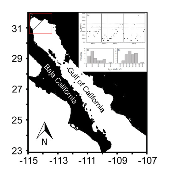
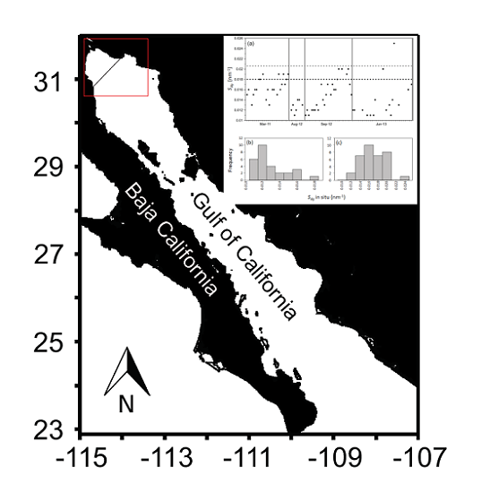
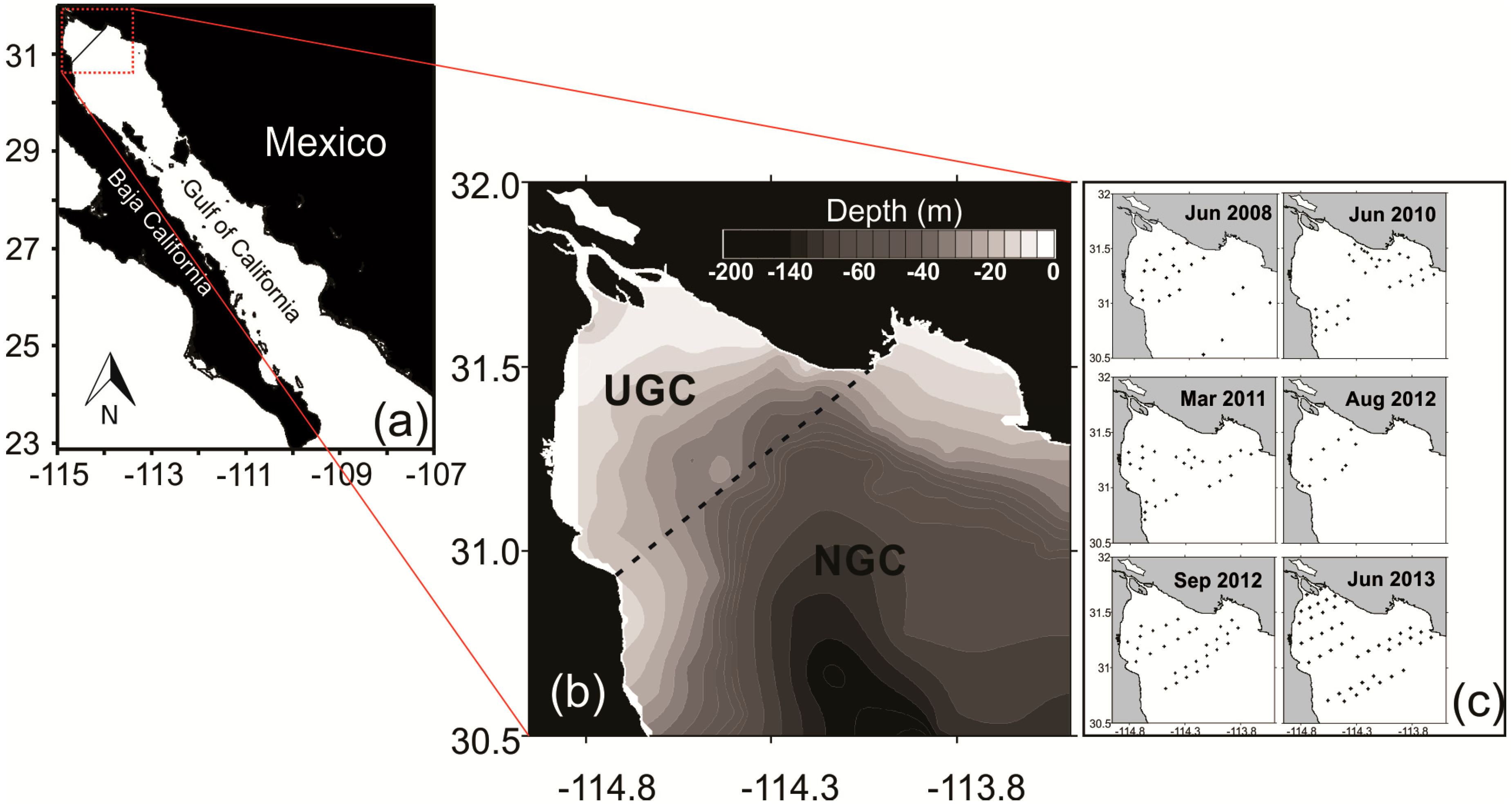
2.1. Study Area
2.2. In Situ Data
2.3. Satellite Data
2.4. Semi-Analytical Algorithms
2.5. Algorithm Evaluation Methodology
Pearson’s Correlation Coefficient (rp)
Root Mean Square Error (RMSE)
Bias
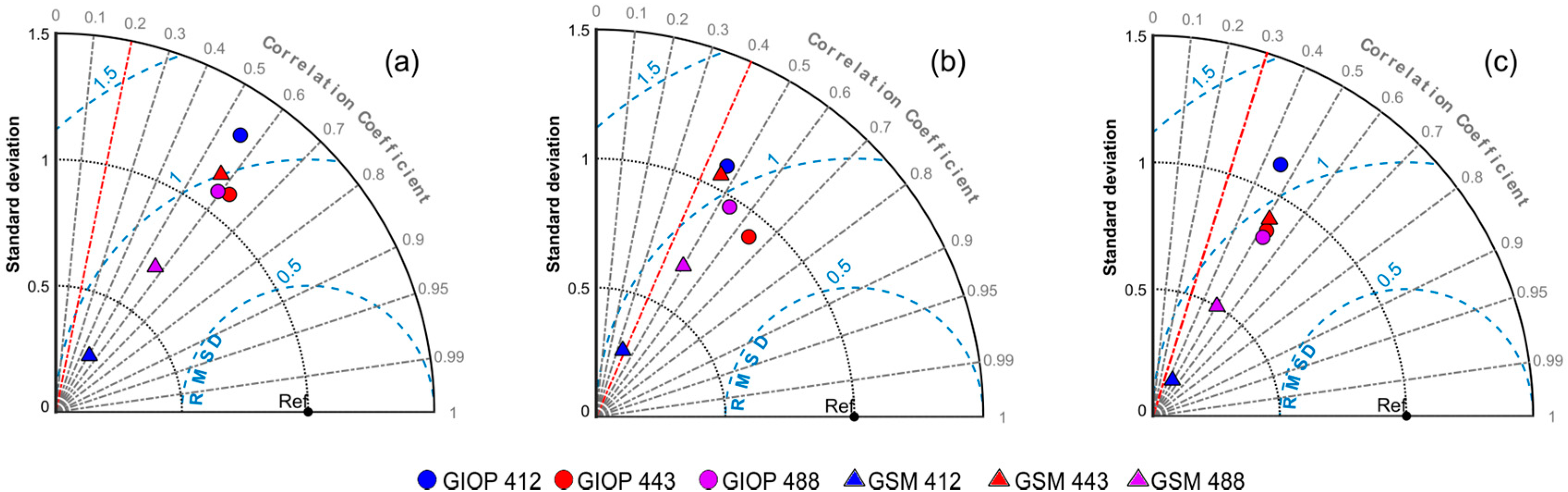
Taylor Diagram
3. Results and Discussion
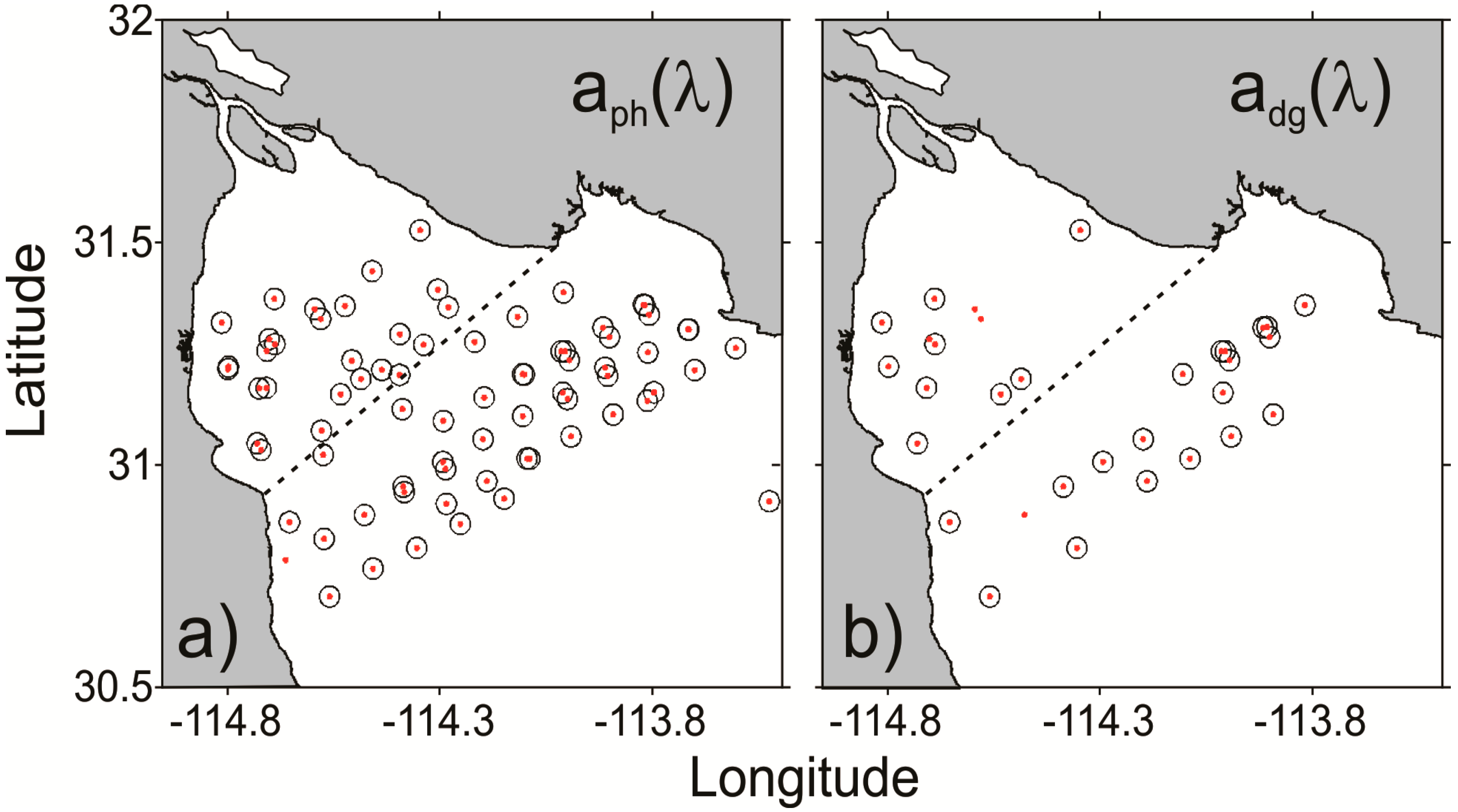
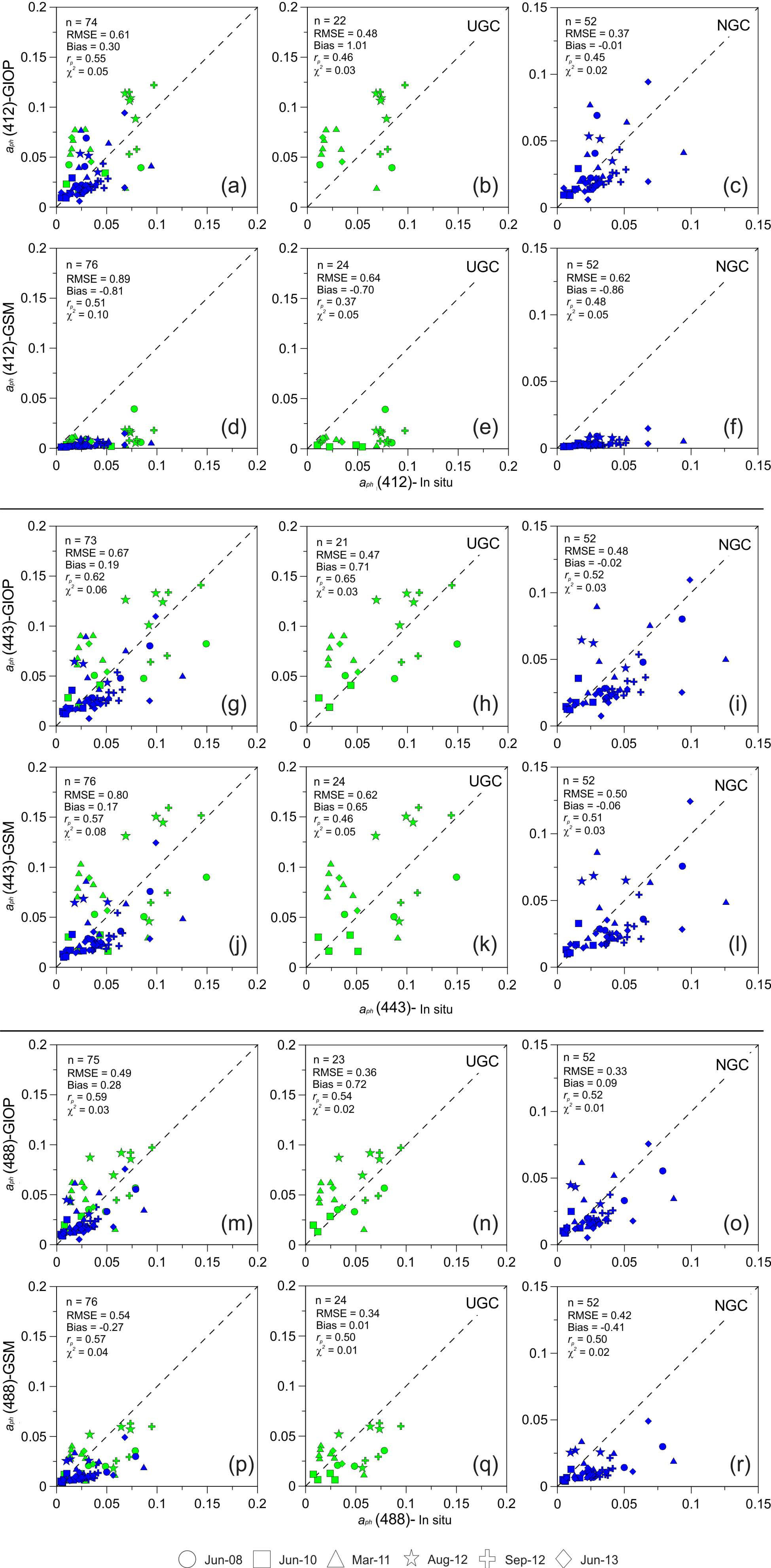
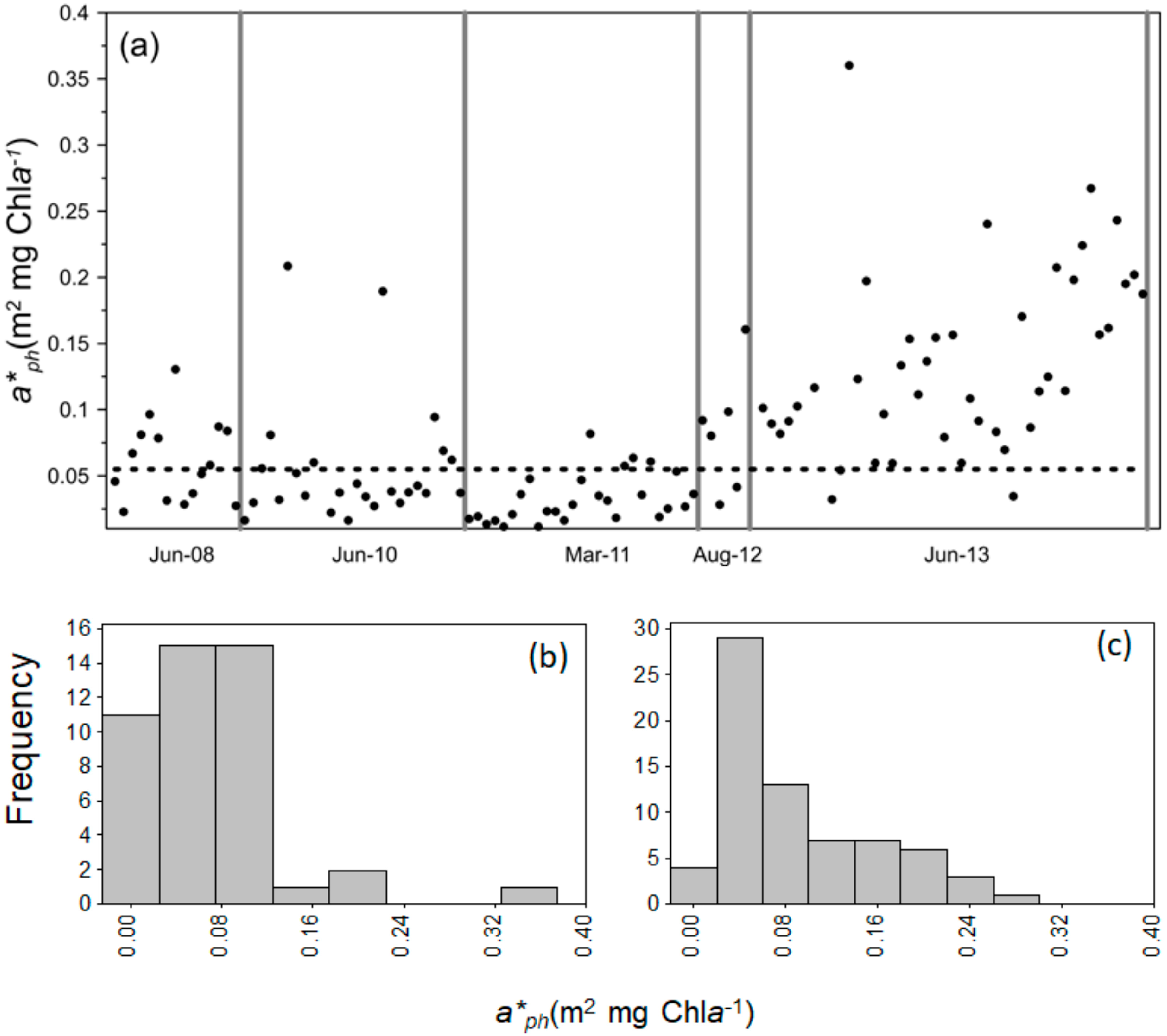
3.1. Phytoplankton Absorption Coefficient
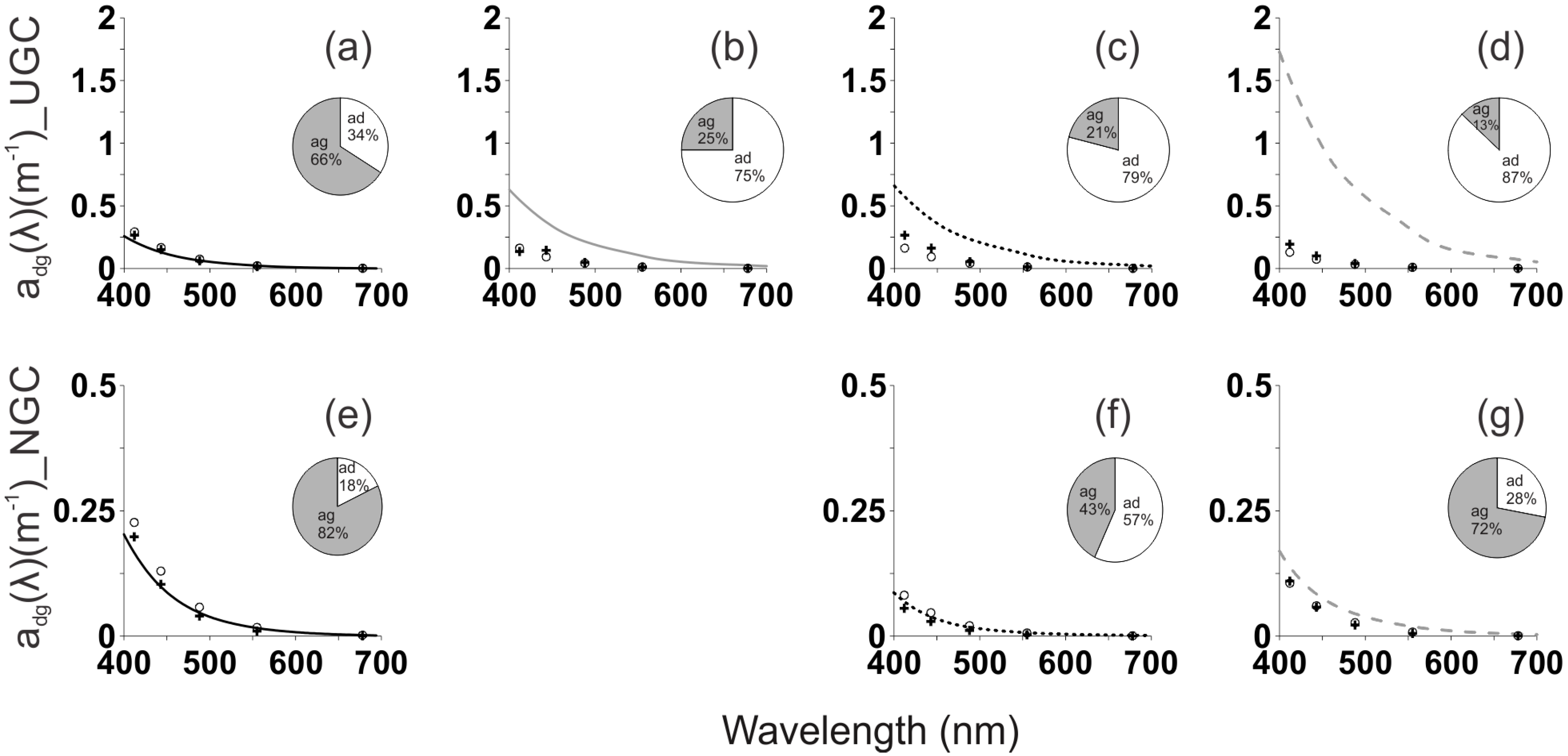
3.2. Absorption Coefficient of Dissolved and Detrital Matter
4. Conclusions
Supplementary Materials
Author Contributions
Funding
Acknowledgments
Conflicts of Interest
References
- McClain, C.R.; Cleave, M.L.; Feldman, G.C.; Gregg, W.W.; Hooker, S.B.; Kuring, N. Science Quality SeaWiFS Data for Global Biosphere Research. Available online: https://rsg.pml.ac.uk/staff/tjsm/sea_tech.html (accessed on 18 August 2017).
- McClain, C.R.; Christian, J.R.; Signorini, S.R.; Lewis, M.R.; Asanuma, I.; Turk, D.; Dupouy-Douchement, C. Satellite ocean-color observations of the tropical Pacific Ocean. Deep Sea Res. Part II Top. Stud. Oceanogr. 2002, 49, 2533–2560. [Google Scholar] [CrossRef]
- Gregg, W.W.; Conkright, M.E.; Ginoux, P.; O’Reilly, J.E.; Casey, N.W. Ocean primary production and climate: Global decadal changes. Geophys. Res. Lett. 2003, 30, 1809. [Google Scholar] [CrossRef]
- Behrenfeld, M.J.; Boss, E.; Siegel, D.A.; Shea, D.M. Carbon-based ocean productivity and phytoplankton physiology from space. Glob. Biogeochem. Cycles 2005, 19, GB1006. [Google Scholar] [CrossRef]
- Yoder, J.; Kennelly, M. What Have We Learned About Ocean Variability from Satellite Ocean Color Imagers? Oceanography 2006, 19, 152–171. [Google Scholar] [CrossRef]
- Garver, S.A.; Siegel, D.A. Inherent optical property inversion of ocean color spectra and its biogeochemical interpretation: 1. Time series from the Sargasso Sea. J. Geophys. Res. Oceans 1997, 102, 18607–18625. [Google Scholar] [CrossRef]
- Lee, Z.; Carder, K.L.; Steward, R.G.; Peacock, T.G.; Davis, C.O.; Patch, J.S. An empirical algorithm for light absorption by ocean water based on color. J. Geophys. Res. Oceans 1998, 103, 27967. [Google Scholar] [CrossRef]
- Carder, K.L.; Chen, F.R.; Lee, Z.P.; Hawes, S.K.; Kamykowski, D. Semianalytic Moderate-Resolution Imaging Spectrometer algorithms for chlorophyll a and absorption with bio-optical domains based on nitrate-depletion temperatures. J. Geophys. Res.Oceans 1999, 104, 5403–5421. [Google Scholar] [CrossRef]
- Morel, A.; Maritorena, S. Bio-optical properties of oceanic waters: A reappraisal. J. Geophys. Res. Oceans 2001, 106, 7163–7180. [Google Scholar] [CrossRef]
- Lee, Z.-P.; Darecki, M.; Carder, K.L.; Davis, C.O.; Stramski, D.; Rhea, W.J. Diffuse attenuation coefficient of downwelling irradiance: An evaluation of remote sensing methods. J. Geophys. Res. Oceans 2005, 110. [Google Scholar] [CrossRef]
- Lee, Z.-P.; Du, K.; Arnone, R.; Liew, S.; Penta, B. Penetration of solar radiation in the upper ocean: A numerical model for oceanic and coastal waters. J. Geophys. Res. Oceans 2005, 110. [Google Scholar] [CrossRef]
- Hu, C.; Lee, Z.; Muller-Karger, E.; Carder, L.; Walsh, J.J. Ocean color reveals phase shift between marine plants and yellow substance. IEEE Geosci. Remote Sens. Lett. 2006, 3, 262–266. [Google Scholar] [CrossRef]
- Capuzzo, E.; Painting, S.J.; Forster, R.M.; Greenwood, N.; Stephens, D.T.; Mikkelsen, O.A. Variability in the sub-surface light climate at ecohydrodynamically distinct sites in the North Sea. Biogeochemistry 2013, 113, 85–103. [Google Scholar] [CrossRef]
- Haraldsson, M.; Tönnesson, K.; Tiselius, P.; Thingstad, T.; Aksnes, D. Relationship between fish and jellyfish as a function of eutrophication and water clarity. Mar. Ecol. Prog. Ser. 2012, 471, 73–85. [Google Scholar] [CrossRef]
- Siegel, D.A.; Behrenfeld, M.J.; Maritorena, S.; McClain, C.R.; Antoine, D.; Bailey, S.W.; Bontempi, P.S.; Boss, E.S.; Dierssen, H.M.; Doney, S.C.; et al. Regional to global assessments of phytoplankton dynamics from the SeaWiFS mission. Remote Sens. Environ. 2013, 135, 77–91. [Google Scholar] [CrossRef]
- Brewin, R.J.; Sathyendranath, S.; Müller, D.; Brockmann, C.; Deschamps, P.-Y.; Devred, E.; Doerffer, R.; Fomferra, N.; Franz, B.; Grant, M. The Ocean Colour Climate Change Initiative: III. A round-robin comparison on in-water bio-optical algorithms. Remote Sens. Environ. 2013, 162, 271–294. [Google Scholar] [CrossRef]
- Mitchell, B.G.; Kahru, M.; Wieland, J.; Stramska, M.; Mueller, J.L. Determination of spectral absorption coefficients of particles, dissolved material and phytoplankton for discrete water samples. Ocean Opt. Protoc. Satell. Ocean Color Sens. Valid. Revis. 2002, 3, 231–257. [Google Scholar]
- Kirk, J.T. Light and Photosynthesis in Aquatic Ecosystems; Cambridge University Press: Cambridge, MA, USA, 1994. [Google Scholar]
- Lee, Z.P. Remote Sensing of Inherent Optical Properties: Fundamentals, Tests of Algorithms, and Applications; International Ocean-Colour Coordinating Group: Dartmouth, NS, Canada, 2006; Volume 5. [Google Scholar]
- Sathyendranath, S. Remote Sensing of Ocean Colour in Coastal, and Other Optically-Complex; IOCCG Report 3; IOCCG: Dartmouth, NS, Canada, 2000; p. 3. [Google Scholar]
- Maritorena, S.; Siegel, D.A.; Peterson, A.R. Optimization of a semianalytical ocean color model for global-scale applications. Appl. Opt. 2002, 41, 2705–2714. [Google Scholar] [CrossRef] [PubMed]
- Werdell, P.J.; Franz, B.A.; Bailey, S.W.; Feldman, G.C.; Boss, E.; Brando, V.E.; Dowell, M.; Hirata, T.; Lavender, S.J.; Lee, Z.; et al. Generalized ocean color inversion model for retrieving marine inherent optical properties. Appl. Opt. 2013, 52, 2019–2037. [Google Scholar] [CrossRef] [PubMed]
- Gordon, H.R.; Brown, O.B.; Evans, R.H.; Brown, J.W.; Smith, R.C.; Baker, K.S.; Clark, D.K. A semianalytic radiance model of ocean color. J. Geophys. Res. Atmos. 1988, 93, 10909–10924. [Google Scholar] [CrossRef]
- Lee, Z.; Carder, K.L.; Arnone, R.A. Deriving inherent optical properties from water color: A multiband quasi-analytical algorithm for optically deep waters. Appl. Opt. 2002, 41, 5755–5772. [Google Scholar] [CrossRef] [PubMed]
- Lee, Z.; Lubac, B.; Werdell, J.; Arnone, R. An Update of the Quasi-Analytical Algorithm (QAA_v5); IOCCG: Dartmouth, NS, Canada, 2009; pp. 1–9. [Google Scholar]
- Lee, Z.; Carder, K.L.; Mobley, C.D.; Steward, R.G.; Patch, J.S. Hyperspectral remote sensing for shallow waters. I. A semianalytical model. Appl. Opt. 1998, 37, 6329–6338. [Google Scholar] [CrossRef] [PubMed]
- Lavín, M.F.; Marinone, S.G. An overview of the physical oceanography of the Gulf of California. In Nonlinear Processes in Geophysical Fluid Dynamics; Velasco Fuentes, O.U., Sheibaum, J., Ochoa, J., Eds.; Springer: Dordrecht, The Netherlands, 2003; pp. 173–204. [Google Scholar]
- Bastidas-Salamanca, M.; González-Silvera, A.; Millán-Núñez, R.; Santamaría-del-Ángel, E.; Frouin, R. Bio-Optical Characteristics of the Northern Gulf of California during June 2008. Int. J. Oceanogr. 2014, 13. [Google Scholar] [CrossRef]
- Betancur-Turizo, S.P.; González-Silvera, A.G.; Santamaría-Del-Ángel, E.; Millán-Núñez, R.; Millán-Núñez, E.; García-Nava, H.; Godínez, V.M.; Sánchez-Velasco, L. Variability in the Light Absorption Coefficient by Phytoplankton, Non-Algal Particles and Colored Dissolved Organic Matter in the Northern Gulf of California. Open J. Mar. Sci. 2018, 8, 20–37. [Google Scholar] [CrossRef]
- Argote, M.L.; Amador, A.; Lavín, M.F.; Hunter, J.R. Tidal dissipation and stratification in the Gulf of California. J. Geophys. Res. Oceans 1995, 100, 16103–16118. [Google Scholar] [CrossRef]
- Hooker, S.B.; Clementson, L.; Thomas, C.S.; Schlüter, L. The HPLC Method, Chapter 6. In The Fifth SeaWiFS HPLC Analysis Round-Robin Experiment (SeaHARRE-5); NASA Technical Memorandum: Lanham, MD, USA, 2012; pp. 63–72. [Google Scholar]
- Werdell, P.J.; Franz, B.A.; Bailey, S.W.; Harding, L.W., Jr.; Feldman, G.C. Approach for the long-term spatial and temporal evaluation of ocean color satellite data products in a coastal environment. SPIE 2007, 6680, 66800G. [Google Scholar]
- Maritorena, S.; Siegel, D.A. Chapter 11: The GSM semi-analytical bio-optical model. Remote Sens. Inherent Opt. Prop. Fundam. Tests Algorithms Appl. 2006, 73–79. [Google Scholar]
- Santamaría-del-Ángel, E.; Millán-Núñez, R.; González-Silvera, A.; Cajal-Medrano, R. Comparison of In Situ and Remotely-Sensed Chl-a concentrations: A Statistical Examination of the Match-up Approach. In Handbook of Satellite Remote Sensing Image Interpretation: Applications for Marine Living Resources Conservation and Management; EU PRESPO Project: Wittibreut, Germany, 2010; pp. 221–238. [Google Scholar]
- Zar, H.H. Biostatistical Analysis, 4th ed.; Prentice Hall: Upper Saddle River, NJ, USA, 1999. [Google Scholar]
- Lee, Y.J.; Matrai, P.A.; Friedrichs, M.A.; Saba, V.S.; Aumont, O.; Babin, M.; Buitenhuis, E.T.; Chevallier, M.; De Mora, L.; Dessert, M. Net primary productivity estimates and environmental variables in the Arctic Ocean: An assessment of coupled physical-biogeochemical models. J. Geophys. Res. Oceans 2016, 121, 8635–8669. [Google Scholar] [CrossRef]
- Taylor, K.E. Summarizing multiple aspects of model performance in a single diagram. J. Geophys. Res. Atmos. 2001, 106, 7183–7192. [Google Scholar] [CrossRef]
- O’Reilly, J.E.; Maritorena, S.; Mitchell, B.G.; Siegel, D.A.; Carder, K.L.; Garver, S.A.; Kahru, M.; McClain, C. Ocean color chlorophyll algorithms for SeaWiFS. J. Geophys. Res. Oceans 1998, 103, 24937–24953. [Google Scholar] [CrossRef]
- O’Reilly, J.E.; Maritorena, S.; Siegel, D.A.; O’Brien, M.C.; Toole, D.; Mitchell, B.G.; Kahru, M.; Chavez, F.P.; Strutton, P.; Cota, G.F. Ocean color chlorophyll a algorithms for SeaWiFS, OC2, and OC4: Version 4. SeaWiFS Postlaunch Calibration Valid. Anal. 2000, 3, 9–23. [Google Scholar]
- Bricaud, A.; Claustre, H.; Ras, J.; Oubelkheir, K. Natural variability of phytoplanktonic absorption in oceanic waters: Influence of the size structure of algal populations. J. Geophys. Res. Oceans 2004, 109. [Google Scholar] [CrossRef]
- Jeffrey, S.W.; Mantoura, R.F.C.; Wright, S.W. Phytoplankton Pigments in Oceanography: Guidelines to Modern Methods; UNESCO Publishing: Paris, France, 1997; ISBN 978-92-3-103275-2. [Google Scholar]
- Millán-Núñez, E.; Sieracki, M.E.; Millán-Núñez, R.; Lara-Lara, J.R.; Gaxiola-Castro, G.; Trees, C.C. Specific absorption coefficient and phytoplankton biomass in the southern region of the California Current. Deep Sea Res. Part II Top. Stud. Oceanogr. 2004, 51, 817–826. [Google Scholar] [CrossRef]


| Cruises | Dates | Variables |
|---|---|---|
| June 2008 | 3–16 | aph(λ), ad(λ) |
| June 2010 | 1–10 | aph(λ), ad(λ) |
| March 2011 | 24 March to 1 April | aph(λ), ad(λ), aCDOM(λ) |
| August 2012 | 3–10 | aph(λ), ad(λ), aCDOM(λ) |
| September 2012 | 4–9 | aph(λ), ad(λ), aCDOM(λ) |
| June 2013 | 11–21 | aph(λ), ad(λ), aCDOM(λ) |
| Cruises | Total Stations | Julian Days | Total Days Per Cruise | Selected Level 1a Images |
|---|---|---|---|---|
| June 2008 | 22 | 158–164 | 6 | 11 |
| June 2010 | 30 | 152–159 | 8 | 8 |
| March 2011 | 27 | 84–91 | 8 | 10 |
| August 2012 | 10 | 216–223 | 8 | 3 |
| September 2012 | 30 | 248–253 | 6 | 6 |
| June 2013 | 46 | 162–171 | 9 | 10 |
| Total | 165 | 55 | 48 |
| Name | Description |
|---|---|
| ATMFAIL | Atmospheric correction failure |
| HIGLINT | High glint determined |
| HILT | High (or saturating) Top of the Atmosphere (TOA radiance) |
| HISATZEN | Large satellite zenith angle |
| STRAYLIGHT | Stray light determined |
| CLDICE | Probable cloud or ice contamination |
| LOWLW | Very low water-leaving radiance |
| MAXAERITER | Absorbing aerosols determined |
| λ | N | SDIn situ | SDSatellite | RMSE | Bias | Least Squares | |||||||
|---|---|---|---|---|---|---|---|---|---|---|---|---|---|
| GIOP | GIOP * | GIOP | GIOP * | GIOP | GIOP * | GIOP | GIOP * | GIOP | GIOP * | GIOP | GIOP * | ||
| UGC | 412 | 11 | 11 | 0.19 | 0.19 | 0.09 | 0.13 | 2.45 | 2.34 | −0.32 | −0.26 | 0.75 | 0.69 |
| 443 | 11 | 11 | 0.14 | 0.14 | 0.05 | 0.05 | 1.77 | 1.57 | −0.39 | −0.19 | 0.39 | 0.31 | |
| 488 | 11 | 8 | 0.09 | 0.10 | 0.02 | 0.01 | 1.18 | 1.04 | −0.51 | −0.42 | 0.18 | 0.13 | |
| NGC | 412 | 26 | 26 | 0.14 | 0.14 | 0.09 | 0.08 | 2.25 | 2.06 | 0.23 | 0.35 | 0.63 | 0.53 |
| 443 | 26 | 26 | 0.09 | 0.09 | 0.05 | 0.04 | 1.43 | 1.32 | 0.25 | 0.25 | 0.26 | 0.22 | |
| 488 | 26 | 26 | 0.05 | 0.05 | 0.02 | 0.02 | 0.76 | 0.72 | 0.19 | 0.02 | 0.07 | 0.06 | |
| λ | GSM | GSM * | GSM | GSM * | GSM | GSM * | GSM | GSM * | GSM | GSM * | GSM | GSM * | |
| UGC | 412 | 10 | 5 | 0.10 | 0.08 | 0.13 | 0.14 | 1.51 | 0.57 | −0.20 | −0.05 | 0.14 | 0.72 |
| 443 | 10 | 7 | 0.07 | 0.08 | 0.05 | 0.09 | 0.76 | 0.48 | −0.12 | 0.13 | 0.16 | 0.68 | |
| 488 | 7 | 5 | 0.05 | 0.06 | 0.01 | 0.04 | 0.54 | 0.16 | −0.35 | 0.09 | −0.25 | 0.88 | |
| NGC | 412 | 22 | 17 | 0.04 | 0.04 | 0.09 | 0.10 | 1.12 | 1.02 | 0.54 | 0.41 | 0.53 | 0.59 |
| 443 | 22 | 18 | 0.03 | 0.03 | 0.05 | 0.06 | 0.55 | 0.67 | 0.42 | 0.60 | 0.54 | 0.67 | |
| 488 | 22 | 16 | 0.02 | 0.01 | 0.02 | 0.04 | 0.21 | 0.34 | 0.17 | 0.51 | 0.52 | 0.79 | |
© 2018 by the authors. Licensee MDPI, Basel, Switzerland. This article is an open access article distributed under the terms and conditions of the Creative Commons Attribution (CC BY) license (http://creativecommons.org/licenses/by/4.0/).
Share and Cite
Betancur-Turizo, S.P.; González-Silvera, A.; Santamaría-del-Ángel, E.; Tan, J.; Frouin, R. Evaluation of Semi-Analytical Algorithms to Retrieve Particulate and Dissolved Absorption Coefficients in Gulf of California Optically Complex Waters. Remote Sens. 2018, 10, 1443. https://doi.org/10.3390/rs10091443
Betancur-Turizo SP, González-Silvera A, Santamaría-del-Ángel E, Tan J, Frouin R. Evaluation of Semi-Analytical Algorithms to Retrieve Particulate and Dissolved Absorption Coefficients in Gulf of California Optically Complex Waters. Remote Sensing. 2018; 10(9):1443. https://doi.org/10.3390/rs10091443
Chicago/Turabian StyleBetancur-Turizo, Stella Patricia, Adriana González-Silvera, Eduardo Santamaría-del-Ángel, Jing Tan, and Robert Frouin. 2018. "Evaluation of Semi-Analytical Algorithms to Retrieve Particulate and Dissolved Absorption Coefficients in Gulf of California Optically Complex Waters" Remote Sensing 10, no. 9: 1443. https://doi.org/10.3390/rs10091443
APA StyleBetancur-Turizo, S. P., González-Silvera, A., Santamaría-del-Ángel, E., Tan, J., & Frouin, R. (2018). Evaluation of Semi-Analytical Algorithms to Retrieve Particulate and Dissolved Absorption Coefficients in Gulf of California Optically Complex Waters. Remote Sensing, 10(9), 1443. https://doi.org/10.3390/rs10091443