Article

Evaluation of the Stability of the Darbandikhan Dam after the 12 November 2017 Mw 7.3 Sarpol-e Zahab (Iran–Iraq Border) Earthquake

1
School of Engineering, Newcastle University, Newcastle upon Tyne NE1 7RU, UK
2
COMET, School of Engineering, Newcastle University, Newcastle upon Tyne NE1 7RU, UK
*
Authors to whom correspondence should be addressed.
Remote Sens. 2018, 10(9), 1426; https://doi.org/10.3390/rs10091426
Submission received: 19 July 2018 / Revised: 2 September 2018 / Accepted: 5 September 2018 / Published: 7 September 2018
(This article belongs to the Special Issue Imaging Geodesy and Infrastructure Monitoring)

Abstract

:
We used a global positioning system (GPS), levelling, and Sentinel-1 data to evaluate the stability of the Darbandikhan dam in northeast Iraq after the 2017 Mw 7.3 Sarpol-e Zahab earthquake. GPS and levelling datasets collected in March and November 2017 were used to compute the co-seismic surface displacements of the dam. Sentinel-1 synthetic aperture radar (SAR) images collected between October 2014 and March 2018 were employed to recover the displacement time series of the dam. The large-magnitude displacement gradient on the dam crest hindered the estimation of the co-seismic displacement using this medium-resolution SAR data. However, Sentinel-1 images are sufficient to examine the stability of the dam displacement before and after the earthquake. The results show that the dam was stable between October 2014 and November 2017, but after the earthquake, Sentinel-1 data shows a continuous subsidence of the dam crest between November 2017 and March 2018. To the best knowledge of the authors, this study is the first that utilises InSAR to investigate the behaviour of a dam after a large earthquake.

Graphical Abstract

1. Introduction

The 12 November 2017 Sarpol-e Zahab earthquake was one of the largest earthquakes occurring in the Iran–Zagros zone since 1900 [1]. About 396 lives were lost, and 7000 people were injured on both sides of Iraq–Iran border [2], with the majority of fatalities occurring in the Iranian city of Sarpol-e Zahab, whereas Darbandikhan was the most impacted city in Iraq. The earthquake struck the northeast of Iraq, with its epicentre 30 km away from the Darbandikhan dam (Figure 1), and there is now serious concern about the Darbandikhan dam’s safety. The dam was previously evaluated to be seismically safe under a maximum probable shaking of Mw 6.5 [3]. According to the map of the shaking intensity from the United States (US) Geological Survey (USGS) (Figure 1b), the dam lies within the region of 8 MMI (modified Mercalli intensity) for the 2017 event. Following this earthquake, the dam operators immediately lowered the water level in the reservoir because of concern about the dam’s safety. The deformation of the dam body after the earthquake is visually apparent, and the State Commission on the Survey of Iraq observed several fissures on the crest soon afterwards. In the following months, this region exhibited 53 aftershocks with Mw > 4.
Dams can be affected by earthquakes with several different types of deterioration, including: (1) slope failure; (2) cross-sectional and longitudinal cracks; (3) seepage from the foundation and the side slopes; (4) liquefaction of the dam body; (5) freeboard reduction; and (6) overtopping due to waves in the reservoir [6,7].
The response of earth fill and rockfill dams to earthquakes differs according to the acceleration and velocity of the motion [8], and also depends on the geological setting of the dam [9]. The most important factor that may affect the man-made infrastructure during an earthquake is the velocity of shaking [8]. When the acceleration is sufficiently large, the shaking causes a temporary downslope movement, which may reach 1.5 m [10]. Another critical factor is the construction quality. Dams with a low degree of compaction are most susceptible to damage by earthquakes. The crest of the dam is the most vulnerable part during a seismic event, as its slopes can temporarily slide towards the toe of the dam. The failure of the dam can lead to permanent displacements along the slope and may extend to the whole surface or just part of the dam slope [11]. Some notable dams were damaged by earthquakes with Mw > 6, e.g., the Sheffield Dam in 1925 and the San Andreas Dam in 1906 (both in California, US). Seco and Pedro [7] reviewed several case studies of dam deformation following earthquakes, based on the history of embankment dams selected from all over the world. Not far away from the Darbandikhan dam, the Mosul dam threatened millions of people living downstream, and interferometric SAR (InSAR) has been used to detect its instability after the political instability of the area in 2014 [12]. The early detection of the instability of the Mosul dam with InSAR led to a maintenance plan to stabilize the foundation of the dam before it turned into a disaster [13,14]. The worst scenario of dam failure triggered by an earthquake was the loss of 100,000 lives during the landslides following the 1786 Kangding–Luding Mw 7.7 earthquake, which struck Sichuan, southwest China [15]. Newmark (1965) discussed the mechanics of the dam structure during successive shakings. He suggested three possible movements of the dam: (1) dam slope motion either in the upstream or downstream direction; (2) creep of the whole dam in a specific direction; and (3) relative motion between the structural parts, which may lead to fissures in the dam body. The third is the most problematic, because it may be followed by internal erosion [9].
Although the Darbandikhan dam lies in an active seismic region, there is no seismic instrumentation in the dam to monitor its behaviour during and after earthquakes. A previous concern about the safety of the dam was reported in [3]. This detailed report discussed the importance of monitoring the dam grouting gallery, as water seepage was observed here on more than one occasion [3]. Furthermore, it was reported that there was further concern about a landslide in the left bank and rock fill from the cliffs in the right and left abutments of the dam. Thus, there were some efforts to implement a maintenance plan between 2006 and 2010.
In this paper, we attempt to use geodetic observations (i.e., GPS, levelling and InSAR) to examine the stability of the Darbandikhan dam before and after the 2017 Mw 7.3 Sarpol-e Zahab earthquake. The paper starts with a brief description of the geological setting of the dam in Section 2. Section 3 outlines the methodology used in the monitoring, including a description of the geodetic monitoring system, the principles of InSAR, and the limitations of small baseline subset (SBAS) InSAR to monitor the slopes of the dam. The results from geodetic and InSAR techniques are presented in Section 4, followed by a discussion of the main findings in Section 5. A summary and conclusions of the study are presented in Section 6.

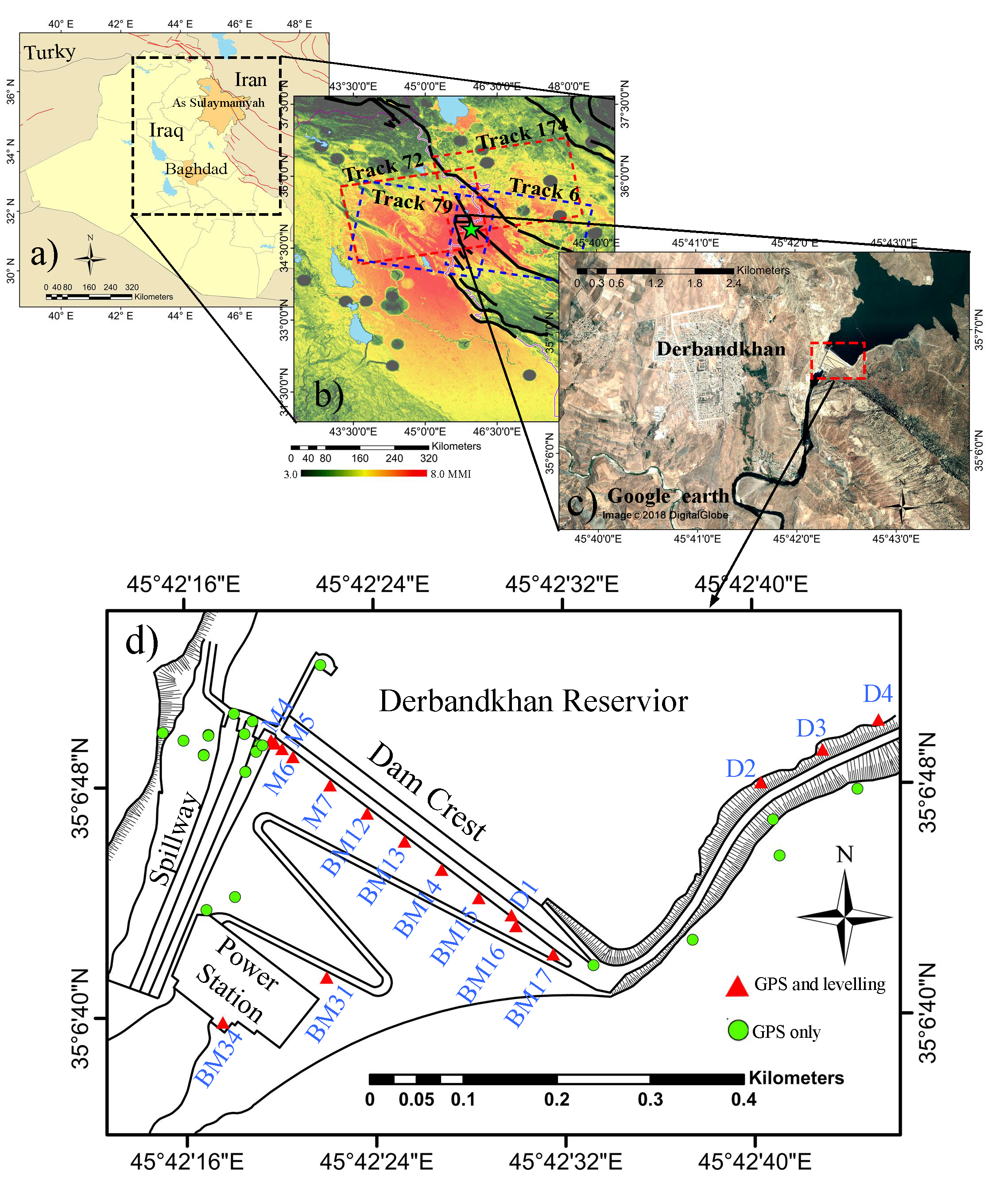
2. Geological Setting

The Darbandikhan dam was constructed between 1956–1961 on the Diyala Sirwan river, 230 km northeast of Baghdad and 65 km southeast of Sulaimaniyah province. Its location was selected to span the gorge formed by the intersection of the Daila river and Branand Dagh anticline. Four main geological units can be found in the area: Qarah Chauq Limestone, Green Marl Formation, Buff Formation, and Bituminous Marl Formation. The last two strata make up the dam foundation, and the core and downstream shoulder of the dam are founded on the Buff Formation [3].
The dam is located close to the collision between the Arabian and Eurasian tectonic plates in the Zagros collision zone [16]. According to Binnie et al. (1987), the dam was designed to withstand earthquakes with a maximum Mw of 6.5. The dam structure is a clay core rock-fill dam with a maximum height above the foundation of 128 m. The gradients of both the upstream and downstream slopes are 30°, and the length and width of the crest are 535 m and 17 m, respectively.
The reservoir holds three billion cubic meters of water, which is used for irrigation and power generation. According to the dam design, the water level in the reservoir should be maintained between 455–485 m. However, these limits were exceeded several times to meet the demands of the hydro station [3]. The elevation of the spillway ogee is 470 m, which allows discharge of 5700 m3/s to 11,400 m3/s when the reservoir water level varies between 485–493.5 m, respectively.

3. Methods

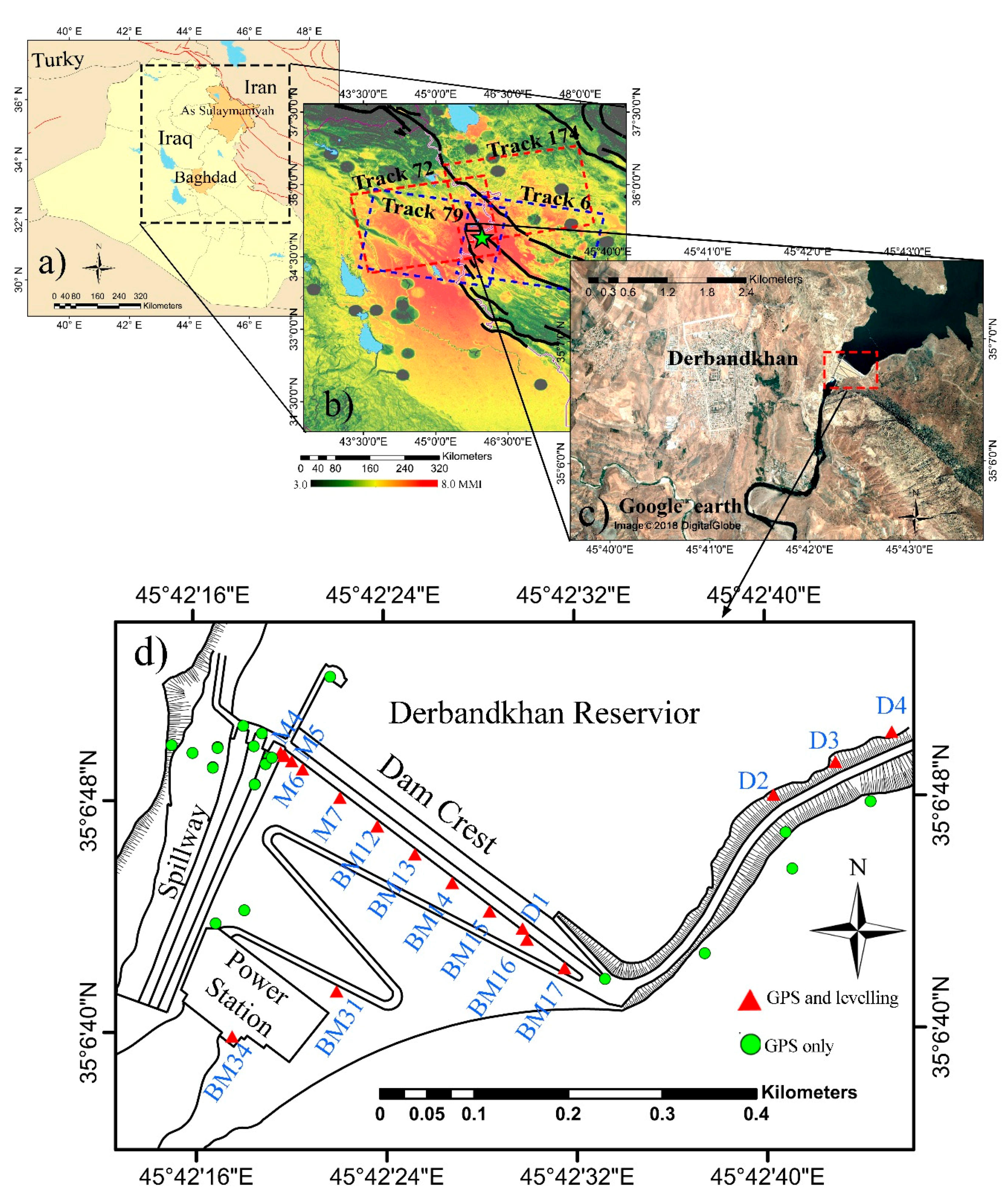
3.1. Dam Instrumentation
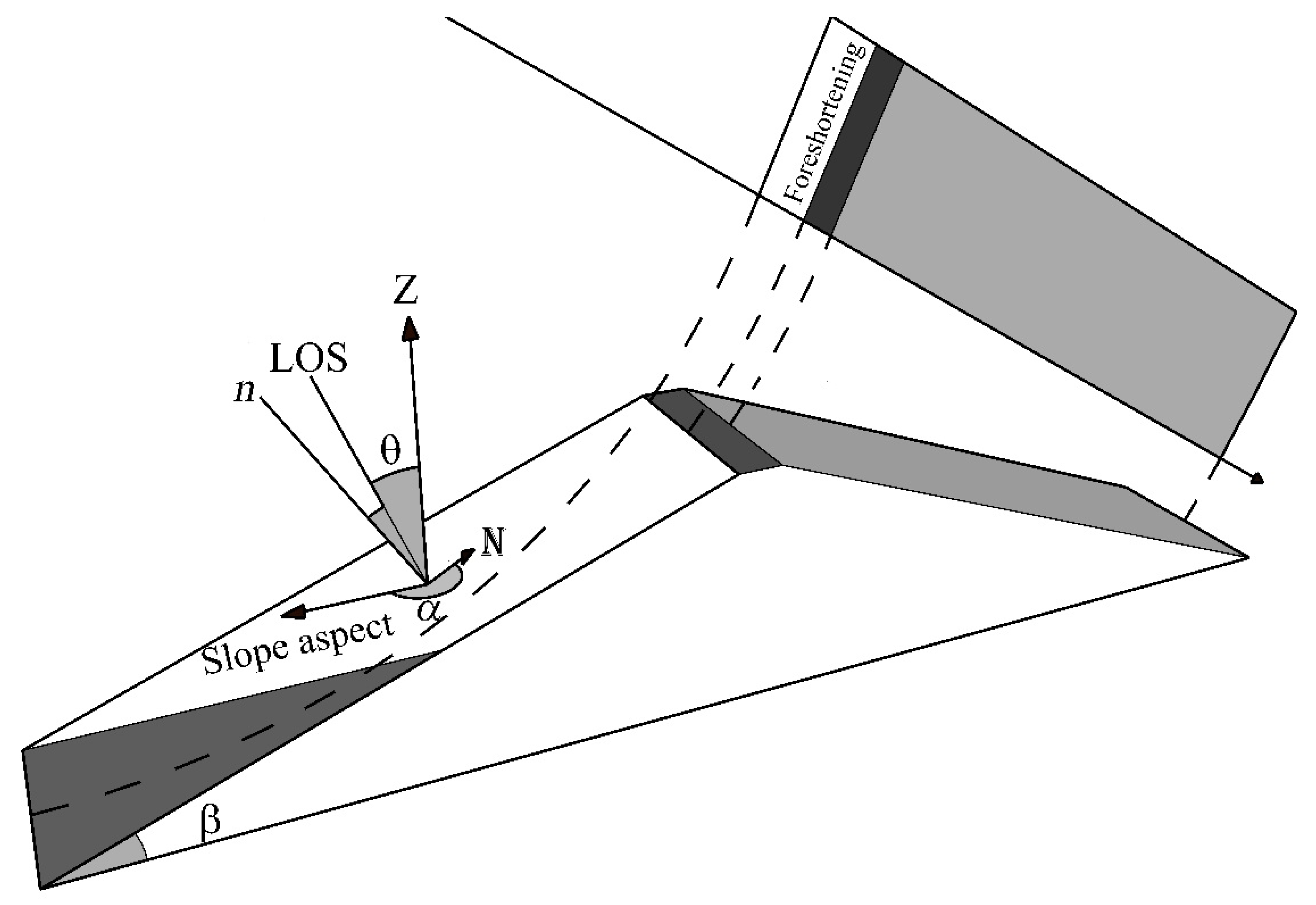
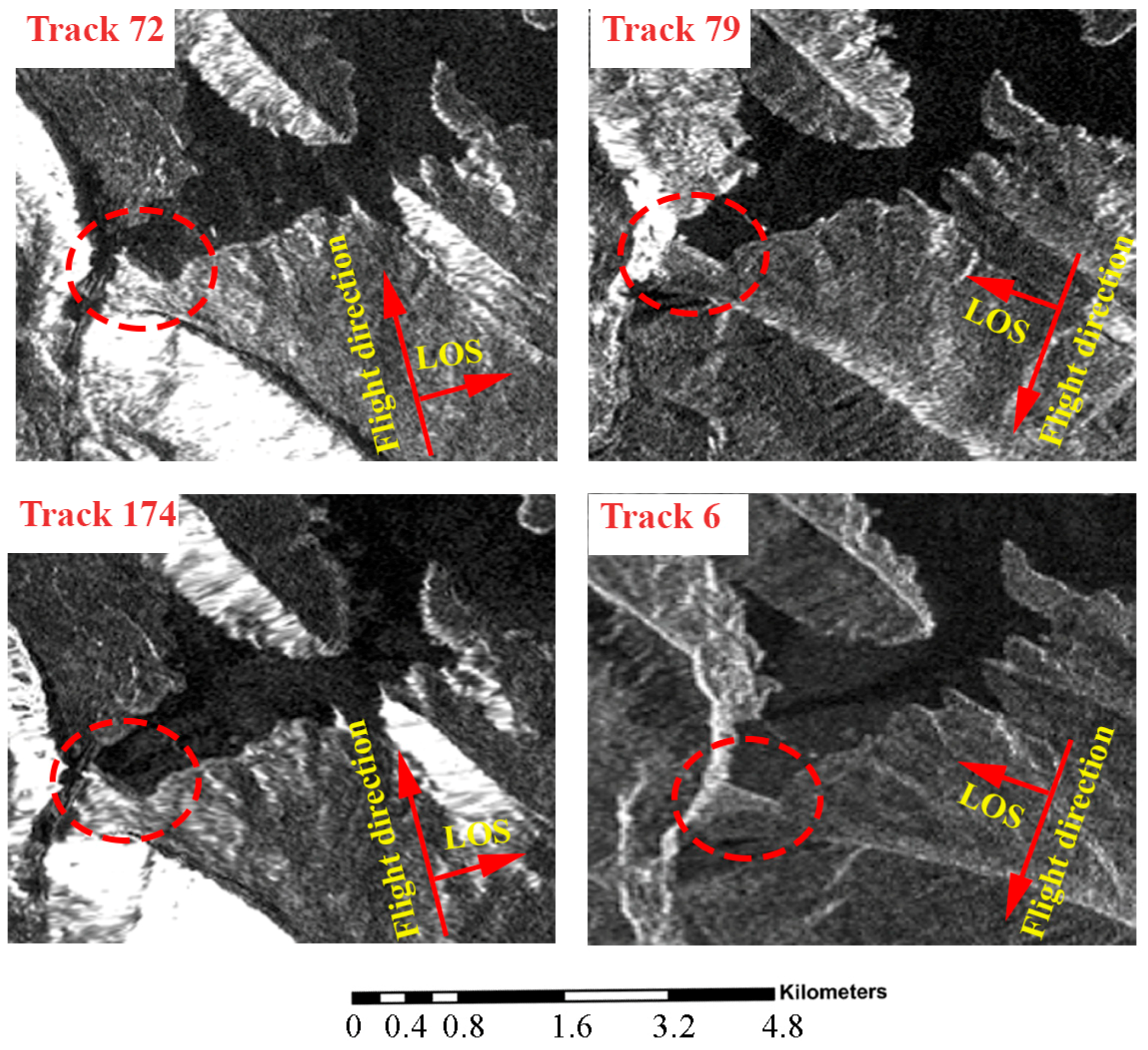
The safety of Darbandikhan dam is inspected periodically by the Ministry of Water Resources/State Commission of Survey of Iraq by observing a geodetic network to detect any abnormal behaviour. Figure 1d illustrates the monitoring pillars of the dam, which are used in this study. This network consists of pillars installed on the dam surface, where regular GPS and levelling observations are taken, as well as levelling stations within the inspection gallery for which no relevant data are available. Only two epochs of GPS and levelling data, collected in March and November 2017, were available for this study. To plot a displacement profile of the dam crest and for analysis purposes, we consider the left edge of the spillway head (Station M4) as the reference. This is also applicable for calculating the gradient of displacement in Section 3.2.
Water seepage was monitored by nine piezometers installed in the dam body, and 23 piezometers installed in the gallery. Readings of the core piezometers taken during two periods—(i) from 1976 to 1978 and (ii) from January 1980 to May 1981—indicated normal behaviour of the dam [3]. The reservoir water level is monitored by a floating instrument installed close to the power station intake. The accuracy of the reading is ±10 mm.

3.2. InSAR

InSAR with multiple SAR images is able to determine small movements of the ground, which are in the order of millimeters when the conditions are preferable. The applications of the InSAR technique date back to the 1970s [17,18,19] and the first spaceborne SAR mission, SEASAT, was launched in 1978 for estimating ocean waves [20]. With the increase of the number of spaceborne radar missions, InSAR has developed rapidly in the last two decades. The imaging specifications in terms of spatial and temporal resolution have improved significantly, and this has contributed to remarkable expansion in the applications of InSAR. Spaceborne InSAR has been successfully applied for large-scale applications such as topographic mapping [21,22,23,24,25,26,27,28], earthquake deformation [19,29,30,31,32], volcano monitoring [33,34,35,36,37,38], landslides [39,40,41,42,43,44], and even for generic nationwide InSAR deformation mapping [45]. Recently, SENTINEL-1 SAR data have been used for the dynamic monitoring of ground displacement [46,47] and to forecast the landslide time of failure [48]. Nevertheless, the surveillance of mass-wasting phenomena characterized by a high displacement rate or impulsive triggers is possible only using ground-based sensors as GBInSAR devices [48,49,50,51,52]
The rapid development of InSAR processing algorithms and imaging specifications has encouraged researchers to utilise InSAR to monitor the stability of dams [53,54,55,56,57,58]. Here, we utilised Sentinel-1 InSAR data for monitoring the post-seismic movement of the Darbandikhan dam.
A total of 68 Sentinel-1 images from Track 6 were collected over the Darbandikhan dam. One of the limitations of using InSAR for dam monitoring is the foreshortening of the side slopes, which may result in underestimation of the deformation magnitude. Images of objects in the SAR images are projected to the line of sight (LOS) of the radar beam. Consequently, the distances of the dam slopes and crests appear to be shorter than their actual values by a factor depending on the SAR geometry and slope aspect. First, we investigated this compression factor, which is the ratio between slant and ground ranges, for the upstream and downstream slope in each track. The compression factor can be calculated as follows [44,59]:
  R = sin ( ϑ β · sin ( A ) )  
where ϑ is the incidence angle of radar signals, β is the dam side slope, and A is the aspect correction factor, which can be computed from the aspect of the slope (α) and the satellite heading angle (ϒ). A = α − ϒ for the ascending pass, and A = α + ϒ + 180° for the descending pass [59]. The parameters of Equation (1) are shown in Figure 2. Table 1 shows the compression ratios for different tracks of Sentinel-1 data on the upstream and downstream slopes of the dam. Over the downstream slope, tracks 72, 79, and 174 are more influenced by foreshortening than track 6, so we used images from track 6 only in this study. The same calculations over the upstream slope show that the foreshortening on the upstream slope is much more than that on the downstream slope. Although the upstream slope is often covered by water, the water level was reduced to a shallower level after the 12 November 2017 earthquake, and so part of this slope is now visible.
According to Cigna et al [59], R takes values between 0 and 1 for each pixel on the dam surface. R = 0 when the LOS is perpendicular to the sloping surface, and R = 1 when the LOS is parallel to it. All of the pixels on a level surface, such as pixels on the dam crest, have:
  R = sin ( ϑ )  
This is yielded by considering β = 0 in Equation (1). Thus, for pixels on the dam crest, R = 0.55 for the ascending pass, and R = 0.69 in the descending pass.
In Figure 3, the dam is indicated with red circles. The downstream slope of the dam and the terrain slopes facing to the radar LOS, look brighter than the other areas in the single-look complex (SLC) image. This is because the foreshortening increases the radar intensity (having more backscatter returned into a single pixel yield more intensity); the foreshortening factor R for slopes facing the radar is smaller than that for the slopes facing away from the radar LOS. Although tracks 72 and 174 are from the same ascending pass, those slopes look brighter in track 72. This is because the SLC image subset in Figure 3 is located in the far range of track 72, while it is in the near range of track 174. In other words, their incidence angles are different, leading to different foreshortening impacts.
Another limitation of InSAR is the difficulty of retrieving the LOS displacement when it exceeds the maximum detectable gradient [41,49]. This limitation comes from an assumption that is made at the stage of phase unwrapping. This assumption is that the difference in the LOS phase changes between two adjacent pixels is less than π/2, which is equivalent to a difference of λ/4 in the LOS range changes because of the two-way travel path of the radar signals. To investigate the reliability of using Sentinel-1 for such large magnitude displacements, we computed the gradient along the LOS by simulating the LOS displacement from the levelling and GPS measurement on the dam crest using the following equation:
  L O S d i s = E G sin ϑ sin φ + N G sin ϑ cos φ + U L cos ϑ  
where LOSdis is the projection of the three-dimensional (3D) displacement vector [EG NG UL] to the LOS vector. EG and NG are the easting and northing components derived from GPS, UL is the vertical component obtained from levelling, and ϑ and φ are the incidence angle of the radar LOS and the azimuth of the satellite flight, respectively. The spatial resolution of the SAR images can be a critical parameter in cases of steep gradients of displacement [41]. To evaluate the feasibility of the Sentinel-1 spatial resolution for such localised displacement over short distances (less than 500 m), the gradient of LOS displacement between every pair of adjacent benchmarks on the dam crest is computed by dividing the difference of their LOS displacements by the horizontal distance between them. Table 2 shows the computations of the simulated LOS displacement of Track 6 and the gradient between every pair of adjacent pillars on the dam crest.
Assuming the pixel size of the interferograms generated from Sentinel-1A/B is ≈20 m and the surface is completely flat (knowing that all of the benchmarks M4 to BM17 in Table 2 are on the crest), the maximum detectable gradient (MDG) of displacement is:
  M D G = λ 4 D × R  
where λ is the wavelength of the SAR system (0.0555 m for Sentinel-1), D is the pixel size, and R is the compression factor. Thus, the maximum detectable gradient is ≈1 mm/m, which is less than the LOS displacement gradient between all of the benchmarks on the dam crest, as shown in Table 2. In Table 2, the maximum gradient is 3 mm/m between M6 and M7. Thus, the minimum resolution required to detect this displacement is λ/4 g, which amounts to 4.57 m. In other words, when using data with a spatial resolution less than 4.57 m, it is impossible to recover such a large gradient displacement signal, which is evidenced by all of the co-seismic interferograms (e.g., Figure S1) generated in this study. Here, we assume that the unwrapping path will follow the topmost part of the crest where the apparent displacement gradient is smallest. For points on the slope, the apparent displacement gradient G will be:
  G = g / R  
where g is the actual displacement gradient, and R is the compression factor. On the downstream slope, the gradient of the displacement will be significantly larger, because R is at most 0.69, and hence unwrapping errors are likely, hindering any estimation of co-seismic displacement using Sentinel-1 data. Following a different unwrapping path with a steeper gradient would require a spatial resolution better than 4.57 m. The High-Resolution Spotlight or the Starring Spotlight (ST) acquisition modes of TerraSAR-X are the most suitable to recover such large-gradient co-seismic displacements, but these were unavailable for our study. Consequently, Sentinel-1 data was used only to investigate the dam surface displacements before and after the earthquake, whereas the co-seismic displacements were estimated from GPS and levelling data.
The GAMMA software [60] was used for InSAR processing. Two constraints were applied to select the interferograms: (i) the perpendicular baseline should not exceed 400 m, and (ii) the time separation of the two SAR acquisitions should be less than 180 days. All of the SLC images were co-registered to one master. The differential interferograms were filtered using the adaptive filtering algorithm [61]. This step was performed to increase the signal-to-noise ratio in some incoherent pixels so as to reduce the likelihood of unwrapping errors in the next step. The differential interferograms were unwrapped using the minimum cost network flow two-dimensional (2D) unwrapping method [62,63]. The surface displacement time series and the mean linear velocities for each pixel were generated using the in-house InSAR TS+AEM software, which essentially employs the small baseline subset (SBAS) approach [64]. Recent studies suggest that tropospheric delay products from external datasets such as the Global Navigation Satellite System (GNSS) and European Centre for Medium-Range Weather Forecasts (ECMWF) can be used to reduce the atmospheric effects on radar measurements [65,66], which can, in turn, facilitate time series analysis [67,68]. However, due to the small extent of the dam, we did not expect large spatial variations in the atmospheric water vapour. Thus, no such external information was used to mitigate atmospheric effects.

4. Results

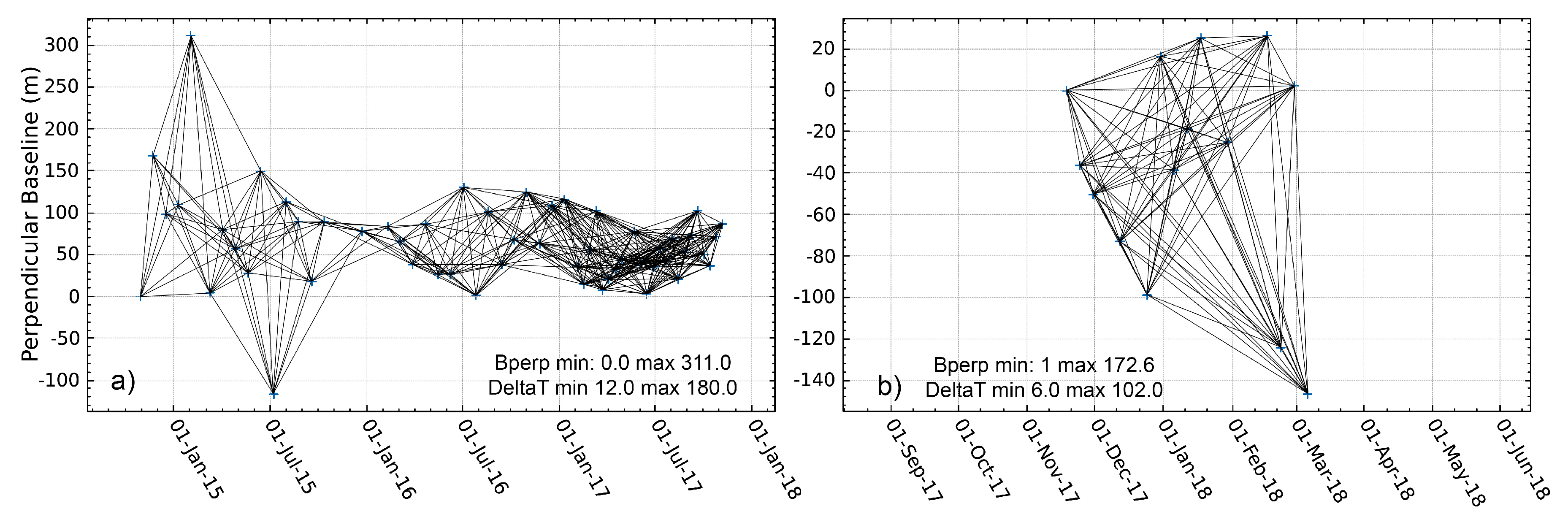
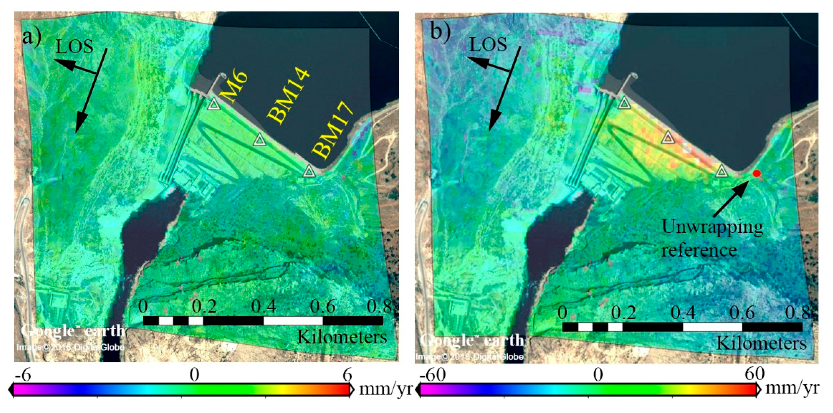
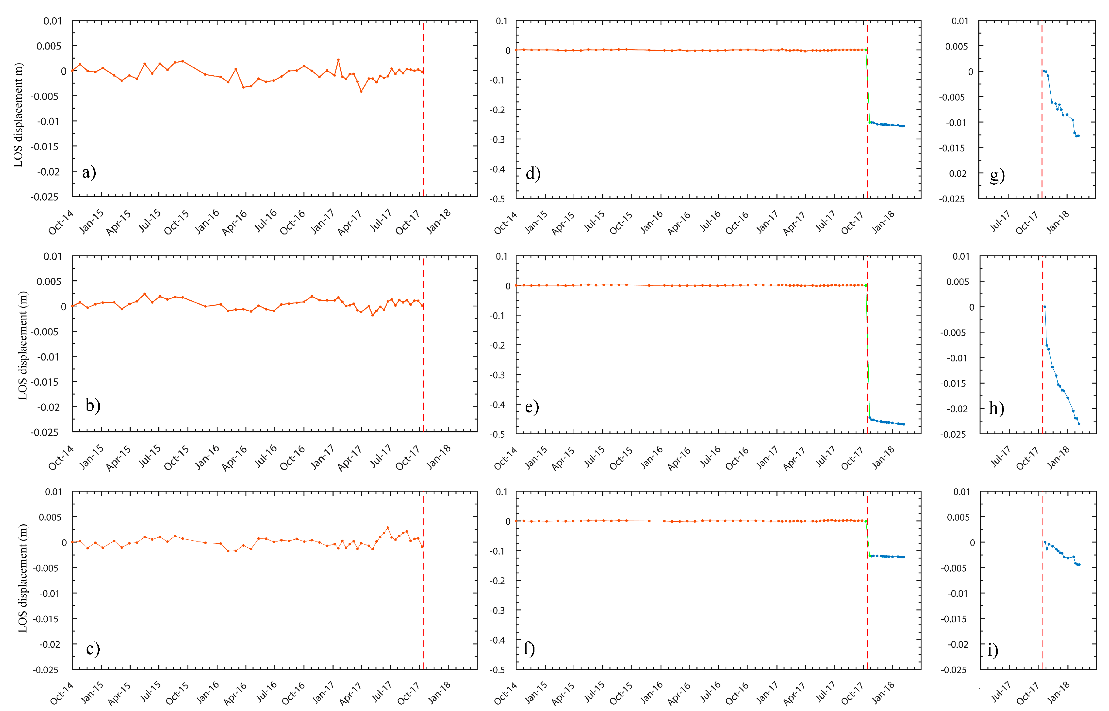
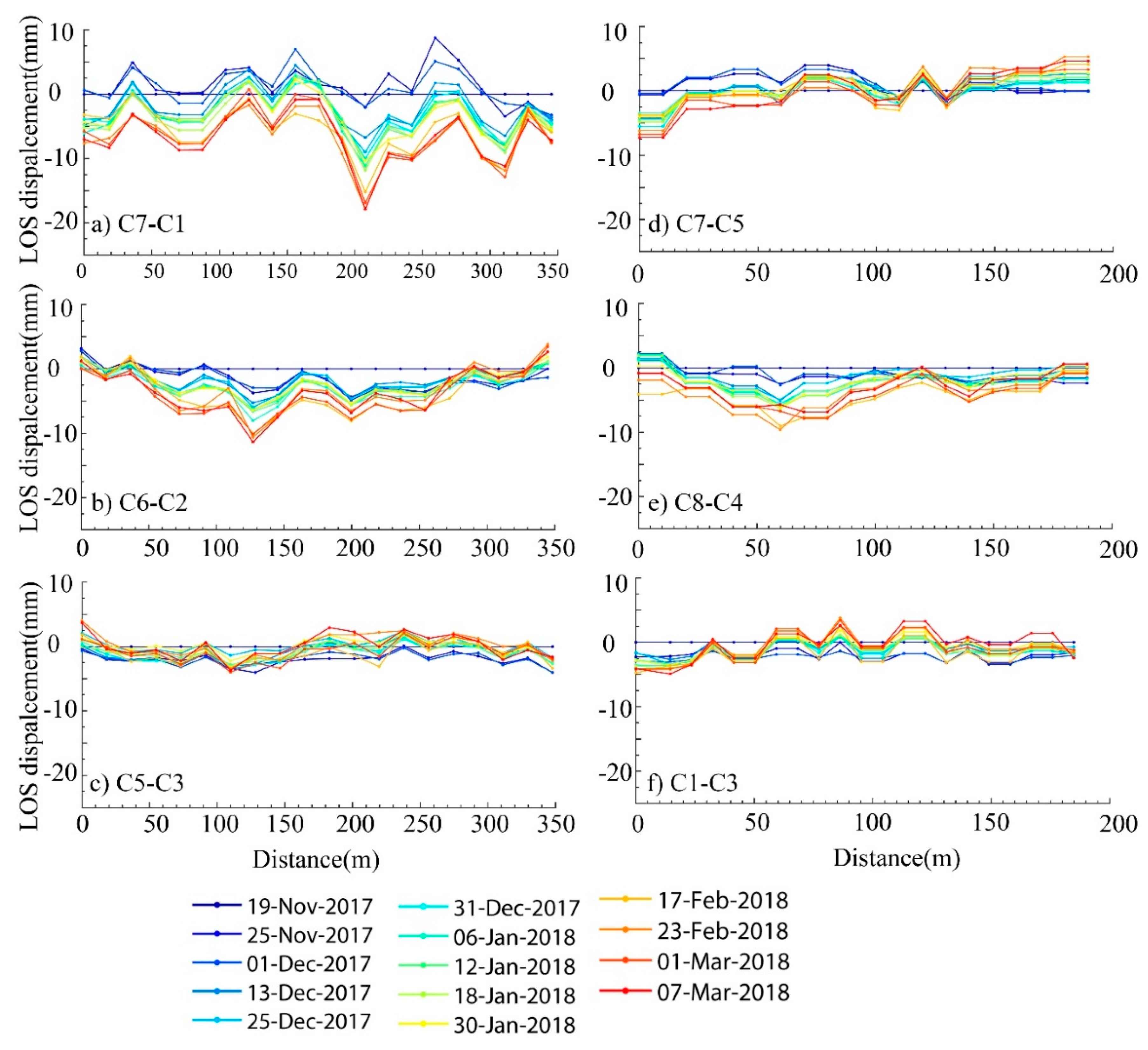
4.1. InSAR Time Series

To investigate the behaviour of the dam before and after the earthquake, we generated the displacement time series using 68 Sentinel-1 A/B images collected between October 2014 and March 2018. Only acquisitions from track 6 were used to generate the SBAS time series, because they are less distorted, as discussed in Section 3.2. We separated the time series into two time spans. Figure 4 shows the spatial–temporal separation of the acquisition for each time span. For the pre-seismic period between October 2014 and 7 November 2017, we generated the SBAS time series using 54 Sentinel-1 images. Figure 5a shows the mean LOS velocity map of the dam before the earthquake. The maximum rate of displacement of any point on the dam crest, with respect to the phase unwrapping origin point on bedrock just to the east of the dam (Figure 5b), is 4 mm/year during this period. Note that the apparent uplift across areas of higher topography away from the dam most likely represents residual atmospheric effects that are unrelated to deformation across the dam, and can be neglected. The time series error map is shown in Figure S3a in the supplementary material.
Figure 5b shows the post-seismic LOS velocity map using 14 Sentinel-1A/B images between 19 November 2017 and 7 March 2018. The error map of the SBAS time series is presented in Figure S3b in the supplementary material. To connect the pre-event and post-event time series at the monitoring pillars on the dam crest, we estimated the LOS displacement for each benchmark from GPS and levelling data using Equation (3). Figure 6 illustrates the LOS displacement time series of three points on the dam crest—M6, BM14, and BM17—which are indicated in Figure 5a. BM14 is located close to the centre of the dam, and the other two are on the western and eastern edges, respectively. It can be seen that the dam was stable before the earthquake, but there is a rapid displacement of BM14 after 11 November 2017, and it is clear that the dam crest is continuously moving, even four months after the earthquake, with a 17-mm LOS displacement of BM14 between 19 November 2017 and 7 March 2018.

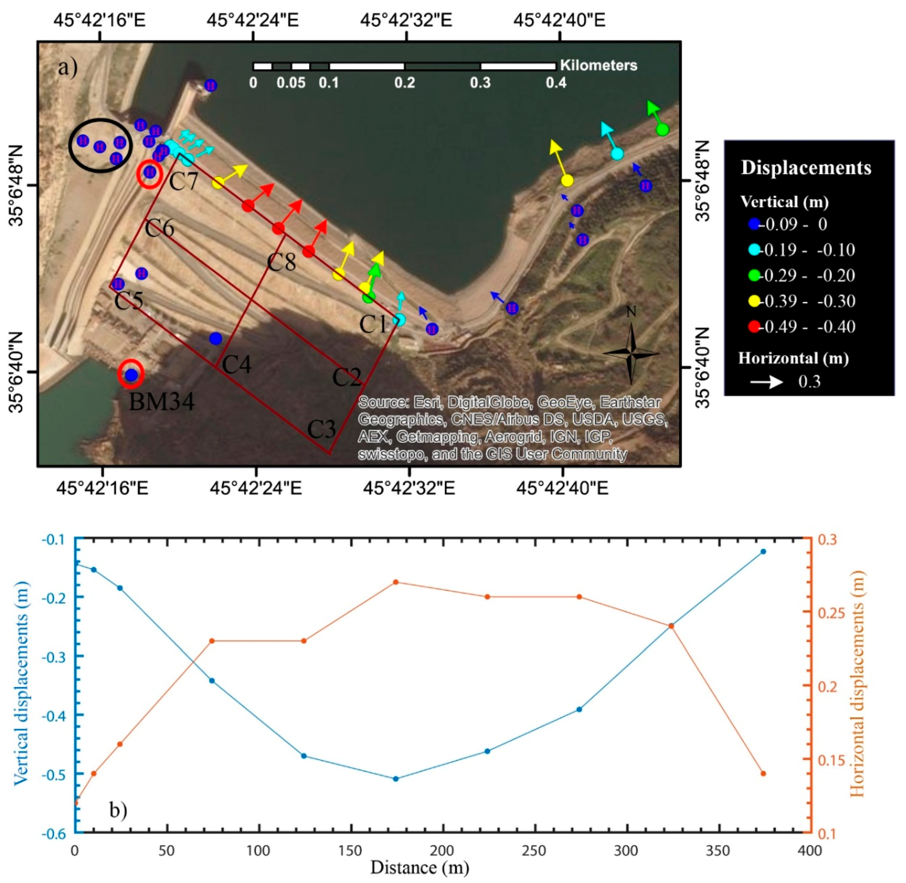
4.2. Co-Seismic Displacement from GPS and Levelling Measurements
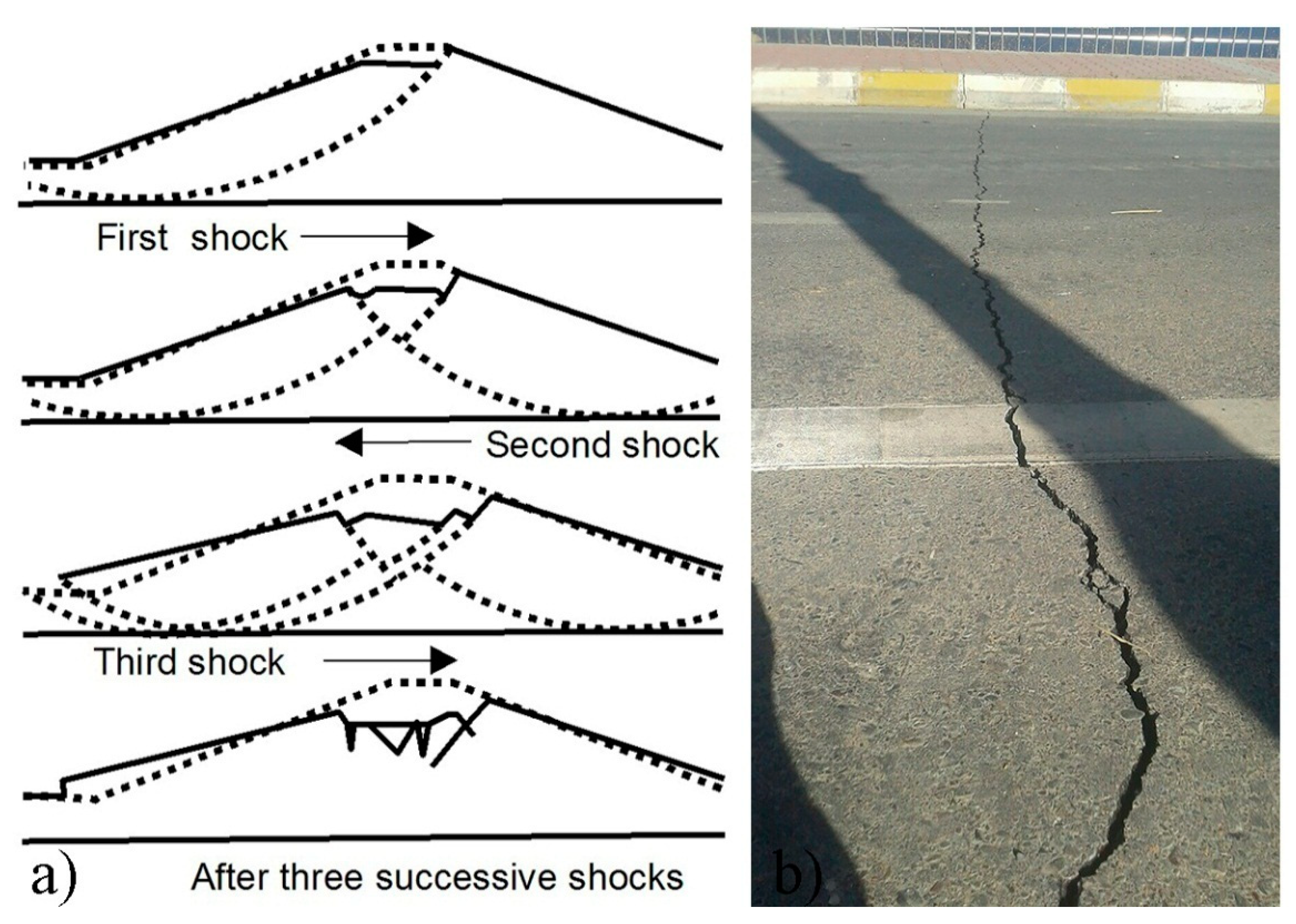
The first GPS and levelling campaign was carried out in March 2017, and the second was carried out in November 2017. Figure S2 shows the absolute co-seismic displacements relative to ITRF08. Four stable points (indicated by a black oval) outside the dam body and close to the spillway moved by a similar magnitude to the spillway head and the dam toe (both indicated by red circles). The average horizontal displacement of these four stable points is approximately 0.12 m in the southwest direction, which represents the absolute co-seismic movement of the dam and its surrounding area. It is well-known that relative movements are more crucial in terms of dam safety. Therefore, the average displacement of the four stable points away from the dam body, which are indicated by the black oval in Figure S2, is subtracted from the dam movements. Figure 7 shows the vertical and horizontal relative displacements of the dam crest and its spillway measured by GPS and levelling after subtracting this average horizontal movement. The maximum relative horizontal displacement measured by GPS is 0.27 m at station BM13. The relative horizontal displacements of the left and right abutments are around 0.14 m and 0.12 m, respectively. It can be seen that the pattern of displacement of all of the points on the crest tends towards the centreline of the dam. The pillars near the centre of the dam moved perpendicular to the dam axis, while points on the right and the left of the dam moved in the northeast and northwest directions, respectively.
The relative vertical displacement measured by the levelling is shown as coloured scale circles in Figure 7a, and depicted as a blue vertical profile in Figure 7b. The subsidence of the central part of the dam is more than 0.50 m. The vertical displacements of the points on the left and right abutments range from 0.15 m to 0.45 m.

5. Discussion

The LOS mean velocity maps in Figure 5, which were derived from the InSAR time series, show different patterns of settlement on the left and right parts of the dam. It is understood that the water level in the reservoir was lowered immediately after the earthquake, which could be the reason why there was no water seepage crossing the dam body at that stage. The emergence of cracks on the downstream side slope can be more dangerous than those upstream or on the crest. No crack has yet been observed on the downstream slope of the Darbandikhan dam, but minor cracks could be hiding beneath the boulder-covered face of the slope due to the difficulty of observing cracks in such a surface.
It is clear in Figure 7 that different parts of the dam displaced with different magnitudes in both the vertical and horizontal directions, although the maximum displacement is focussed in the centre. As suggested by Newmark [8] and Herndon [69], such behaviours are expected for Earth fill dams during an earthquake. Shaking the embankment of the dam results in the non-uniform displacement of different parts of the embankment, depending on the acceleration. Figure 8a shows one plausible mechanism of the Earth fill dam movement after three successive shocks [8]. The direction of the shaking may impact the magnitude of the displacement, while the movement must be along the slope aspect in spite of the direction of the shaking, because of the gravity. In addition, the slope in the centre of the dam is expected to be longer than the left and right sides, suggesting a V section of the bedrock along the dam axis. This suggestion is evidenced by the gallery design that was constructed along the dam axis following the bedrock and leaving 75 m of the dam section without any gallery [3]. We expect that this section was left without the gallery because the bedrock along the river section is too steep, which may hinder the construction of the gallery in this section. Therefore, the most affected part of the dam is the crest, and maximum deformation can be observed close to the dam centre when the embankment height and the slope length are maximum. This behaviour is evidenced by several cracks that appeared on the left and right abutment of the Darbandikhan dam after the earthquake. Figure 8b shows one of the major cracks crossing the dam axis located in the left abutment.
According to Cordell et al. [3], the dam’s surrounding area exhibited several landslide events in the past. The GPS displacement vectors above the reservoir to the east of the dam show consistent downslope local movements. Thus, continuous monitoring of the area is essential, especially given that the region exhibited several minor aftershock events. Higher-resolution radar images (e.g., TerraSAR-X and COSMO-SkyMED) are desirable for monitoring the upstream dam slope, which is expected to move more than the downstream slope, according to the GPS and levelling data.
Figure 9 shows six displacement cross-sections derived from the SBAS InSAR time series between November 2017 and March 2018. The location of each cross-section is depicted in Figure 7a. Figure 9a–c are cross-sections that are parallel to the dam axis, arranged from the top to the toe of the dam, respectively. As inferred from the GPS and levelling, the topmost section shows the greatest displacement. Figure 9d–f show the displacement on three cross-sections along the downstream slope that are arranged from the west to east abutment, respectively. Figure 9e is along the centreline of the slope, and similarly shows the greatest displacement at the dam crest.

6. Conclusions

In this study, we investigated the impact of the Mw 7.3 Sarpol-e Zahab earthquake on the deformation of the Darbandikhan dam in northeast (NE) Iraq. We used three geodetic techniques to investigate the dam movements before, after, and during the earthquake. Due to the steep gradients of the co-seismic displacements, GPS and levelling measurements were utilised to observe the distortion of the dam body caused by the earthquake, suggesting movements of up to 270 mm in the horizontal direction and 500 mm in the vertical direction. We discussed the limitations of using InSAR techniques for monitoring sloping surfaces, and the spatial and temporal resolution required to recover large-gradient displacements. The rate of the dam displacement before and after the earthquake was investigated using InSAR time series analysis with 68 Sentinel-1 images collected between October 2014 and March 2018. Our results suggest that the dam was relatively stable before the event, with a maximum LOS velocity of 4 mm/year, but after the event, the crest of the dam was still creeping at a rate of up to 70 mm/year until at least March 2018. These results suggest that spaceborne InSAR monitoring of the post-seismic dam deformation is useful to inform maintenance plans, but that episodic terrestrial surveys remain essential in case of large-gradient deformation during future earthquakes.

Supplementary Materials

The following are available online at https://www.mdpi.com/2072-4292/10/9/1426/s1, Figure S1. Co-seismic interferogram (7 November 2017–19 November 2017): (a) Interferogram, and (b) Coherence. Derbandkhan dam is indicated with white oval. Figure S2. The horizontal (indicated by arrows) and vertical (indicated by circles) displacements of the monitoring pillars on Derbandkhan dam measured by GPS and levelling. The source of the background image is from [5]. Note that (i) the horizontal displacements are referenced to ITRF08, and (ii) the pillars labelled with letter H were measured with GPS only. Figure S3. The corresponding error maps of the mean linear velocity maps in Figure 4a,b respectively. Note that the error maps show the RMS differences between InSAR derived displacements and a temporally linear deformation model. Table S1. Acquisition dates of Tracks, 6, 79, 72 and 174.

Author Contributions

Y.A.-H. and Z.L. conceived and designed the experiments; Y.A.-H. performed the experiments under the supervision of Z.L., P.C. and S.E.; the whole team analyzed the data; Y.A.-H. drafted the paper and all the co-authors contributed to the writing.

Acknowledgments

This work was supported by the Ministry of Higher Education/University of Wasit and the Ministry of Water resources/State Commission of Survey, Iraq. Part of this work was also supported by the UK NERC through the Centre for the Observation and Modelling of Earthquakes, Volcanoes and Tectonics (COMET, ref.: COME30001) and the LICS project (ref. NE/K010794/1), and by the ESA-MOST DRAGON-4 project (ref. 32244). We thank the Copernicus Sentinel data [2018] for Sentinel-1 data, and the State Commission of Survey and Ministry of Water Resources in Iraq for GPS and levelling data.

Conflicts of Interest

The authors declare no conflict of interest.

References

  1. Alsinawi, S.; Ghalib, H. Historical seismicity of Iraq. Bull. Seismol. Soc. Am. 1975, 65, 541–547. [Google Scholar]
  2. BBC News Middle East. Iran-Iraq earthquake: Hundreds killed as border region hit. BBC News Middle East, 13 November 2017. [Google Scholar]
  3. Cordell, M.C. Dokan and Derbendikhan Dam Inspections; SMEC International Pty. Ltd.: Malvern East, Australia, 2006. [Google Scholar]
  4. USGS (2017) Interactive map. 13 November 2017. Available online: https://earthquake.usgs.gov/earthquakes/eventpage/us2000bmcg#map (accessed on 13 November 2017).
  5. ESRI. DigitalGlobe, GeoEye, Earthstar Geographics, CNES/Airbus DS, USDA, USGS, AEX, Getmapping, Aerogrid, IGN, IGP, Swisstopo, and the GIS User Community; ESRI: Redlands, CA, USA, 2018. [Google Scholar]
  6. Jansen, R.B. Dams and Public Safety (A Water Resources Technical Publication); United States Government Printing Office; U.S. Department of the Interior, Bureau of Reclamation Interior, U.S.D: Denver, CO, USA, 1983.
  7. Seco, E.P.; Pedro, S. Understanding Seismic Embankment Dam Behavior Through Case Histories. In Proceedings of the International Conferences on Recent Advances in Geotechnical Earthquake Engineering and Soil Dynamics, San Diego, CA, USA, 24–29 May 2010. [Google Scholar]
  8. Newmark, N.M. Effects of Earthquakes on Dams and Embankments. Géotechnique 1965, 15, 139–160. [Google Scholar] [CrossRef]
  9. Anastasiadis, A.; Klimis, N.; Makra, K.; Margaris, B. On seismic behavior of a 130m high rockfill dam: An integrated approach. In Proceedings of the 13th World Conference on Earthquake Engineering, Vancouver, BC, Canada, 1–6 August 2004. [Google Scholar]
  10. Serff, N.; Seed, H.B.; Makdisi, F.I.; Chang, C.-Y. Earthquake-Induced Deformations of Earth Dams; EERC 76-4; College of Engineering; University of Claifornia: Oakland, CA, USA, 1976; pp. 9–10. [Google Scholar]
  11. Jansen, R.B.; Parrett, N.F.; Ingram, D.E. Safety Evaluation of Existing Dams; United Department of the Interior Bureau of Reclamation: Denever, CO, USA, 1995. [Google Scholar]
  12. Milillo, P.; Bürgmann, R.; Lundgren, P.; Salzer, J.; Perissin, D.; Fielding, E.; Biondi, F.; Milillo, G. Space geodetic monitoring of engineered structures: The ongoing destabilization of the Mosul dam, Iraq. Sci. Rep. 2016, 6, 37408. [Google Scholar] [Green Version]
  13. Trevi. Trevi Signs the Contract for the Maintenance Works of Mosul Dam. 2018. Available online: http://www.trevispa.com/en/MosulDam/trevi-signs-the-contract-for-the-maintenance-works-of-mosul-dam (accessed on 18 July 2018).
  14. Annunziato, A.; Andredakis, I.; Probst, P. Impact of Flood by a Possible Failure of the Mosul Dam; EUR 27923 EN; European Commission: Brussels, Belgium, 2016. [Google Scholar]
  15. Dai, F.C.; Lee, C.F.; Deng, J.H.; Tham, L.G. The 1786 earthquake-triggered landslide dam and subsequent dam-break flood on the Dadu River, southwestern China. Geomorphology 2005, 65, 205–221. [Google Scholar] [CrossRef]
  16. Sadeghi, S.; Yassaghi, A. Spatial evolution of Zagros collision zone in Kurdistan, NW Iran: Constraints on Arabia-Eurasia oblique convergence. Solid Earth 2016, 7, 659–672. [Google Scholar] [CrossRef]
  17. Bills, B.G.; Ferrari, A.J. A harmonic analysis of lunar topography. Icarus 1977, 31, 244–259. [Google Scholar] [CrossRef]
  18. Zisk, S. A new, earth-based radar technique for the measurement of lunar topography. Earth Moon Planets 1972, 4, 296–306. [Google Scholar] [CrossRef]
  19. Gabriel, A.K.; Goldstein, R.M.; Zebker, H.A. Mapping small elevation changes over large areas: Differential radar interferometry. J. Geophys. Res. Solid Earth 1989, 94, 9183–9191. [Google Scholar] [CrossRef]
  20. Jordan, R. The Seasat-A synthetic aperture radar system. IEEE J. Ocean. Eng. 1980, 5, 154–164. [Google Scholar] [CrossRef]
  21. Zebker, H.A.; Villasenor, J.; Madsen, S.N. Topographic Mapping From ERS-1 And Seasat Radar Interferometry. In Proceedings of the IGARSS ’92 International Geoscience and Remote Sensing Symposium, Houston, TX, USA, 26–29 May 1992; pp. 387–388. [Google Scholar]
  22. Ferretti, A.; Prati, C.; Rocca, F.; Monti Guarnieri, A. Multibaseline SAR Interferometry for Automatic DEM Reconstruction (DEM). In Proceedings of the Third ERS Symposium on Space at the Service of our Environment, Florence, Italy, 14–21 March 1997. [Google Scholar]
  23. Farr, T.G.; Rosen, P.A.; Caro, E.; Crippen, R.; Duren, R.; Hensley, S.; Kobrick, M.; Paller, M.; Rodriguez, E.; Roth, L.; et al. The Shuttle Radar Topography Mission. Rev. Geophys. 2007, 45. [Google Scholar] [CrossRef] [Green Version]
  24. Krieger, G.; Moreira, A.; Fiedler, H.; Hajnsek, I.; Werner, M.; Younis, M.; Zink, M. TanDEM-X: A Satellite Formation for High-Resolution SAR Interferometry. IEEE Trans. Geosci. Remote Sens. 2007, 45, 3317–3341. [Google Scholar] [CrossRef] [Green Version]
  25. Liao, M.; Wang, T.; Lu, L.; Zhou, W.; Li, D. Reconstruction of DEMs From ERS-1/2 Tandem Data in Mountainous Area Facilitated by SRTM Data. IEEE Trans. Geosci. Remote Sens. 2007, 45, 2325–2335. [Google Scholar] [CrossRef]
  26. Wegmüller, U.; Santoro, M.; Werner, C.; Strozzi, T.; Wiesmann, A.; Lengert, W. DEM generation using ERS–ENVISAT interferometry. J. Appl. Geophys. 2009, 69, 51–58. [Google Scholar] [CrossRef]
  27. Neelmeijer, J.; Motagh, M.; Bookhagen, B. High-resolution digital elevation models from single-pass TanDEM-X interferometry over mountainous regions: A case study of Inylchek Glacier, Central Asia. ISPRS J. Photogramm. Remote Sens. 2017, 130, 108–121. [Google Scholar] [CrossRef] [Green Version]
  28. Ebmeier, S.K.; Biggs, J.; Mather, T.A.; Elliott, J.R.; Wadge, G.; Amelung, F. Measuring large topographic change with InSAR: Lava thicknesses, extrusion rate and subsidence rate at Santiaguito volcano, Guatemala. Earth Planet. Sci. Lett. 2012, 335–336, 216–225. [Google Scholar] [CrossRef]
  29. Massonnet, D.; Feigl, K.; Rossi, M.; Adragna, F. Radar interferometric mapping of deformation in the year after the Landers earthquake. Nature 1994, 369, 227–230. [Google Scholar] [CrossRef]
  30. Polcari, M.; Palano, M.; Fernández, J.; Samsonov, S.V.; Stramondo, S.; Zerbini, S. 3D displacement field retrieved by integrating Sentinel-1 InSAR and GPS data: The 2014 South Napa earthquake. Eur. J. Remote Sens. 2017, 49, 1–13. [Google Scholar] [CrossRef]
  31. Avallone, A.; Cirella, A.; Cheloni, D.; Tolomei, C.; Theodoulidis, N.; Piatanesi, A.; Briole, P.; Ganas, A. Near-source high-rate GPS, strong motion and InSAR observations to image the 2015 Lefkada (Greece) Earthquake rupture history. Sci. Rep. 2017, 7, 10358. [Google Scholar] [CrossRef] [PubMed]
  32. Ganas, A.; Kourkouli, P.; Briole, P.; Moshou, A.; Elias, P.; Parcharidis, I. Coseismic Displacements from Moderate-Size Earthquakes Mapped by Sentinel-1 Differential Interferometry: The Case of February 2017 Gulpinar Earthquake Sequence (Biga Peninsula, Turkey). Remote Sens. 2018, 10, 1089. [Google Scholar] [CrossRef]
  33. Rosen, P.A.; Hensley, S.; Zebker, H.A.; Webb, F.H.; Fielding, E.J. Surface deformation and coherence measurements of Kilauea Volcano, Hawaii, from SIR-C radar interferometry. J. Geophys. Res. Ser. 1996, 101. [Google Scholar] [CrossRef]
  34. Beauducel, F.; Briole, P.; Froger, J.-L. Volcano-wide fringes in ERS synthetic aperture radar interferograms of Etna (1992–1998): Deformation or tropospheric effect? J. Geophys. Res. Solid Earth 2000, 105, 16391–16402. [Google Scholar] [CrossRef]
  35. Remy, D.; Bonvalot, S.; Briole, P.; Murakami, M. Accurate measurements of tropospheric effects in volcanic areas from SAR interferometry data: Application to Sakurajima volcano (Japan). Earth Planet. Sci. Lett. 2003, 213, 299–310. [Google Scholar] [CrossRef]
  36. Spaans, K.; Hooper, A. InSAR processing for volcano monitoring and other near-real time applications. J. Geophys. Res. Solid Earth 2016, 121, 2947–2960. [Google Scholar] [CrossRef] [Green Version]
  37. Thomas, A.; Holley, R.; Burren, R.; Shilston, D.; Waring, D.; Meikle, C. Long-term differential InSAR monitoring of the Lampur Sidoarjo mud volcano (Java, Indonesia) using ALOS PALSAR imagery. In Proceedings of the 8th International Symposium on Land Subsidence, Querétaro, Mexico, 17–22 October 2010. [Google Scholar]
  38. Biggs, J.B.; Ebmeier, S.K.; Aspinall, W.P.; Lu, Z.; Pritchard, M.E.; Sparks, R.S.; Mather, T.A. Global link between deformation and volcanic eruption quantified by satellite imagery. Nat. Commun. 2014, 5, 3471. [Google Scholar] [CrossRef] [PubMed] [Green Version]
  39. Ferretti, A.; Prati, C.; Rocca, F.; Casagli, N.; Farina, P.; Young, B. Permanent Scatterers technology: A powerful state of the art tool for historic and future monitoring of landslides and other terrain instability phenomena. In Proceedings of the 2005 International Conference on Landslide Risk Management, Vancouver, BC, Canada, 31 May–3 June 2005. [Google Scholar]
  40. Bozzano, F.; Cipriani, I.; Mazzanti, P.; Prestininzi, A. Displacement patterns of a landslide affected by human activities: Insights from ground-based InSAR monitoring. Nat. Hazards 2011, 59, 1377–1396. [Google Scholar] [CrossRef]
  41. Singleton, A.; Li, Z.; Hoey, T.; Muller, J.P. Evaluating sub-pixel offset techniques as an alternative to D-InSAR for monitoring episodic landslide movements in vegetated terrain. Remote Sens. Environ. 2014, 147, 133–144. [Google Scholar] [CrossRef]
  42. Tomás, R.; Li, Z.; Liu, P.; Singleton, A.; Hoey, T.; Cheng, X. Spatiotemporal characteristics of the Huangtupo landslide in the Three Gorges region (China) constrained by radar interferometry. Geophys. J. Int. 2014, 197, 213–232. [Google Scholar] [CrossRef] [Green Version]
  43. Dai, K.; Li, Z.; Tomás, R.; Liu, G.; Yu, B.; Wang, X.; Cheng, H.; Chen, J.; Stockamp, J. Monitoring activity at the Daguangbao mega-landslide (China) using Sentinel-1 TOPS time series interferometry. Remote Sens. Environ. 2016, 186, 501–513. [Google Scholar] [CrossRef]
  44. Darvishi, M.; Schlögel, R.; Bruzzone, L.; Cuozzo, G. Integration of PSI, MAI, and Intensity-Based Sub-Pixel Offset Tracking Results for Landslide Monitoring with X-Band Corner Reflectors—Italian Alps (Corvara). Remote Sens. 2018, 10, 409. [Google Scholar] [CrossRef]
  45. Novellino, A.; Cigna, F.; Brahmi, M.; Sowter, A.; Bateson, L.; Marsh, S. Assessing the Feasibility of a National InSAR Ground Deformation Map of Great Britain with Sentinel-1. Geosciences 2017, 7, 19. [Google Scholar] [CrossRef]
  46. Raspini, F.; Bianchini, S.; Ciampalini, A.; Del Soldato, M.; Solari, L.; Novali, F.; Del Conte, S.; Rucci, A.; Ferretti, A.; Casagli, N. Continuous, semi-automatic monitoring of ground deformation using Sentinel-1 satellites. Sci. Rep. 2018, 8, 7253. [Google Scholar] [CrossRef] [PubMed]
  47. Amelung, F.; Galloway, D.L.; Bell, J.W.; Zebker, H.A.; Laczniak, R.J. Sensing the ups and downs of Las Vegas: InSAR reveals structural control of land subsidence and aquifer-system deformation. Geology 1999, 27, 483. [Google Scholar] [CrossRef]
  48. Intrieri, E.; Gigli, G.; Nocentini, M.; Lombardi, L.; Mugnai, F.; Fidolini, F.; Casagli, N. Sinkhole monitoring and early warning: An experimental and successful GB-InSAR application. Geomorphology 2015, 241, 304–314. [Google Scholar] [CrossRef] [Green Version]
  49. Di Traglia, F.; Intrieri, E.; Nolesini, T.; Bardi, F.; Del Ventisette, C.; Ferrigno, F.; Frangioni, S.; Frodella, W.; Gigli, G.; Lotti, A.; et al. The ground-based InSAR monitoring system at Stromboli volcano: Linking changes in displacement rate and intensity of persistent volcanic activity. Bull. Volcanol. 2014, 76. [Google Scholar] [CrossRef]
  50. Nolesini, T.; Frodella, W.; Bianchini, S.; Casagli, N. Detecting Slope and Urban Potential Unstable Areas by Means of Multi-Platform Remote Sensing Techniques: The Volterra (Italy) Case Study. Remote Sens. 2016, 8, 746. [Google Scholar] [CrossRef]
  51. Frodella, W.; Ciampalini, A.; Bardi, F.; Salvatici, T.; Di Traglia, F.; Basile, G.; Casagli, N. A method for assessing and managing landslide residual hazard in urban areas. Landslides 2017, 15, 183–197. [Google Scholar] [CrossRef] [Green Version]
  52. Wang, Z.; Li, Z.; Mills, J. A new approach to selecting coherent pixels for ground-based SAR deformation monitoring. ISPRS J. Photogramm. Remote Sens. 2018, 144, 412–422. [Google Scholar] [CrossRef]
  53. Tomás, R.; Cano, M.; García-Barba, J.; Vicente, F.; Herrera, G.; Lopez-Sanchez, J.M.; Mallorquí, J. Monitoring an earthfill dam using differential SAR interferometry: La Pedrera dam, Alicante, Spain. Eng. Geol. 2013, 157, 21–32. [Google Scholar] [CrossRef]
  54. Wang, Z.; Perissin, D. Cosmo SkyMed AO projects—3D reconstruction and stability monitoring of the Three Gorges Dam. In Proceedings of the 2012 IEEE International Geoscience and Remote Sensing Symposium, Munich, Germany, 22–27 July 2012; pp. 3831–3834. [Google Scholar]
  55. Milillo, P.; Perissin, D.; Salzer, J.T.; Lundgren, P.; Lacava, G.; Milillo, G.; Serio, C. Monitoring dam structural health from space: Insights from novel InSAR techniques and multi-parametric modeling applied to the Pertusillo dam Basilicata, Italy. Int. J. Appl. Earth Obs. Geoinf. 2016, 52, 221–229. [Google Scholar] [CrossRef]
  56. Blom, R.; Fielding, E.; Gabriel, A.; Goldstein, R. Radar Interferometry for Monitoring of Oil Fields and Dams: Lost Hills, California and Aswan, Egypt. In National Geological Society of America Meeting; National Geological Society of America Meeting: Denver, CO, USA, 1999. [Google Scholar]
  57. Emadali, L.; Motagh, M.; Haghshenas Haghighi, M. Characterizing post-construction settlement of the Masjed-Soleyman embankment dam, Southwest Iran, using TerraSAR-X SpotLight radar imagery. Eng. Struct. 2017, 143, 261–273. [Google Scholar] [CrossRef] [Green Version]
  58. Milillo, P.; Porcu, M.C.; Lundgren, P.; Soccodato, F.; Salzer, J.; Fielding, E.; Burgmann, R.; Milillo, G.; Perissin, D.; Biondi, F. The Ongoing Destabilization of the Mosul Dam as Observed by Synthetic Aperture Radar Interferometry. In Proceedings of the 2017 IEEE International Geoscience and Remote Sensing Symposium, Fort Worth, TX, USA, 23–28 July 2017; pp. 6279–6282. [Google Scholar]
  59. Cigna, F.; Bateson, L.B.; Jordan, C.J.; Dashwood, C. Simulating SAR geometric distortions and predicting Persistent Scatterer densities for ERS-1/2 and ENVISAT C-band SAR and InSAR applications: Nationwide feasibility assessment to monitor the landmass of Great Britain with SAR imagery. Remote Sens. Environ. 2014, 152, 441–466. [Google Scholar] [CrossRef]
  60. Wegmüller, U.; Werner, C. Gamma sar processor and interferometry software. In Proceedings of the 3rd ERS Scientific Symposium, Florence, Italy, 17–20 March 1997. [Google Scholar]
  61. Goldstein, R.M.; Werner, C.L. Radar interferogram filtering for geophysical applications. Geophys. Res. Lett. 1998, 25, 4035–4038. [Google Scholar] [CrossRef] [Green Version]
  62. Costantini, M. A novel phase unwrapping method based on network programming. IEEE Trans. Geosci. Remote Sens. 1998, 36, 813–821. [Google Scholar] [CrossRef]
  63. Goldstein, R.; Zebker, H.; Werner, C. Satellite radar interferometry- Two-dimensional phase unwrapping. Radio Sci. 1988, 23, 713–720. [Google Scholar] [CrossRef]
  64. Li, Z.; Fielding, E.J.; Cross, P. Integration of InSAR time-series analysis and water-vapor correction for mapping postseismic motion after the 2003 Bam (Iran) earthquake. IEEE Trans. Geosci. Remote Sens. 2009, 47, 3220–3230. [Google Scholar]
  65. Yu, C.; Penna, N.T.; Li, Z. Generation of real-time mode high-resolution water vapor fields from GPS observations. J. Geophys. Res. Atmos. 2017, 122, 2008–2025. [Google Scholar] [CrossRef] [Green Version]
  66. Yu, C.; Li, Z.; Penna, N.T. Interferometric synthetic aperture radar atmospheric correction using a GPS-based iterative tropospheric decomposition model. Remote Sens. Environ. 2018, 204, 109–121. [Google Scholar] [CrossRef]
  67. Li, Z.; Yu, C.; Chen, J.; Penna, N.T. Temporal correlation of atmospheric delay and its mitigation in InSAR time series. Proceedings of EGU General Assembly 2018, Veinna, Austria, 8–13 April 2018. [Google Scholar]
  68. Yu, C.; Li, Z.; Penna, N.T.; Crippa, P. Generic Atmospheric Correction Online Service for InSAR (GACOS). Proceedings of EGU General Assembly 2018, Veinna, Austria, 8–13 April 2018. [Google Scholar]
  69. Herndon, R.l. Settlement Analysis; U.S. Army Corps of Engineers: Washington, DC, USA, 1990; p. 205.
Figure 1. The geological settings of the Darbandikhan dam. (a) Regional map of Iraq, (b) shaking intensity map of the earthquake with geological faults indicated by black lines [4]. The colour bar refers to the shaking intensity magnitude, the green star indicates the epicenter [4], (c) optical image showing the location of the Darbandikhan dam [5], (d) the instrumentation network and the main features of the Darbandikhan dam. Triangles refer to the pillars observed with GPS, and levelling while circles indicate the pillars observed with GPS only.
Remotesensing 10 01426 g001
Figure 2. The foreshortening effect on the slopes of embankment dams. Plotted after Cigna et al [59].
Remotesensing 10 01426 g002
Figure 3. The foreshortening effects on the slope surface; four images from four tracks of Sentinel-1 images over the Darbandikhan dam. The dam is indicated with red circles.
Remotesensing 10 01426 g003
Figure 4. The perpendicular baseline network for a small baseline subset (SBAS) time series (a) before the earthquake and (b) after the earthquake.
Remotesensing 10 01426 g004
Figure 5. (a) The mean linear velocity estimated from Sentinel-1A/B before the earthquake event, during the period from 30 October 2014 to 7 November 2017, (b) the mean linear velocity after the earthquake, during the period from 19 November 2017 to 7 March 2018. Note that (i) the earthquake occurred on 12 November 2017 at 18:18 UTC, (ii) the reference point for phase unwrapping is indicated by the red dot in the abutment southeast of the dam, and (iii) positive implies that the Earth’s surface moved away from the radar sensor (i.e., subsidence in the radar line of sight), and negative implies uplift in the radar LOS.
Remotesensing 10 01426 g005
Figure 6. The LOS displacement of two time series: from October 2014 to March 2018 of three points on the Darbandikhan dam crest: M6 (top row), BM14 (middle row), and BM17 (bottom row). The location of each point is indicated in Figure 5a. (ac) The time series of the displacement before the earthquake. (df) The time series before and after the earthquake is connected using the co-seismic movement estimated from GPS and levelling. (gi) The post-seismic movement estimated from the SBAS time series. The ranges of panels (ac) and (gi) are identical. Note, to be consistent with GPS and levelling displacements, interferometric synthetic aperture radar (InSAR)-derived displacements were multiplied with −1, so that positive implies that the Earth’s surface moved towards the radar sensor (i.e., uplift in the radar LOS), and negative implies subsidence in the radar LOS.
Remotesensing 10 01426 g006
Figure 7. The relative vertical and horizontal co-seismic displacements inferred from levelling and GPS measurements collected in March and November 2017. The source of the background image from [5] (a) arrows indicate the direction and magnitude of the horizontal displacements, and different colours of circles represent different magnitudes of the vertical displacements. The red lines labelled with C1–C8 refer to the displacement cross-sections in Figure 9. (b) The cross-section of C7–C1 for both the vertical and horizontal displacements.
Remotesensing 10 01426 g007
Figure 8. (a) The suggested mechanism of embankment dam behaviours during successive earthquake shakings [6], which is believed to be the case for the Darbandikhan dam; (b) one of the major cracks that emerged in the Darbandikhan dam after the earthquake.
Remotesensing 10 01426 g008
Figure 9. Cross-sections of InSAR-derived LOS displacement time series during the period from November 2017 to March 2018. (a) C1–C7, (b) C6–C2, (c) C5–C3, (d) C7–C5, (e) C8–C4, and (f) C1–C2. Note (i) negative values indicate that the surface moved away from the satellite radar; (ii) the location of each cross-section is shown in Figure 7a.
Remotesensing 10 01426 g009
Table 1. Foreshortening compression factors over the upstream (UPS) and downstream (DNS) slopes of the Darbandikhan dam for both ascending (As) and descending (Ds) tracks. Note that (i) the average incidence angle for the dam area is provided for each track; (ii) the downslope of the dam (β) is 30°, and the aspect (α) is 220° for downstream and 40° for the upstream slopes. LOS: line of sight.
Track No.Flight DirectionHeading (ϒ)°LOS Inc (θ)°ACompression Factor
UPSDNSUPSDNS
6Ds−167.045.653.0233.00.290.90
174As−13.032.353.0233.00.110.81
79Ds−167.034.953.0233.00.150.84
72As−13.043.653.0233.00.270.89
Table 2. The gradient of LOS displacement simulated from the global positioning system (GPS) and levelling data collected in March and November 2017 on the dam crest benchmarks. The incidence angle of the radar LOS is 45.65°, and the azimuth of the satellite flight is 260.59°.
BMLatitude (Decimal Degrees)Longitude (Decimal Degrees)Orthometric Elevation (m)East Displacement (m)North Displacement (m)Vertical Displacement (m)Distance from M4 (m)LOS Displacement (m)Gradient (mm/m)
M435.1137553645.70548463477.9590.1030.069−0.1440−0.187
M535.1137002445.70557167479.4100.1210.066−0.15410.01−0.207−2.0
M635.1136219345.70569536481.5470.1430.068−0.18524.24−0.244−2.6
M735.113347145.70612983482.8390.1930.119−0.34274.21−0.395−3.0
BM1235.1130723645.70656465479.0390.1730.149−0.470124.2−0.474−1.6
BM1335.1127979345.70699924478.8860.1690.205−0.509174.14−0.505−0.6
BM1435.1125243945.70743219480.3420.1270.225−0.462223.91−0.4451.2
BM1535.1122496245.70786674479.1690.1030.236−0.391273.88−0.3801.3
BM1635.1119757445.70830231483.5740.0570.232−0.249323.86−0.2472.7
BM1735.1116998945.70873661489.6820.0130.139−0.123373.89−0.1172.6

