Assessment of Forest above Ground Biomass Estimation Using Multi-Temporal C-band Sentinel-1 and Polarimetric L-band PALSAR-2 Data


Abstract

1. Introduction
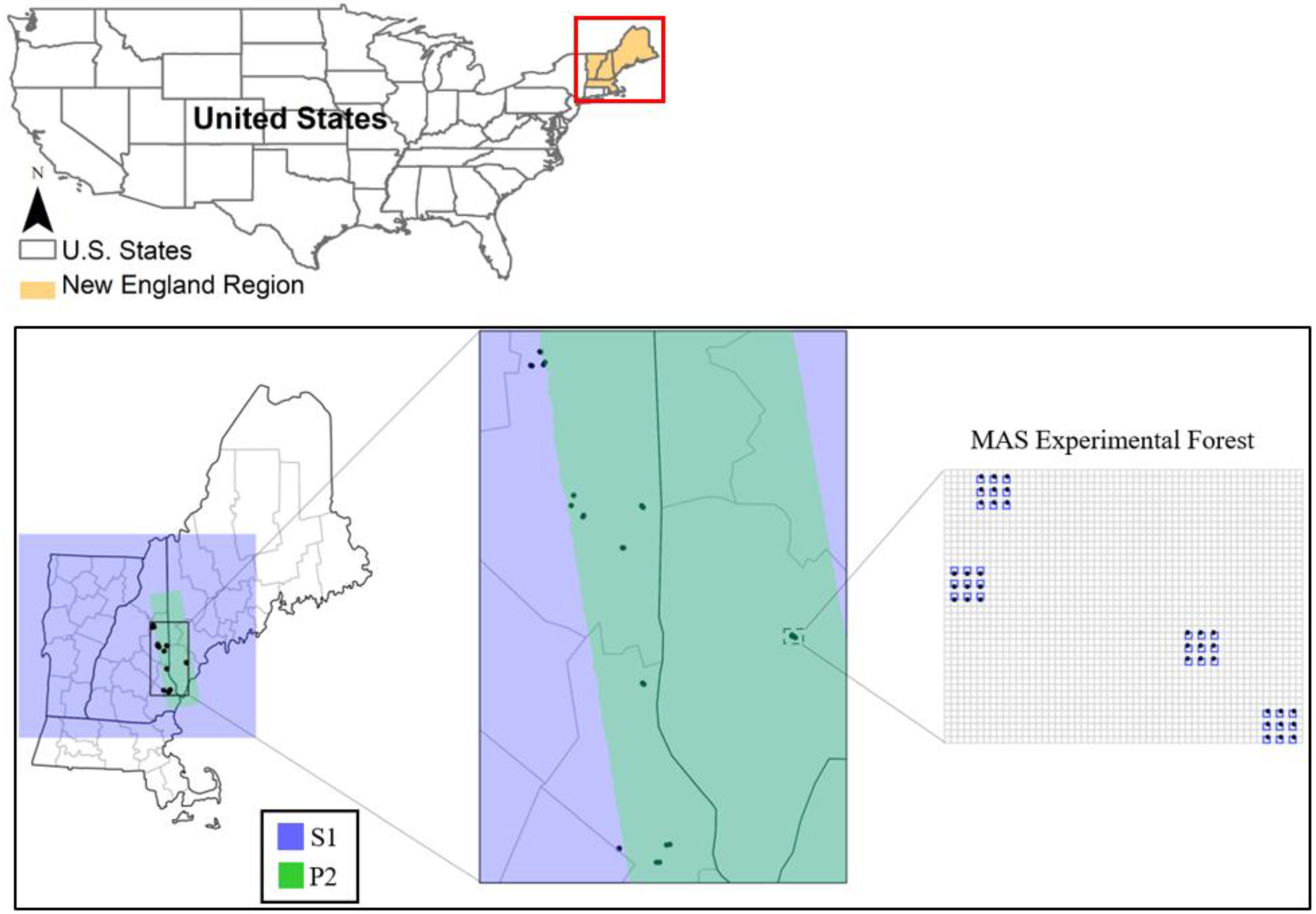
2. Study Area and Data Collection
2.1. AGB Data
2.2. Sentinel-1
2.3. PALSAR-2
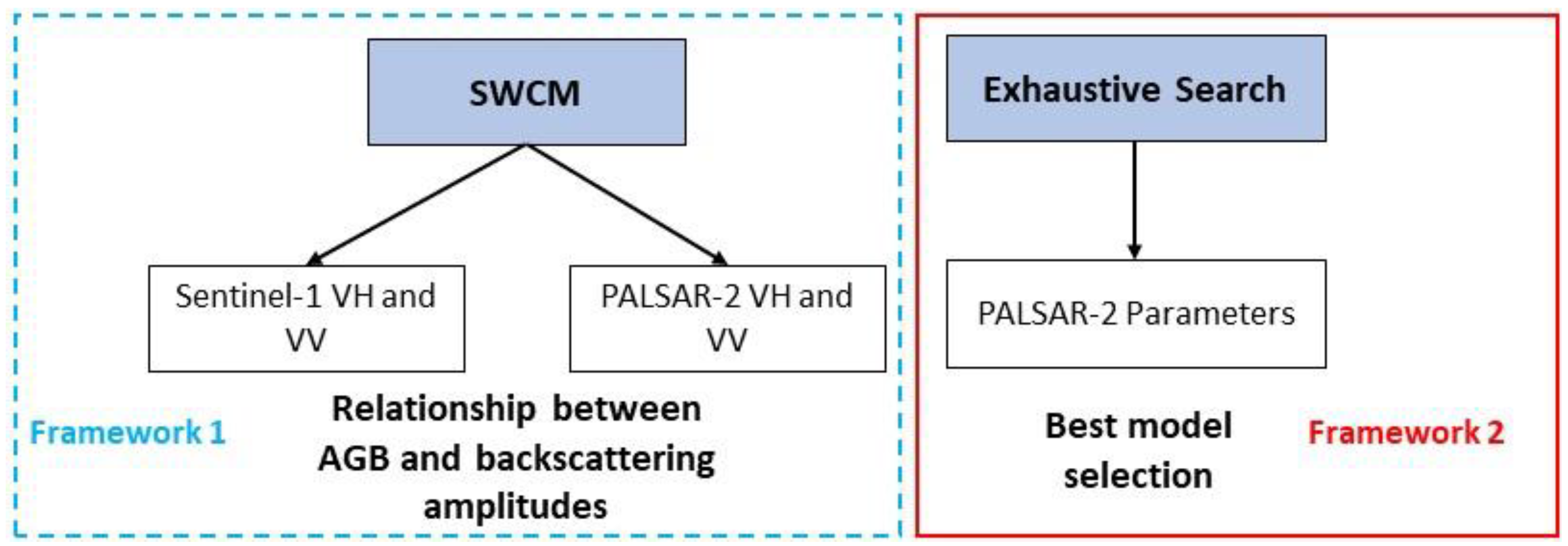
3. Methods
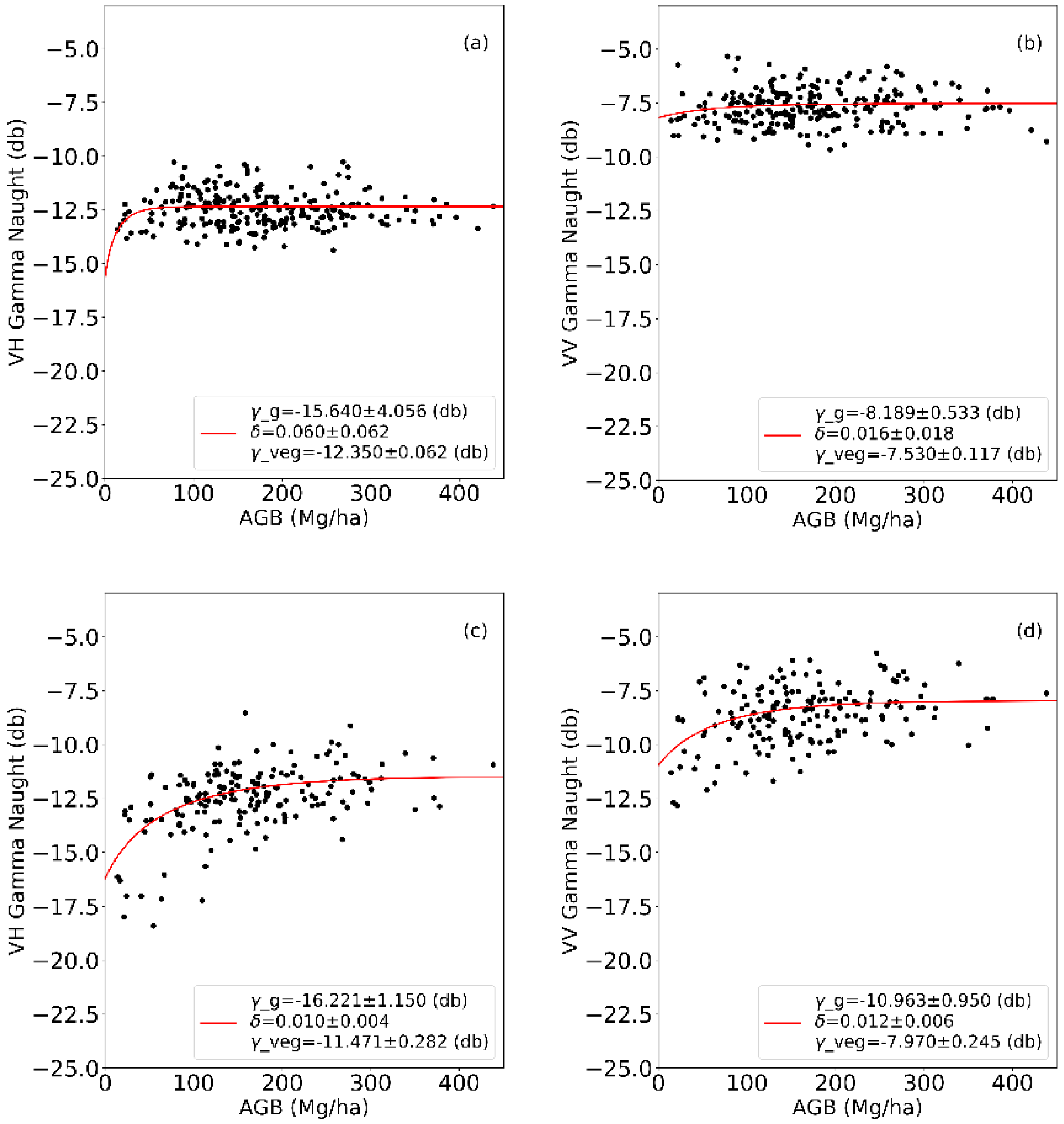
3.1. Simple Water Cloud Model
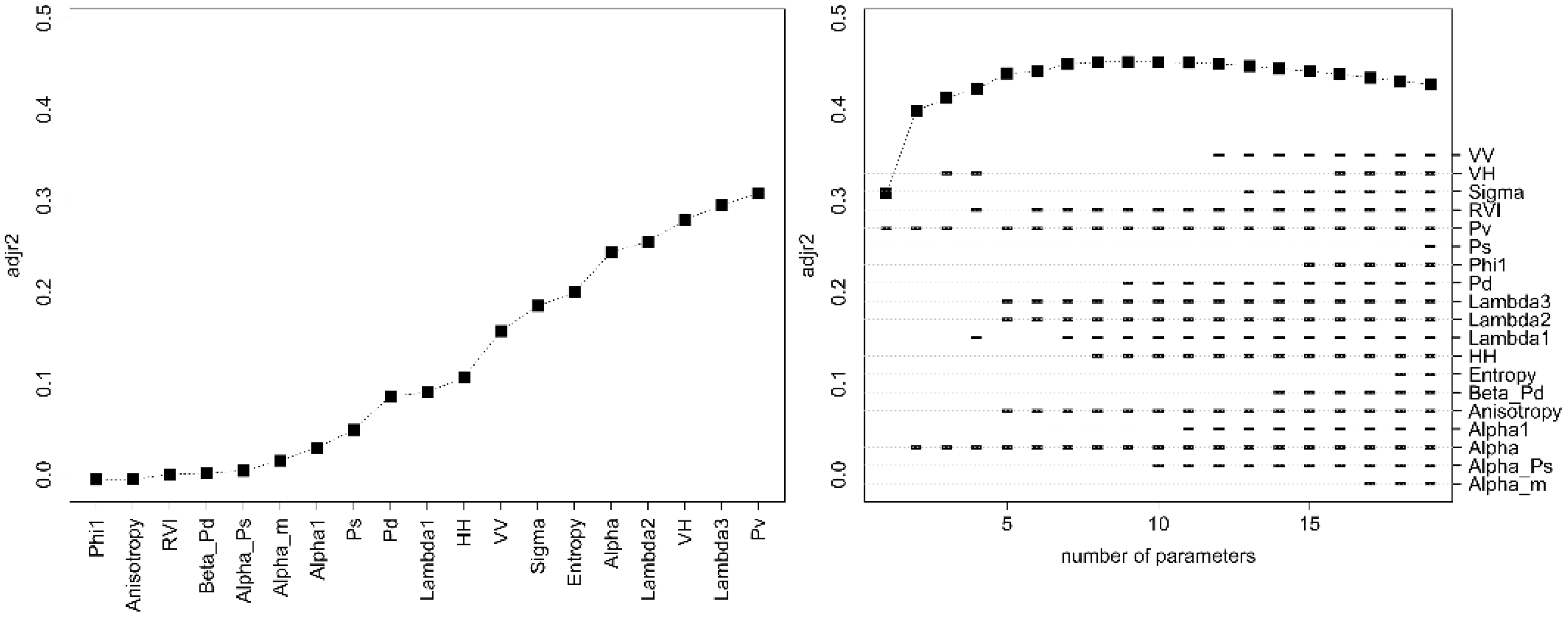
3.2. Exhaustive Search Multiple Linear Regression
4. Results
4.1. Simple Water Cloud Model
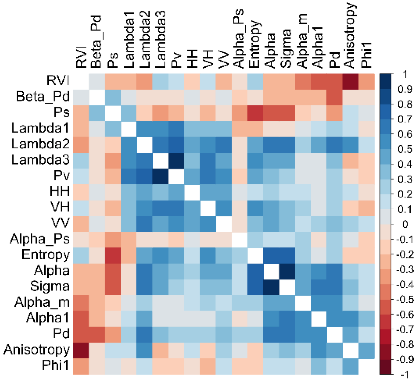
4.2. AGB Estimation from Polarimetric PALSAR-2 Data
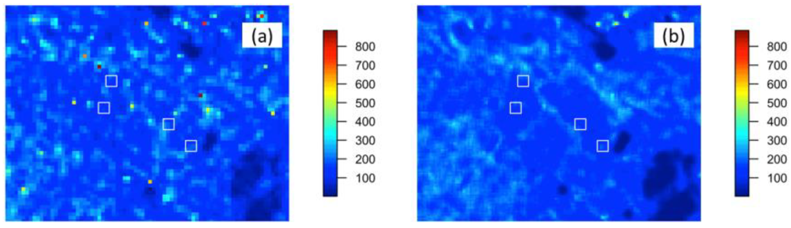
4.3. AGB Estimation from the Single and Multi-Temporal Sentinel-1 Data
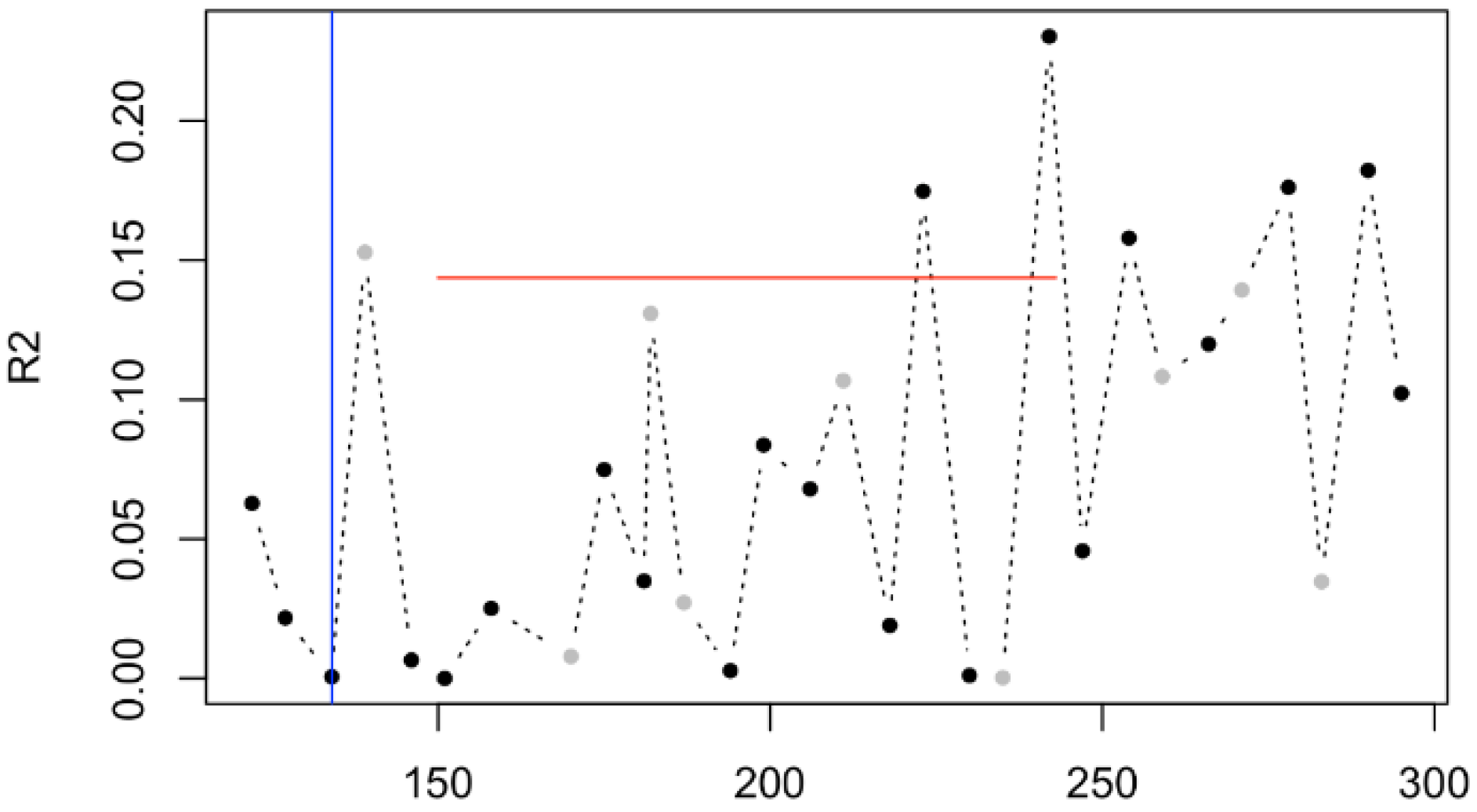
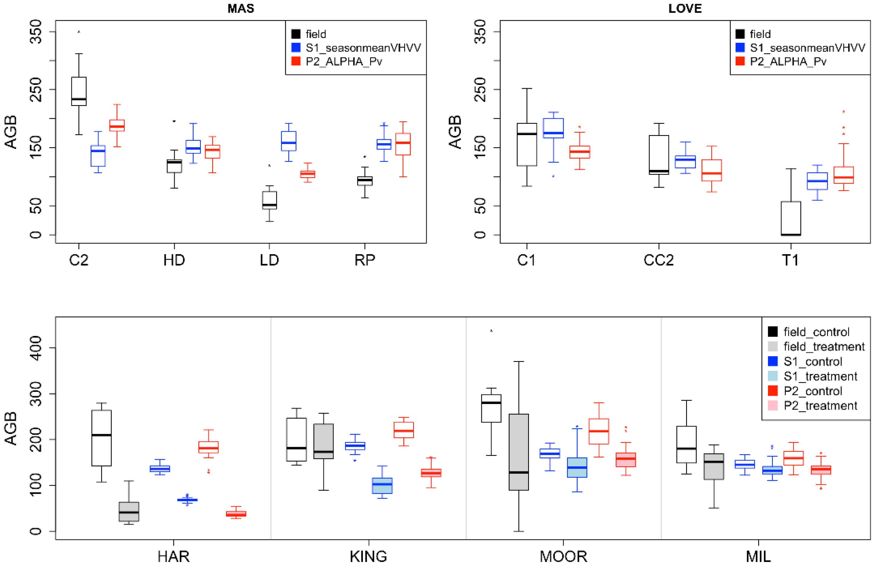
4.4. Relative Biomass Difference Detection at Site Level
5. Discussion
6. Conclusions
Author Contributions
Funding
Conflicts of Interest
References
- Santoro, M.; Cartus, O. Research Pathways of Forest Above-Ground Biomass Estimation Based on SAR Backscatter and Interferometric SAR Observations. Remote Sens. 2018, 10, 608. [Google Scholar] [CrossRef]
- Imhoff, M.L. Radar backscatter and biomass saturation: Ramifications for global biomass inventory. IEEE Trans. Geosci. Remote Sens. 1995, 33, 511–518. [Google Scholar] [CrossRef]
- Le Toan, T.; Beaudoin, A.; Riom, J.; Guyon, D. Relating forest biomass to SAR data. IEEE Trans. Geosci. Remote Sens. 1992, 30, 403–411. [Google Scholar] [CrossRef]
- Sandberg, G.; Ulander, L.M.; Fransson, J.E.S.; Holmgren, J.; Le Toan, T. L-and P-band backscatter intensity for biomass retrieval in hemiboreal forest. Remote Sens. Environ. 2011, 115, 2874–2886. [Google Scholar] [CrossRef]
- Rignot, E.J.; Zimmermann, R.; van Zyl, J.J. Spaceborne applications of P band imaging radars for measuring forest biomass. IEEE Trans. Geosci. Remote Sens. 1995, 33, 1162–1169. [Google Scholar] [CrossRef]
- Santos, J.R.; Freitas, C.C.; Araujo, L.S.; Dutra, L.V.; Mura, J.C.; Gama, F.F.; Soler, L.S.; Sant’Anna, S.J. Airborne P-band SAR applied to the aboveground biomass studies in the Brazilian tropical rainforest. Remote Sens. Environ. 2003, 87, 482–493. [Google Scholar] [CrossRef]
- Rosenqvist, A.; Shimada, M.; Chapman, B.; Freeman, A. The Global Rain Forest Mapping project—A review. Int. J. Remote Sens. 2000, 21, 1375–1387. [Google Scholar] [CrossRef]
- Lucas, R.; Armston, J.; Fairfax, R.; Fensham, R.; Accad, A.; Carreiras, J.; Metcalfe, D. An evaluation of the ALOS PALSAR L-band backscatter—Above ground biomass relationship Queensland, Australia: Impacts of surface moisture condition and vegetation structure. IEEE J. Sel. Top. Appl. Earth Obs. Remote Sens. 2010, 3, 576–593. [Google Scholar] [CrossRef]
- Cartus, O.; Santoro, M.; Kellndorfer, J. Mapping forest aboveground biomass in the Northeastern United States with ALOS PALSAR dual-polarization L-band. Remote Sens. Environ. 2012, 124, 466–478. [Google Scholar] [CrossRef]
- Mermoz, S.; Réjou-Méchain, M.; Villard, L.; Le Toan, T.; Rossi, V.; Gourlet-Fleury, S. Decrease of L-band SAR backscatter with biomass of dense forests. Remote Sens. Environ. 2015, 159, 307–317. [Google Scholar] [CrossRef]
- Peregon, A.; Yamagata, Y. The use of ALOS/PALSAR backscatter to estimate above-ground forest biomass: A case study in Western Siberia. Remote Sens. Environ. 2013, 137, 139–146. [Google Scholar] [CrossRef]
- Saatchi, S.S.; McDonald, K.C. Coherent effects in microwave backscattering models for forest canopies. IEEE Trans. Geosci. Remote Sens. 1997, 35, 1032–1044. [Google Scholar] [CrossRef]
- Ulaby, F.T.; Elachi, C. Radar Polarimetry for Geoscience Applications; Artech House, Inc.: Norwood, MA, USA, 1990. [Google Scholar]
- Bouvet, A.; Mermoz, S.; Le Toan, T.; Villard, L.; Mathieu, R.; Naidoo, L.; Asner, G.P. An above-ground biomass map of African savannahs and woodlands at 25 m resolution derived from ALOS PALSAR. Remote Sens. Environ. 2018, 206, 156–173. [Google Scholar] [CrossRef]
- Ningthoujam, R.K.; Joshi, P.K.; Roy, P.S. Retrieval of forest biomass for tropical deciduous mixed forest using ALOS PALSAR mosaic imagery and field plot data. Int. J. Appl. Earth Obs. Geoinf. 2018, 69, 206–216. [Google Scholar] [CrossRef]
- Mitchard, E.T.; Saatchi, S.S.; Woodhouse, I.H.; Nangendo, G.; Ribeiro, N.S.; Williams, M.; Meir, P. Using satellite radar backscatter to predict above-ground woody biomass: A consistent relationship across four different African landscapes. Geophys. Res. Lett. 2009, 36. [Google Scholar] [CrossRef]
- Hame, T.; Rauste, Y.; Antropov, O.; Ahola, H.A.; Kilpi, J. Improved mapping of tropical forests with optical and SAR imagery, Part II: Above ground biomass estimation. IEEE J. Sel. Top. Appl. Earth Obs. Remote Sens. 2013, 6, 92–101. [Google Scholar] [CrossRef]
- Cloude, S.R.; Pottier, E. A review of target decomposition theorems in radar polarimetry. IEEE Trans. Geosci. Remote Sens. 1996, 34, 498–518. [Google Scholar] [CrossRef]
- Freeman, A.; Durden, S.L. A three-component scattering model for polarimetric SAR data. IEEE Trans. Geosci. Remote Sens. 1998, 36, 963–973. [Google Scholar] [CrossRef]
- Yamaguchi, Y.; Moriyama, T.; Ishido, M.; Yamada, H. Four-component scattering model for polarimetric SAR image decomposition. IEEE Trans. Geosci. Remote Sens. 2005, 43, 1699–1706. [Google Scholar] [CrossRef]
- Touzi, R. Target scattering decomposition in terms of roll-invariant target parameters. IEEE Trans. Geosci. Remote Sens. 2007, 45, 73–84. [Google Scholar] [CrossRef]
- Karam, M.A.; Amar, F.; Fung, A.K.; Mougin, E.; Lopes, A.; Le Vine, D.M.; Beaudoin, A. A microwave polarimetric scattering model for forest canopies based on vector radiative transfer theory. Remote Sens. Environ. 1995, 53, 16–30. [Google Scholar] [CrossRef]
- Antropov, O.; Rauste, Y.; Häme, T.; Praks, J. Polarimetric ALOS PALSAR time series in mapping biomass of boreal forests. Remote Sens. 2017, 9, 999. [Google Scholar] [CrossRef]
- Saatchi, S.S.; Houghton, R.A.; Dos Santos Alvala, R.C.; Soares, J.V.; Yu, Y. Distribution of aboveground live biomass in the Amazon basin. Glob. Chang. Biol. 2007, 13, 816–837. [Google Scholar] [CrossRef]
- Omernik, J.M. Ecoregions of the conterminous United States. Ann. Assoc. Am. Geogr. 1987, 77, 118–125. [Google Scholar] [CrossRef]
- Kershaw, J.A., Jr.; Ducey, M.J.; Beers, T.W.; Husch, B. Forest Mensuration, 5th ed.; Wiley: New York, NY, USA, 2016. [Google Scholar]
- Chojnacky, D.C.; Heath, L.S.; Jenkins, J.C. Updated generalized biomass equations for North American tree species. Forestry 2013, 87, 129–151. [Google Scholar] [CrossRef]
- Hoover, C.M.; Ducey, M.J.; Colter, R.A.; Yamasaki, M. Evaluation of alternative approaches for landscape-scale biomass estimation in a mixed-species northern forest. For. Ecol. Manag. 2018, 409, 552–563. [Google Scholar] [CrossRef]
- Small, D. Flattening gamma: Radiometric terrain correction for SAR imagery. IEEE Trans. Geosci. Remote Sens. 2011, 49, 3081–3093. [Google Scholar] [CrossRef]
- Huang, X.; Wang, J.; Shang, J. Simplified adaptive volume scattering model and scattering analysis of crops over agricultural fields using the RADARSAT-2 polarimetric synthetic aperture radar imagery. J. Appl. Remote Sens. 2015, 9, 096026. [Google Scholar] [CrossRef]
- Huang, X.; Wang, J.; Shang, J.; Liu, J. A Simple Target Scattering Model with Geometric Features on Crop Characterization Using Polsar Data. In Proceedings of the Geoscience and Remote Sensing Symposium (IGARSS), Fort Worth, TX, USA, 23–28 July 2017; pp. 1032–1035. [Google Scholar]
- Attema, E.P.W.; Ulaby, F.T. Vegetation modeled as a water cloud. Radio Sci. 1978, 13, 357–364. [Google Scholar] [CrossRef]
- Thomas Lumley Using Fortran Code by Alan Miller. Leaps: Regression Subset Selection. R Package Version 2.9. Available online: https://cran.r-project.org/web/packages/leaps/index.html (accessed on 7 September 2018).
- R Core Team. R: A Language and Environment for Statistical Computing; R Foundation for Statistical Computing: Vienna, Austria, 2016. [Google Scholar]
- Caicoya, A.T.; Pardini, M.; Hajnsek, I.; Papathanassiou, K. Forest above-ground biomass estimation from vertical reflectivity profiles at L-band. IEEE Geosci. Remote Sens Lett. 2015, 12, 2379–2383. [Google Scholar] [CrossRef]
- Rauste, Y. Multi-temporal JERS SAR data in boreal forest biomass mapping. Remote Sens. Environ. 2005, 97, 263–275. [Google Scholar] [CrossRef]
- Beriaux, E.; Lucau-Danila, C.; Auquiere, E.; Defourny, P. Multiyear independent validation of the water cloud model for retrieving maize leaf area index from SAR time series. Int. J. Remote Sens. 2013, 34, 4156–4181. [Google Scholar] [CrossRef]
- Jiao, X.; McNairn, H.; Shang, J.; Pattey, E.; Liu, J.; Champagne, C. The sensitivity of RADARSAT-2 polarimetric SAR data to corn and soybean leaf area index. Can. J. Remote Sens. 2011, 37, 69–81. [Google Scholar] [CrossRef]
- He, B.; Xing, M.; Bai, X. A synergistic methodology for soil moisture estimation in an alpine prairie using radar and optical satellite data. Remote Sens. 2014, 6, 10966–10985. [Google Scholar] [CrossRef]
- Askne, J.; Santoro, M.; Smith, G.; Fransson, J.E. Multitemporal repeat-pass SAR interferometry of boreal forests. IEEE Trans. Geosci. Remote Sens. 2003, 41, 1540–1550. [Google Scholar] [CrossRef]
- Lee, J.S.; Ainsworth, T.L. The effect of orientation angle compensation on coherency matrix and polarimetric target decompositions. IEEE Trans. Geosci. Remote Sens. 2011, 49, 53–64. [Google Scholar] [CrossRef]
- Kellndorfer, J.M.; Dobson, M.C.; Vona, J.D.; Clutter, M. Toward precision forestry: Plot-level parameter retrieval for slash pine plantations with JPL AIRSAR. IEEE Trans. Geosci. Remote Sens. 2003, 41, 1571–1582. [Google Scholar] [CrossRef]
- Le Toan, T.; Quegan, S.; Davidson, M.W.J.; Balzter, H.; Paillou, P.; Papathanassiou, K.; Ulander, L. The BIOMASS mission: Mapping global forest biomass to better understand the terrestrial carbon cycle. Remote Sens. Environ. 2011, 115, 2850–2860. [Google Scholar] [CrossRef]
- Laurin, G.V.; Balling, J.; Corona, P.; Mattioli, W.; Papale, D.; Puletti, N.; Urban, M. Above-ground biomass prediction by Sentinel-1 multitemporal data in central Italy with integration of ALOS2 and Sentinel-2 data. J. Appl. Remote Sens. 2018, 12, 016008. [Google Scholar] [CrossRef]


| Forest Property Full Name | Forest Short Name | Site | Sample Plots | Description |
|---|---|---|---|---|
| Bartlett Experimental Forest | BAR | 07_C | 9 | White pine-northern hardwood reference |
| 07_T | 9 | White pine-northern hardwood thinning | ||
| 22_C | 9 | Northern hardwood reference | ||
| 22_T | 9 | Northern hardwood thinning | ||
| 35_C | 9 | Northern hardwood reference | ||
| 35_T | 8 | Northern hardwood thinning | ||
| Bear Camp River Property | BEAR | T | 9 | Oak-pine thinning |
| Harmon Preserve | HAR | C | 9 | Pitch pine barrens reference |
| T | 9 | Pitch pine barrens thinned and burned | ||
| Kingman Farm | KING | C1 | 9 | Oak-pine reference |
| T1 | 9 | Oak-pine thinned | ||
| Lord Farm | LORD | LORD | 9 | Oak-pine reference |
| Lovell River | LOVE | C1 | 9 | Oak-pine reference |
| CC2 | 7 | Oak-pine clearcut | ||
| T1 | 6 | Oak-pine thinned | ||
| Massabesic Experimental Forest | MAS | C2 | 9 | White pine-hemlock reference |
| HD | 9 | White pine high-density thinning | ||
| LD | 9 | White pine low-density thinning | ||
| RP | 9 | Red pine plantation | ||
| Mendums’ Pond | MEND | C | 9 | Oak-pine reference |
| T | 9 | Oak-pine thinning | ||
| Jones Forest | MIL | C | 9 | Oak-pine reference |
| T | 9 | Oak-pine thinning | ||
| Moore Fields | MOOR | C1 | 9 | Oak-pine reference |
| T1 | 9 | Oak-pine thinning | ||
| Pine River State Forest | PR | C2 | 9 | White pine reference |
| T1 | 9 | White pine tornado |
| Sensors | Parameters | Description | |
|---|---|---|---|
| Sentinel-1 | VH | VH channel | |
| VV | VV channel | ||
| PALSAR-2 | VH | VH channel | |
| VV | VV channel | ||
| HH | HH channel | ||
| Touzi Decomposition [19] | Lambda 1 | First dominant scattering amplitude | |
| Lambda 2 | Second dominant scattering amplitude | ||
| Lambda 3 | Third dominant scattering amplitude | ||
| Alpha 1 | Dominant polarization angle | ||
| Alpha m | Mean polarization angle | ||
| Phi 1 | Phase difference | ||
| Eigen Decomposition [16] | Entropy | Scattering Entropy | |
| Alpha | Scattering Mechanism | ||
| A | Anisotropy | ||
| SVSM [28] | RVI | Geometric randomness | |
| Sigma | Shape factor | ||
| SAVSM [27] | Ps | Surface Scattering | |
| Pd | Double-bounce scattering | ||
| Pv | Volume scattering | ||
| Beta_Ps | Beta parameter related to surface scattering | ||
| Alpha_Pd | Alpha parameter related to double-bounce | ||
| Model ID | RMSE (Mg/ha) | Parameters |
|---|---|---|
| 1 | 76.72 | Pv |
| 2 | 70.46 | Alpha + Pv |
| 3 | 69.00 | Alpha + Pv + VH |
| 4 | 69.68 | Alpha + Lambda1 + RVI + VH |
| 5 | 68.90 | Alpha + Anisotropy + Lambda2 + Lambda3 + Pv |
© 2018 by the authors. Licensee MDPI, Basel, Switzerland. This article is an open access article distributed under the terms and conditions of the Creative Commons Attribution (CC BY) license (http://creativecommons.org/licenses/by/4.0/).
Share and Cite
Huang, X.; Ziniti, B.; Torbick, N.; Ducey, M.J. Assessment of Forest above Ground Biomass Estimation Using Multi-Temporal C-band Sentinel-1 and Polarimetric L-band PALSAR-2 Data. Remote Sens. 2018, 10, 1424. https://doi.org/10.3390/rs10091424
Huang X, Ziniti B, Torbick N, Ducey MJ. Assessment of Forest above Ground Biomass Estimation Using Multi-Temporal C-band Sentinel-1 and Polarimetric L-band PALSAR-2 Data. Remote Sensing. 2018; 10(9):1424. https://doi.org/10.3390/rs10091424
Chicago/Turabian StyleHuang, Xiaodong, Beth Ziniti, Nathan Torbick, and Mark J. Ducey. 2018. "Assessment of Forest above Ground Biomass Estimation Using Multi-Temporal C-band Sentinel-1 and Polarimetric L-band PALSAR-2 Data" Remote Sensing 10, no. 9: 1424. https://doi.org/10.3390/rs10091424
APA StyleHuang, X., Ziniti, B., Torbick, N., & Ducey, M. J. (2018). Assessment of Forest above Ground Biomass Estimation Using Multi-Temporal C-band Sentinel-1 and Polarimetric L-band PALSAR-2 Data. Remote Sensing, 10(9), 1424. https://doi.org/10.3390/rs10091424