Next Article in Journal
3D Point Cloud Semantic Modelling: Integrated Framework for Indoor Spaces and Furniture
Previous Article in Journal
Mapping Population Distribution from High Resolution Remotely Sensed Imagery in a Data Poor Setting
 
 
Reply published on 8 September 2018, see Remote Sens. 2018, 10(9), 1432.
Comment

Comment on Tompalski et al. Combining Multi-Date Airborne Laser Scanning and Digital Aerial Photogrammetric Data for Forest Growth and Yield Modelling. Remote Sens. 2018, 10, 347

Natural Resources Institute Finland (Luke), Bioeconomy and Environment Unit, Yliopistokatu 6, FI-80100 Joensuu, Finland
Remote Sens. 2018, 10(9), 1411; https://doi.org/10.3390/rs10091411
Submission received: 4 July 2018 / Accepted: 24 August 2018 / Published: 5 September 2018

Abstract

:
Tompalski et al. (2018) propose “template matching” as a (required) intermediate step to use remote sensing-based predictions of forest attributes as inputs of the Growth and Yield Projection System (GYPSY) for the simulations of forest stand dynamics in Alberta, Canada. Yet, the feasibility of the approach can be criticized for many points that call for experimental verification. The approach cannot be fully replicated based on the description of the paper. Nevertheless, an experimental implementation with synthetic data indicates that the quality of the projections may vary considerably depending on parameter assumptions for the templates, and the projections may include discontinuities between the observed and projected forest attributes. The approach is poorly motivated given that the effects described above are largely avoidable, if the underlying GYPSY models are run without the template matching step. The R-codes used for the analyses are provided as supplementary data for an interested reader wishing to evaluate the conclusions made above. A semantic analysis indicates further problems with multi-date data on a wall-to-wall grid. The projections obtained by template matching should be exposed to criticism for their realism and benchmarked against other approaches prior to using template matching as proposed by Tompalski et al.

1. Introduction

Tompalski et al. [1] propose “template matching” as an intermediate step from remote sensing-based predictions to forest growth and yield projections. In the proposed approach, a set of forest attributes (top height, density, basal area, total volume in [1]) are predicted for selected spatial units (sample plots or 20 × 20 m2 grid cells in [1]) based on remotely sensed data (airborne laser scanning and digital aerial photogrammetric data in [1]). The subject stands are assumed to be covered by existing inventory data including age and species information. In the template matching, existing growth models are first run with all possible combinations of their input parameters to generate a database of growth trajectories (=templates). Among the templates, the ones that best agree with the aforementioned forest attribute predictions for the given age and species are selected as the trajectories used for growth and yield projections (=matching). The idea of the template matching approach is condensed to Figure 1a from the original, more detailed illustration [1] (Figure 4).
Tompalski et al. vaguely motivate the need to use the template matching approach by discrepancy between remotely sensed outputs and growth model inputs, especially in the case of grid cells [1] (Section 1). However, reasoning the approach on such a basis can be questioned, because not even conventional inventories provide a forest attribute combination that is exactly the same as required by growth and yield models. Instead, decades-old growth and yield modeling systems are composed of model chains to derive the required inputs from the limited measurements [2,3,4], and the same model chains can be readily applied to grid-based inventory data without specific attention on the growth and yield modeling methodology, as demonstrated in plantations [5] and semi-natural forests [6,7].
Instead of clearly identifiable benefits of including template matching as an intermediate step for remote sensing based future projections, a cursory glance at the proposed approach does raise a few caveats. To apply the template matching over a wall-to-wall forest inventory grid and multiple time points, Tompalski et al. present prediction models [1] (Table 4) that were fit independently for each considered forest attribute and time points T1 and T2. It is worthwhile to note that the training data covering both T1 and T2 were repeated measurements of the same plots. Consequently, the residual errors between the stand attributes and time points cannot be considered independent of each other, which is against the assumptions of ordinary least squares regression applied for model fitting [1]. The following practical considerations of combining the proposed template matching approach with the independent modelling of the different forest attributes at the different time points should subsequently be made:
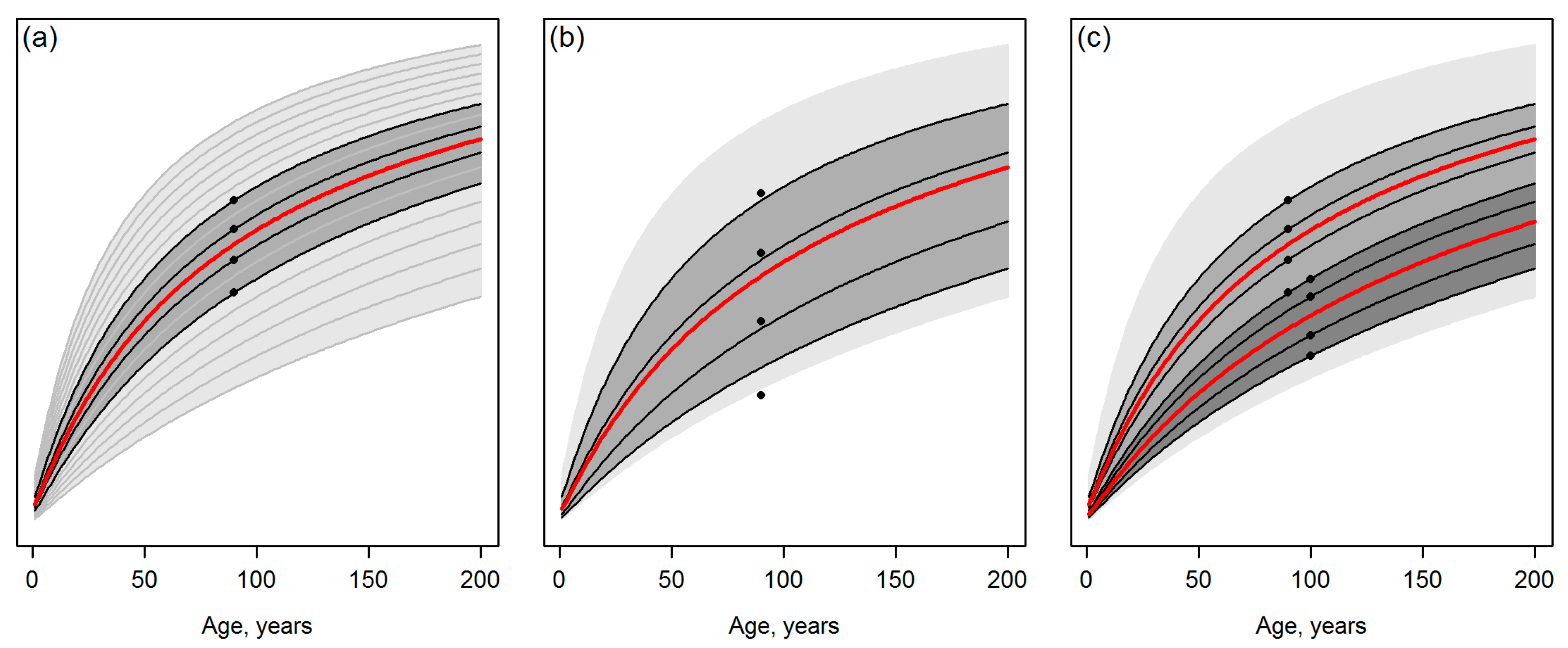
  • Assume that Figure 1a represents an ideal case with error-free observations, whereas predicting the attributes of interest independently of each other for a grid cell hinders the curve matching as illustrated in Figure 1b. Tompalski et al. [1] do conclude that “the accuracy of curve matching was dependent on the ABA (area-based approach) prediction error”. However, what are the implications of a lower “accuracy of curve matching”? What is the sensitivity of the approach to produce such a severe incompatibility (e.g., [2] (Chapter 15)) between stand attributes or their future projections that causes problems for the further use of this information? Are there interactions in this sense between the composition of the observations and the template database (for example, what if observations or predictions are located on borders or slightly outside of the template space such as the lowest observation of Figure 1b)?
  • Assume that multi-date data are available (Figure 1c) and observations or predictions for T2 systematically suggest a slower future development of the stand, compared to single-date observations or predictions for T1. Note that even if the training data for model fitting were filtered for recorded disturbances between the two time steps (as in Tompalski et al. [1]), situations corresponding to Figure 1c could occur due to artifacts in the remotely sensed data and ignoring the dependencies between T1 and T2 in the prediction models. Applying the workflow of Tompalski et al. [1] to wall-to-wall forest inventory grid data from multiple dates would thus produce situations that resemble real-world disturbances in the forest (cf. Figure 1c), but it is unclear if and how the underlying growth and yield modelling system logic can manage such situations.
  • Overall, how well-reasoned is that with multi-date data, “the weighted means were calculated separately for each data set, and then averaged” [1] (Section 3.3), i.e., the observations for T1 and T2 were considered with an equal weight, even if the latter represent data acquired later and should therefore have a closer temporal match with the present forest state?
The text above suggests that even if the template matching approach is based on existing growth models, the selecting and averaging process involved probably yields final growth trajectories that may have considerably different properties from those included in the database. Therefore, even if the underlying growth models were adequately evaluated for their realism (cf. [2] (Chapter 15); [3] (Chapter 18); [8,9]), a similar model criticism should be applied to the outputs of the template matching. The evaluation should probably account for potential interactions between the parameters of the underlying growth models and random prediction errors in the forest attributes used as inputs of the template matching.
To verify and quantify the points listed above, I simulated the template matching approach [1] with synthetic data. In the comment below, I particularly focus on effects of parameter choices on the subsequent template generation and matching. Since a number of assumptions was made, the experimental implementation is described in detail and provided as R-code [10] in files mentioned in the sub-titles of Section 2. I discuss the results from model criticism and benchmarking points of view.

2. Experimental Implementation

2.1. The Growth and Yield Projection System (GYPSY) Models (gypsy_models.R)

The Growth and Yield Projection System (GYPSY) underlying the template matching approach was implemented as closely as possible to correspond with Tompalski et al. [1] following the model documentation [11]. However, neither Tompalski et al. [1] nor the model documentation provide guidance on many choices regarding possible parameterizations. First, both non-spatial and spatial versions of the GYPSY models are available [11], but Tompalski et al. [1] do not indicate which one they used. The choice between a spatial or non-spatial framework could be expected to result in fundamental differences in the required parameterization, because “spatial” models normally involve spatially explicit competition indices based on tree-to-tree distances or similar measures (for hints on required computations, see e.g., [12,13] or [3] (Chapter 9)). However, a more thorough look at the models [11] indicates that this is not the case with GYPSY. Compared to the non-spatial version, the “spatial” GYPSY only includes an additional percent stocking component, which is predicted from tree density using additional models provided [11]. One cannot therefore expect that the non-spatial and spatial GYPSY projections would fundamentally differ. However, because the non-spatial models had considerable simpler forms, the non-spatial version of GYPSY [11] was selected for the analyses below.
GYPSY is implemented as a collection of sub-models for the different attributes [11]. The sub-models differ by parameters and even model forms depending on species (group). I derived the projections separately for species groups of Aspen, Pine, Black spruce and White spruce, which correspond to those used by Tompalski et al. [1]. Regardless of species, the models of interest for this exercise take the following arguments:
Htop = f(SI, age),
N = f(SDFsp, SI),
BAINC = f(age, SI, Nini, SC, BA), and
Tvol = f(BA, Htop),
where Htop is the average height of the 100 largest DBH trees per ha (m), SI is the site index (m), age is the stand age, N is the density (stems/ha) of the subject species, SDF is a species-specific stand-density factor defined as N at 50 years of age, BAINC is the annual basal area increment for the subject species (m2/ha/year), Nini is the initial density at the age of zero, SC is the current species composition (Nspecies/Nall), BA is the current basal area (m2/ha) for the subject species, and Tvol is the gross total volume (m3/ha) “of the subject species at the 0/0 utilization standard” [11]. The models presented in Equations (1)–(4) correspond to those numbered by 4, 5, 6 and 10, respectively, in the GYPSY documentation [11], with naming conventions of the variables somewhat simplified for the present purpose. In addition, I have made the following simplifications when implementing the models:
  • Above, the definition of “age” varies between models and tree species (groups): it is either total age (years since the point of germination) or breast height age (age at the height of 1.3 m above ground). Consequently, SI is the top height corresponding to the age definition that varies between the models and species. For my exercises, I assumed that all age and SI values inputted corresponded to the breast height age. Where necessary, I converted the breast height age to total age using average conversion factors [11] (p. 5). However, I did not convert SI, i.e., SI values between Equation (1) and the other models are not consistent regarding the definition, which causes a leveling difference with a magnitude that probably could be assessed by applying exact conversions [11] (Appendix A). This is further explored below.
  • GYPSY provides a possibility to simulate growth and yield for both pure and mixed stands [11]. Tompalski et al. [1] do not indicate whether their stands were considered to be pure or mixtures of species. For the simulations below, I assumed pure stands. This choice affected the parameterization of Equations (1)–(4) as follows: The SC component of the BAINC model (Equation (3)) was always fixed to 1. The GYPSY models of BAINC additionally include term k, which is computed for the Aspen and Pine species as a transformation of the other model parameters. However, for the two Spruce species, the term k included the SDFs for each of the other three species. In the stands simulated here, where no other species occurred, the term k of the Spruce species received a value of zero.
Due to the missing details, it was additionally found impossible to guess the required parameterization for N (Equation (2)). The model required the species-specific SDF as a key input parameter and neither the model documentation [11] nor Tompalski et al. [1] provide any information on an allowable range for this parameter. For this reason, implementing Equation (2) was entirely omitted, i.e., the template matching below was based on three models (Htop, BAINC, and Tvol to produce the top height, basal area and total volume, respectively), which should ease the matching task (cf. Section 2.3) compared to Tompalski et al. [1] who used all four attributes. However, none of the above simplifications is expected to affect general conclusions made based on the simulations, at least when the growth trajectories are examined species at a time and no between-species comparisons are made.

2.2. Template Database (generate_templates.R)

The following instructions [1] (Section 3.2) were followed to generate the template database (grey lines of the schematic Figure 1a):
Following the approach of Tompalski et al. [21], we used the simulator to create a database of yield curve templates based on all possible input combinations (e.g., every combination of species groups, top height, total age, density, and basal area). The database represented all possible stand conditions in the study area and was based on the range of stand attributes in the existing forest inventory. The yield curves were generated for the four specified species groups, from 1 to 200 years, by 1 year increments. An individual yield curve template consisted of four sequences of values representing top height, basal area, volume, and stem density, between 1 and 200 years, and being estimated by the simulator based on species group, top height, total age, and basal area.
Juxtaposing the above instructions with the GYPSY models (Equations (1)–(4)) provides a clear idea of how the models should be parameterized for age (a sequence of values from 1 to 200 with an interval of 1). The above instructions provide no ideas on allowable ranges for any other required input parameters of Equations (1)–(4) and this information cannot be found from either Tompalski et al. [1] or the model documentation [11]. Therefore, the ranges for the remaining parameter values were obtained from various different sources as described below:
  • Site index (SI) as a sequence of values from 5 to 30 m with an interval of 1 m. The range was obtained as the one that included all observations for the species considered here, according to a graphical interpretation of the GYPSY Validation Summary report [14] (Figures 1 and 6).
  • The initial density at the age of zero (Nini) as two alternative sequences: (1) from 700 to 2700 stems/ha with an interval of 100 stems/ha or (2) from 700 to 6700 stems/ha with an interval of 1000 stems/ha. The values above are derived from common tree spacing used for artificial regeneration in Alberta [15]. Even though a fixed density such as 2400 stems/ha could be assumed as the most typical tree planting density, the reference cited above also mentions natural regeneration as a possible method for Alberta [15], which probably results to more variations of Nini obviously impacting the GYPSY projections [11]. When neither regeneration type could be assumed, two alternative sequences of Nini values were used to derive two distinct template databases. The motivation was to assess how the alternative parameter ranges affect the growth trajectories and, subsequently, how they potentially propagate the template generation and matching.
  • The GYPSY model documentation indicates that the BAINC model (Equation (3)) could be run with or without knowledge on the current basal area [11]. How to do it is, however, not trivial based on the model documentation [11] and Tompalski et al. [1] do not mention if the basal area predictions were explicitly used as the current basal area in the models. In the analyses below, a single basal area sequence corresponding to the age sequence was generated by running the BAINC model (Equation (3)) as follows. First, the BAINC model was run with age = 1, current basal area set to 0, and other parameters as each of the possible combinations of the sequences described above. Then, the obtained BAINC was added to the previous basal area and, incrementing the basal area similarly for each age value, the iteration was continued until a single basal area sequence was obtained for each of the parameter combinations above. The sequences generated this way are abbreviated as G to differentiate from BA used in Equations (3) and (4). To obtain Tvol (Equation (4)), G was used together with Htop obtained from Equation (1) as parameters of Equation (4).

2.3. Template Matching (matching.R)

The two key statements [1] (Section 3.3) were used as instructions to implement the template matching to project the attributes based on observations of a single point in time:
First, candidate curves were selected from the database, based on stand age, species group and the minimal difference between the stand attribute and a value of a yield curve.
and
the final yield curve was derived by calculating a weighted mean of the candidate curves, with the percent of explained variance in the ABA model used as a weight.
Test data are thus required to test the template matching according to the first statement. A test data set was generated by taking the mean species-specific stand age [1] (Table 1) and mean top height, basal area, and total volume of the predictions at T1 [1] (Table 2) and combining these attributes as one observation per species (Table 1). It should be noted that attribute combinations shown in Table 1 might not occur in real forests. However, because these values are the means of the data used to fit the prediction models [1] (Table 4) and the different attributes were modeled independently by Tompalski et al. [1], it is reasonable to assume that combinations presented by Table 1 could occur among their predicted forest attributes.
The test data (Table 1) were matched with the template databases generated above. According to the second statement, I considered weighting the model predictions for the template matching by the variance the models explained. However, because of the small differences in the adjusted coefficients of determination for the attributes considered (the R2 values for the T1 models in [1] (Table 4) were 0.76, 0.71, and 0.78 for the top height, basal area, and total volume, respectively), I found more straightforward for this exercise not to weight the attributes.

2.4. Evaluation (draw_fig2.R & draw_fig3.R)

The results of the experimental implementation are presented below for Aspen, which was the most common species in the plot data of Tompalski et al. [1] (Table 2). The emphasis below is on a graphical interpretation of Figure 2 and Figure 3, which can be reproduced with varying assumptions by running the earlier R scripts sequentially before those mentioned in the sub-title.
Figure 2 presents the candidate templates and the matching result based on using the Nini parameter values (Section 2.2) of either 700 to 2700 stems/ha with an interval of 100 stems/ha (Figure 2a–c) or 700 to 6700 stems/ha with an interval of 1000 stems/ha (Figure 2d–f). A glance at the Figure 2 suggests that the sparsity of the template database varies considerably depending on this choice. The height templates are the same in both Figure 2a,d, because no other parameters than age and SI were included in the respective model (Equation (1)). Yet, the difference between the number of possible templates for this attribute vs basal area and total volume can clearly be observed. Further, the number of templates and their spread and density vary for the latter attributes depending on the Nini parameter range applied (compare Figure 2b–c to Figure 2e–f).
The curves matched with the field observations and the averaged curves are shown in Figure 2, but Figure 3 can be used for an easier comparison between the development trajectories, which are clearly different for the two distinct template databases. The development trajectories of each attribute are specifically noted to include a discontinuity between the observation and the growth curve, which originates from the averaging between the initial candidate curves and varies between attributes depending on the match of the observations and the template curves. A numeric characterization and comparison of the development trajectories is omitted due to known inconsistency of the site index definition between Equations (1), (3) and (4) (Section 2.1), for example.
For benchmarking purposes, Figure 3 also presents projections that can be directly obtained from the GYPSY models, i.e., parameterizing Equations (1), (3) and (4) by the same inputs as above, but without the template matching step. To obtain the top height projection (Figure 3a), Equation (1) was used with the same SI value as above. To obtain the basal area projection(s) (Figure 3b), Equation (3) was used with the same SI as above, basal area of 32.3 m2/ha for the initial age of 81 years (Table 1), and Nini of 700 and 6700 stems/ha, i.e., the range for these values assumed above. To obtain the total volume projection (Figure 3c), Equation (4) was used with the top height and basal area sequences obtained from the previous steps. Notably, assuming similar inputs as were available for the template matching, the direct use of the GYPSY models provided projections that were less affected by the range of the Nini values, included no similar discontinuities and, overall, resembled the attribute-specific candidate curves of the template matching more than the averaged ones. One could consider the starting point of the volume projection to be disconnected from the volume observation. However, the use of the lower value can be motivated by consistency from the point of view of the applied growth and yield modeling system: the volume estimate is produced by Equation (4) and it is therefore compatible with other attributes of the system.

3. Discussion

3.1. Implications of the Results from the Experimental Implementation

It is acknowledged that the simulation described above may suffer from the number of simplifications that had to be made when implementing the GYPSY models and the subsequent template matching due to the lack of essential details on the required parameters (cf. Section 2). Given that R-codes used for deriving the results are included as supplementary data, an interested reader may re-parameterize the template matching by better knowledge on applicable parameter ranges or test the sensitivity of the assumptions made. Yet, I believe that the conclusions made below are valid irrespective of nuances of the parameterization and rather relate to the feasibility of the template matching approach itself.
The lack of details given by Tompalski et al. [1] for the model parameterization could originate from the use of interfaces with fixed parameter values to generate curve templates. Whatever the reason, the implementations of Tompalski et al. [1] are unlikely based on a full understanding of the underlying models, which is underlined by few instances in the paper: First, if the authors had carried out similar exploratory analysis as above, they would unlikely assume “that errors introduced by GYPSY’s internal sub-models are equal for each projection and consequently we did not account for them in our study” [1] (Section 3.2). On this point, look at Equations (1)–(4) and especially Equation (4): using the outputs of earlier models as inputs of following ones cannot result but a significant correlation of the errors between the sub-models. Second, it is unclear if the authors carried out the template matching step using the current basal area as a parameter of Equation (3) and the top height and basal area from the GYPSY’s internal sub-models as parameters of Equation (4), which would both have improved the consistency of the matched attributes and the templates from the growth and yield system point of view. Third, based on the statement “Following the approach of Tompalski et al. [21]…” [1] (Section 3.2), a reader could expect the earlier publications to provide hints for the multiple parameter choices yearned for above (Section 2). The same reader might be disappointed, however, to find out that the underlying growth model of that paper was different and the description was thus not helpful for implementations where GYPSY was used as the underlying growth and yield projection system.
Tompalski et al. [1] validated their future projections essentially by comparing both the observed and predicted forest attributes projected to 80 years of age. Such a choice can be criticized: if the predictions and validation data are blindly run through the same (here, template matching) process and only the resulting numbers are compared, there is a fair chance to miss semantic or logical problems potentially affecting the projections based on different input data the same way. Also, given that no validation data with a longer time lag between the observations and projections existed, the assessment of the template matching method would clearly have benefitted from a qualitative analysis of the projections relative to the properties of the underlying models and data. According to such an analysis with artificial data as above, the results and discussion of Tompalski et al. [1] lack for the following remarks, in addition to those pointed out in Section 1 of this comment:
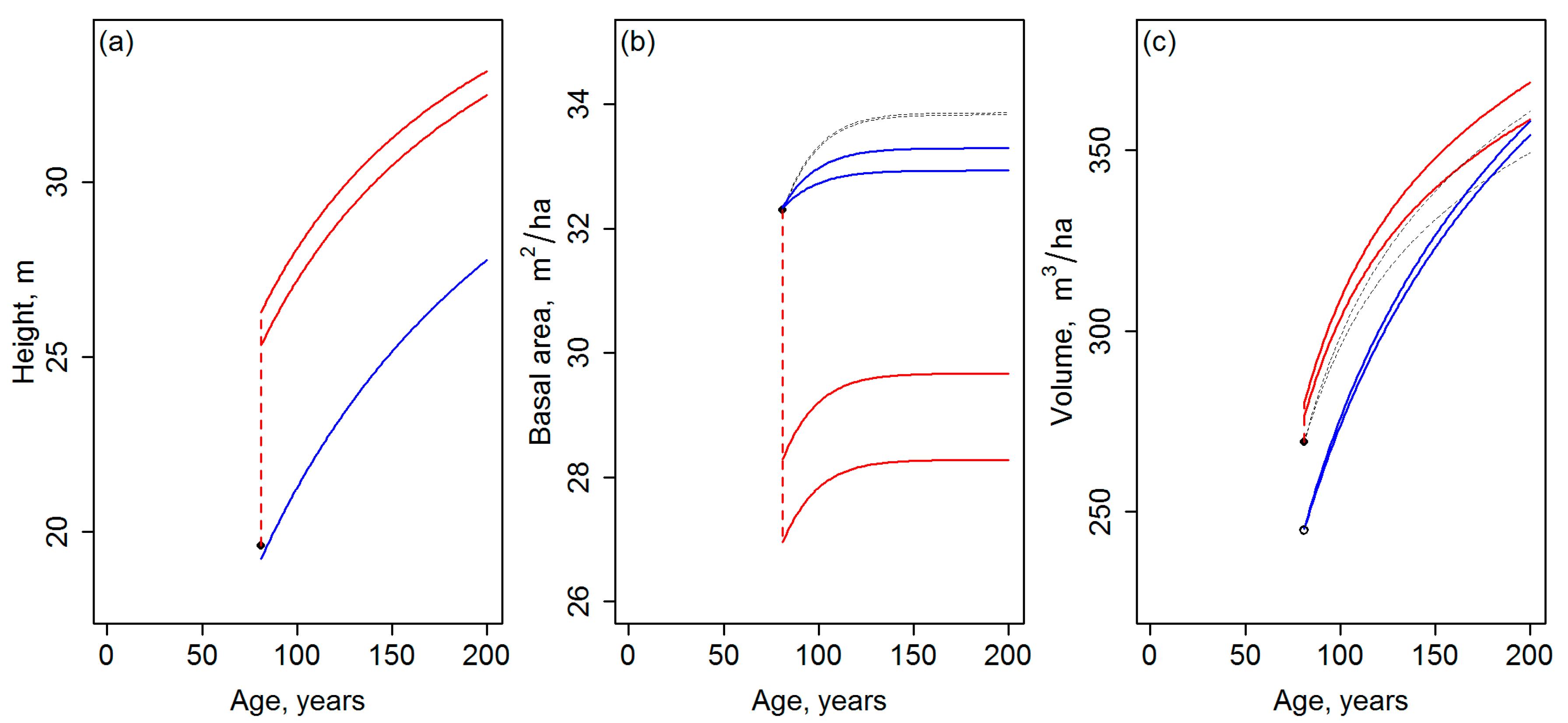
  • The results of the template matching are very sensitive to the assumptions made when generating the template database, for which reason the results should be presented as a function of the applied parameters. With the GYPSY models, especially assumptions on the initial tree planting densities (Nini) had a considerable effect on the final development trajectories obtained. The template matching could even produce trajectories with different site indices, when carried out with template databases based on different assumptions on Nini. Whether the driver for the future development is either different planting density or productivity (site index) affects the future growth and yield estimates drastically, especially if the simulations are continued beyond the current rotation.
  • Template matching may inherently produce discontinuities between the current state of the forest and its projected future state. Note that in Figure 2 and Figure 3, the discontinuities are probably magnified, because the site index differing between Equations (1) and (2) by its definition was not standardized (Section 2.1). Nevertheless, it is difficult to argue against the risk for the discontinuities, considering that observations or predictions are matched with the templates independently (cf. Figure 1). Tompalski et al. [1] do not seem to identify this problem, but to confirm the usability of the projections, those should be exposed to “model criticism and benchmarking” [2] (Chapter 15), with emphases on verifying the biological realism and compatibility of the resulting attributes (see also [3,8,9] (Chapter 18)) with respect to above.
The use of the template matching approach is overall poorly reasoned given the fact that the underlying GYPSY models could be used directly avoiding the problems described above. The direct use of the GYPSY models provides no discontinuities between current and future forest attributes and is much less affected by assumptions related to initial density (Figure 3). To use the GYPSY models as described above requires SI and BA as inputs for the model chain (Equations (1)–(4)). Also, this approach should thus be tested in a real prediction situation, because especially SI is a difficult parameter for remote sensing based inventories. Even so, it is not intuitive to assume that the combination of the two attributes (SI and BA) required to run the GYPSY models was predicted less accurately than the combination of four attributes (H, BA, V, and stand density) required by the template matching [1]. In fact, the availability of SI would also allow the modelling of the stem number: SDFsp is the only additional parameter for the related model (Equation (2)) and it could be possibly obtained as a table value from a stand register, for example, since it affects the projections by GYPSY much less than those involving the template matching step (Figure 3). Making the same assumptions as Tompalski et al. [1] on the availability of data (error-free species and age + the estimates of the forest attributes), it is not infeasible to assume that a similar or better performance was obtained by using the GYPSY models directly with the predicted SI and BA.

3.2. Further Aspects Not Covered by Numeric Examples

The results above describe a simulation based on only one artificial observation. It is acknowledged that a much more complex analysis would be needed to fully conclude on operating the template matching with a wall-to-wall forest inventory grid for multiple time points, i.e., the full framing of Tompalski et al. [1].
To assess template matching with multi-temporal data, one could simply re-run the analyses replacing the values for T1 (Table 1) in the R-codes by those presented for T2 [1] (Tables 1 and 2). The only additional step is that “the weighted means were calculated separately for each data set, and then averaged” [1] (Section 3.3). However, the main implication of this step would be to answer to the question given as the third bullet point of Section 1 in this comment. Treating T1 and T2 equally or setting more weight to the older data could overall be motivated by a higher reliability of these data [16,17], but no such conclusions can be unambiguously made based on the accuracy figures [1] (Table 4, Figure 4). When applied with equal weights, the multi-date data cannot be theoretically expected but to widen the template space from which the final growth trajectory is chosen—i.e., result to a similar decrement of accuracy as erroneous predictions of single point in time (Figure 1). This observation may explain why the authors find so little value of including data from two time points and it would be interesting to see if the same conclusion was made based on the same data, if more delicate weighting [16,17] and selection of the uncertainty metrics according to the prediction framework and available data [16,17,18] were applied. Such a benchmarking could possibly be built upon existing R packages; e.g., [19].
Tompalski et al. [1] (Section 4.4) present wall-to-wall projections, where the template matching approach is applied to a landscape composed of individual grid cells, but do not validate the quality of these results. It is acknowledged that the random errors originating in the predictions of forest attributes for the grid cells and non-random errors related to operating the template matching approach might either cumulate or cancel out each other, and the actual effects should be examined in a further analysis. A short comment on why the analyses above were not extended to the wall-to-wall case is made (see Appendix A). A reader questioning if the problems with compatibility and realism actually occurred in the data of Tompalski et al. might also wish to look at Plot 58 [1] (Figure 5) from the point of view of a biologically credible reasoning for the development of basal area and stem number as predicted for T1 and T2. Based on the above, further analyses are suggested to verify the realism of the template matching for the forest inventory grid.
Remote sensing based forest growth and yield modeling still needs improvements, but the rationale for new, data-driven methods should be grounded on expertise of the growth and yield modeling research dating back decades [2,3,4,8,9]. Even if the GYPSY models were as such found adequate for the projections, involving expertise from both the disciplines mentioned above in an analysis of the existing model forms might reveal possibilities to enhance growth predictions by remote sensing while still retaining coherent information from the growth and yield modeling point of view. For example, if one inferred the percent stocking component for the “spatial” GYPSY models (Section 2) using observed variation among neighboring grid cells instead of using GYPSY sub-models, that would readily allow truly spatial simulations and accounting for within-stand variation in the growth projections that is mentioned as a desirable goal by Tompalski et al. [1].
I find it important to mention that the confusion related to the methods [1] was already pointed out—first in an anonymous review statement and then in personal communication with the authors and the Editorial Board of the Forest Section of Remote Sensing. Publishing the paper in its current form is in a strong controversy with my review statement, which was obviously not presented in a similar extent as above, but most likely in a sufficient detail. Discouraged by this experience and to avoid further waste of time in the future, I wish that the Editors better aligned the editorial policy for papers with a scope clearly exceeding ‘pure’ remote sensing. I encourage the Editors to share my review statement and point out the aspects that needed clarification with respect to above; or clearly indicate if papers submitted to Remote Sensing are expected to be reviewed only per technical and language aspects, while forest growth and yield researchers wishing to deliver and receive detailed feedback and reviewer scrutiny should focus on other forums for their work.

4. Conclusions

The template matching approach cannot be replicated based on the description given by Tompalski et al. [1], which is in contrast with “Data and methods used in the research need to be presented in sufficient detail in the paper, so that other researchers can replicate the work” quoted from the journal instructions [20]. The experimental implementation above suggests that the details missing are not nuances, but fundamental restrictions on the realism of the growth and yield trajectories that can be expected from the approach, for which reason it cannot be concluded that the authors would “accurately present their research findings and include an objective discussion of the significance of their findings” [20].
The experimental implementation with a number of assumptions made on synthetic data (Section 2) indicates that the quality of the projections may vary considerably depending on parameter assumptions for the templates. The projections may include discontinuities between the observed and projected forest attributes, which originate from matching the different forest attributes independently of the projection templates. The approach is overall poorly motivated given that the effects described above are avoided, if the underlying GYPSY models are run without the template matching step. The R-codes used for the analyses are provided as supplementary data for an interested reader wishing to evaluate the conclusions made above. A semantic analysis indicates further problems with multi-date data on a wall-to-wall grid. The projections obtained by template matching should be exposed to criticism for their realism and benchmarked against other approaches prior to using template matching as proposed by Tompalski et al.

Supplementary Materials

The following are available online at https://www.mdpi.com/2072-4292/10/9/1411/s1, Code S1: R-codes used for the implementations of Section 2.

Funding

This research received no funding.

Conflicts of Interest

The author declares no conflict of interest.

Appendix A

As explained above, the experiments should be extended to consider uncertainties emerging from an application of the template matching with a wall-to-wall forest inventory grid for multiple time points, i.e., the original framing of Tompalski et al. [1]. It was assumed when designing this comment that the simulation framework described in Section 2 above could be fairly easily extended to a simple test of the consequences of running the template matching with all possible combinations of forest attributes resulting from predictor variables [1] (Table 4) extracted from a wall-to-wall grid. However, I ran into strong confusion when attempting to deduce allowable ranges for the predictor variables based on information given in the paper. The confusion can be demonstrated by an example based on predictive models for time T2, obtained by inserting “Dependent Variable” and “Predictive Model” [1] (Table 4) to the left- and right-hand-sides of the equations below, respectively:
HT2 = 5.22 + 0.81 × P99,
BAT2 = 100.26+1.30×P90–0.13×perc_above_2,
VT2 = 100.46+1.88×P95–0.17×perc_above_2,
where H, BA, and V are the top height, basal area, and total volume for time T2, and P90, P95, and P99 are the “90th, 95th, and 99th percentile of normalized point heights, respectively” and perc_above_2 is the “percentage of points above 2 m above ground” [1] (Table 4, footer). If I invert the model shown as Equation (A1) to get an idea of what P99 value produced the mean height for the AW species (19.6 m as in Table 1), I get (19.6 − 5.22)/0.81 ≈ 17.75 m, which seems reasonable. Based on this observation, one could assume that P90 and P95 values should be of approximately similar magnitude (slightly lower or even the same as P99 for some plots with a certain canopy structure). However, substituting P90 of Equation (A2) or P95 of Equation (A3) by almost any smaller numeric value would yield impossible values compared to above. For example, dropping P90 down to 10 m and using a value of 90 for perc_above_2 (i.e., assuming that the latter values as expressed as a percentage and not a proportion with values ranging between 0 and 1), I get 10^(0.26 + 1.30 × 10 − 0.13 × 90) ≈ 36.3. However, using either larger P90 or smaller perc_above_2 yielded values that are, by far, unrealistically large. Similar observations can be made regarding the corresponding models for time T1. According to this analysis, I did not find it feasible to realistically simulate grid data based on models [1] (Table 4).

References

  1. Tompalski, P.; Coops, N.C.; Marshall, P.L.; White, J.C.; Wulder, M.A.; Bailey, T. Combining multi-date airborne laser scanning and digital aerial photogrammetric data for forest growth and yield modelling. Remote Sens. 2018, 10, 347. [Google Scholar] [CrossRef]
  2. Weiskittel, A.R.; Hann, D.W.; Kershaw, J.A., Jr.; Vanclay, J.K. Forest Growth and Yield Modeling; John Wiley & Sons: Chichester, UK, 2011. [Google Scholar]
  3. Burkhart, H.E.; Tomé, M. Modeling Forest Trees and Stands; Springer Science & Business Media: Dordrecht, The Netherlands, 2012. [Google Scholar]
  4. Bettinger, P.; Boston, K.; Siry, J.P.; Grebner, D.L. Forest Management and Planning; Academic Press: Cambridge, MA, USA, 2016. [Google Scholar]
  5. Packalén, P.; Heinonen, T.; Pukkala, T.; Vauhkonen, J.; Maltamo, M. Dynamic treatment units in eucalyptus plantation. For. Sci. 2011, 57, 416–426. [Google Scholar]
  6. Pascual, A.; Pukkala, T.; Rodríguez, F.; de-Miguel, S. Using spatial optimization to create dynamic harvest blocks from LiDAR-based small interpretation units. Forests 2016, 7, 220. [Google Scholar] [CrossRef]
  7. Lamb, S.M.; MacLean, D.A.; Hennigar, C.R.; Pitt, D.G. Forecasting forest inventory using imputed tree lists for LiDAR grid cells and a tree-list growth model. Forests 2018, 9, 167. [Google Scholar] [CrossRef]
  8. Buchman, R.G.; Shifley, S.R. Guide to evaluating forest growth projection systems. J. For. 1983, 81, 232–254. [Google Scholar]
  9. Vanclay, J.K.; Skovsgaard, J.P. Evaluating forest growth models. Ecol. Model. 1995, 98, 1–12. [Google Scholar] [CrossRef]
  10. R Core Team. R: A Language and Environment for Statistical Computing; R Foundation for Statistical Computing: Vienna, Austria, 2016; Available online: https://www.R-project.org/ (accessed on 26 August 2018).
  11. Huang, S.; Meng, S.Y.; Yang, Y. A Growth and Yield Projection System (GYPSY) for Natural and Post-Harvest Stands in Alberta; Technical Report Pub. No.: T/216; Alberta Sustainable Resource Development: Edmonton, AB, Canada, 2009; ISBN 978-0-7785-8486-5. Available online: https://www1.agric.gov.ab.ca/$department/deptdocs.nsf/all/formain15784 (accessed on 10 March 2018).
  12. Biging, G.S.; Dobbertin, M. A comparison of distance-dependent competition measures for height and basal area growth of individual conifer trees. For. Sci. 1992, 38, 695–720. [Google Scholar]
  13. Biging, G.S.; Dobbertin, M. Evaluation of competition indices in individual tree growth models. For. Sci. 1995, 41, 360–377. [Google Scholar]
  14. Validation Summary of GYPSY Sub-Models (“Internal” Validation). Forest Resources Improvement Association of Alberta. Available online: https://www1.agric.gov.ab.ca/$department/deptdocs.nsf/all/formain15784 (accessed on 10 March 2018).
  15. Woodlot Regeneration. Alberta Department of Agriculture and Forestry. Available online: https://www1.agric.gov.ab.ca/$department/deptdocs.nsf/all/apa3318 (accessed on 27 June 2018).
  16. Ehlers, S.; Grafström, A.; Nyström, K.; Olsson, H.; Ståhl, G. Data assimilation in stand-level forest inventories. Can. J. For. Res. 2013, 43, 1104–1113. [Google Scholar] [CrossRef]
  17. Nyström, M.; Lindgren, N.; Wallerman, J.; Grafström, A.; Muszta, A.; Nyström, K.; Bohlin, J.; Willén, E.; Fransson, J.E.S.; Ehlers, S.; et al. Data assimilation in forest inventory: First empirical results. Forests 2015, 6, 4540–4557. [Google Scholar] [CrossRef]
  18. Babcock, C.; Finley, A.O.; Cook, B.D.; Weiskittel, A.; Woodall, C.W. Modeling forest biomass and growth: Coupling long-term inventory and LiDAR data. Remote Sens. Environ. 2016, 182, 1–12. [Google Scholar] [CrossRef] [Green Version]
  19. Saarela, S.; Grafström, A. DatAssim: Data Assimilation; R Package Version 1.0. Available online: https://CRAN.R-project.org/package=DatAssim (accessed on 27 June 2018).
  20. Publication Ethics Statement. Research and Publication Ethics. Remote Sensing—Instructions for Authors. Available online: https://www.mdpi.com/journal/remotesensing/instructions#ethics (accessed on 4 July 2018).
Figure 1. In the template matching [1], the future growth trajectory (red line) is determined as the weighted mean of the most suitable template trajectories (black lines) selected by matching with observations (black dots); (a) shows the candidate templates as gray curves and the space bounded by them with light gray filling that recurs in the sub-figures. The darker gray fillings indicate the sub-space from which the final template is selected. Note that the total sub-space area and the final, averaged growth trajectory selected according to Tompalski et al. [1] would be equal between sub-figures (b,c), showing examples of (b) erroneous (single-date) observations and (c) error-free, multi-date data.
Remotesensing 10 01411 g001
Figure 2. The result of template matching for the top height, basal area, and total volume, respectively; the gray curves show the templates obtained using Nini parameter sequences (ac) from 700 to 2700 stems/ha with an interval of 100 stems/ha; or (df) from 700 to 6700 stems/ha with an interval of 1000 stems/ha (Section 2.2). The curves matched for these attributes with observations of Table 1 are shown by broken black lines, while the red curves show the final, averaged growth trajectories obtained using the methodology explained in Section 2.3. The broken vertical lines are drawn to highlight the difference between the observations (black dots) and the curves selected for the projections at the age of the observations.
Remotesensing 10 01411 g002
Figure 3. A graphical comparison of growth projections assuming different inputs and either the template matching or a direct use of the GYPSY models; (a) top height; (b) basal area; and (c) total volume. As in Figure 2, the black and red lines indicate the attribute-specific candidate curves and final curves of the template matching, respectively. Blue lines indicate the projections obtained by inserting the inputs of template matching directly to the underlying GYPSY models (the blue line is precisely overlapping the black one in (a)). Two lines of the same color depict the difference resulting from assuming the two Nini parameter sequences, when applicable (distinguishing between the two curves is not seen necessary). As in Figure 2, the broken vertical lines show the difference between the observations (black dots) and projections at the age of the observations. An open circle is drawn to indicate the volume estimate (c) obtained by using the sequences of (a,b) as the inputs of Equation (4).
Remotesensing 10 01411 g003
Table 1. Test data set generated from the species-specific mean values for time T1 [1] (Tables 1 and 2).
Species GroupAge, YearsHtop, mBA, m2/haTvol, m3/ha
Aspen8119.632.3269.3
Pine11212.922.8162.5
Black spruce11715.430.6190.4
White spruce12021.836.1304.4

