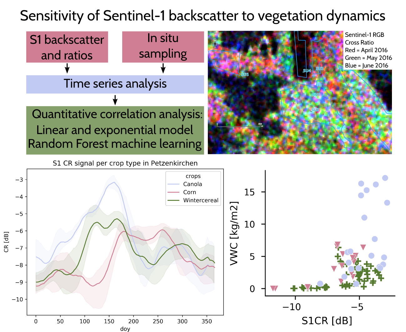
Sensitivity of Sentinel-1 Backscatter to Vegetation Dynamics: An Austrian Case Study

 , , , , ,
  and
and 
Abstract

1. Introduction
2. Data
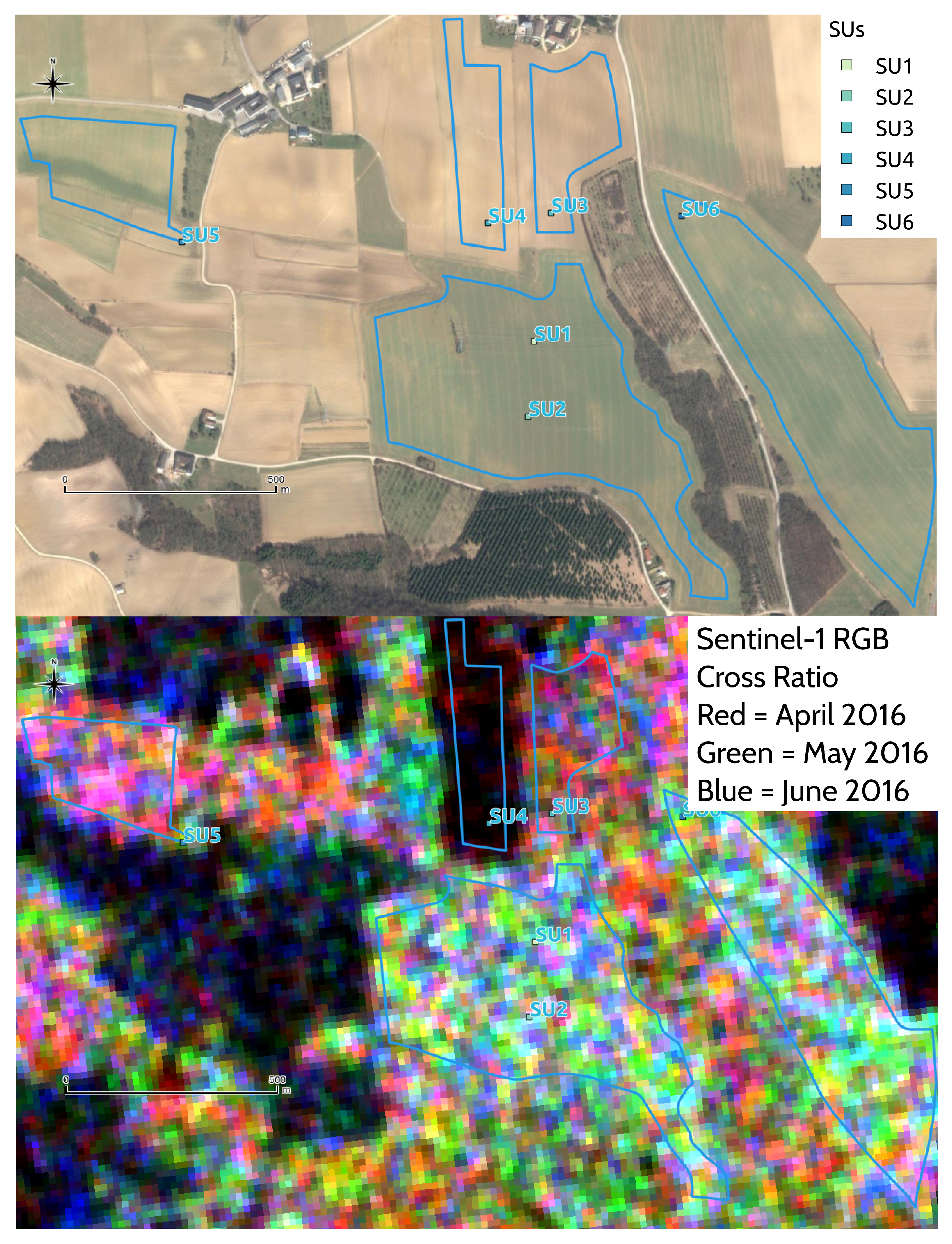
2.1. Site Description
2.2. In Situ Data
2.2.1. Biomass and Vegetation Water Content
2.2.2. Leaf Area Index
2.2.3. Vegetation Height and Status
2.2.4. Soil Moisture and Precipitation
2.3. Sentinel-1
3. Methods
3.1. Microwave Indices from Sentinel-1
3.2. Linear and Exponential Model
3.3. Random Forest Modeling
4. Results and Discussion
4.1. Time Series Analysis
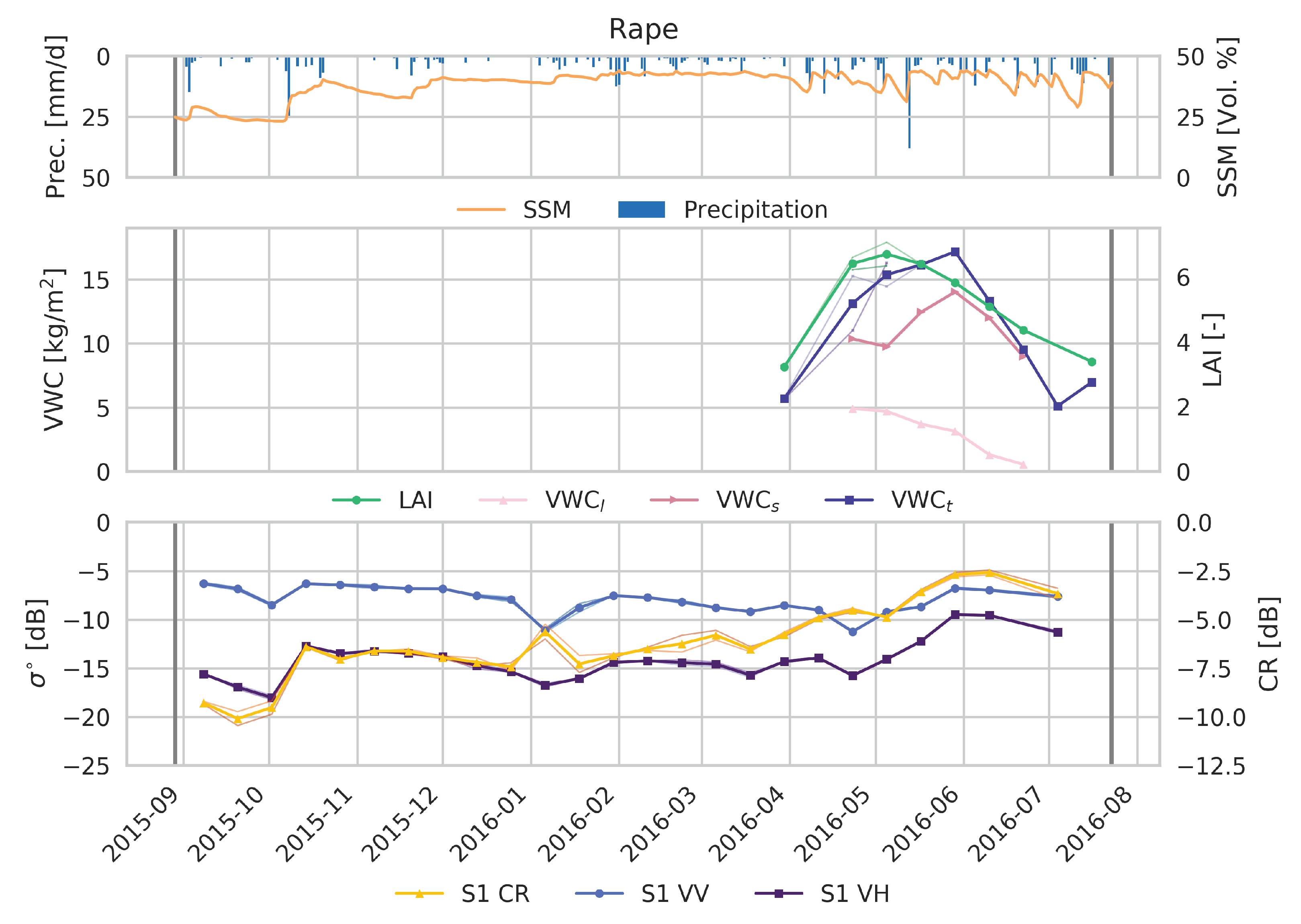
4.1.1. Oilseed-Rape
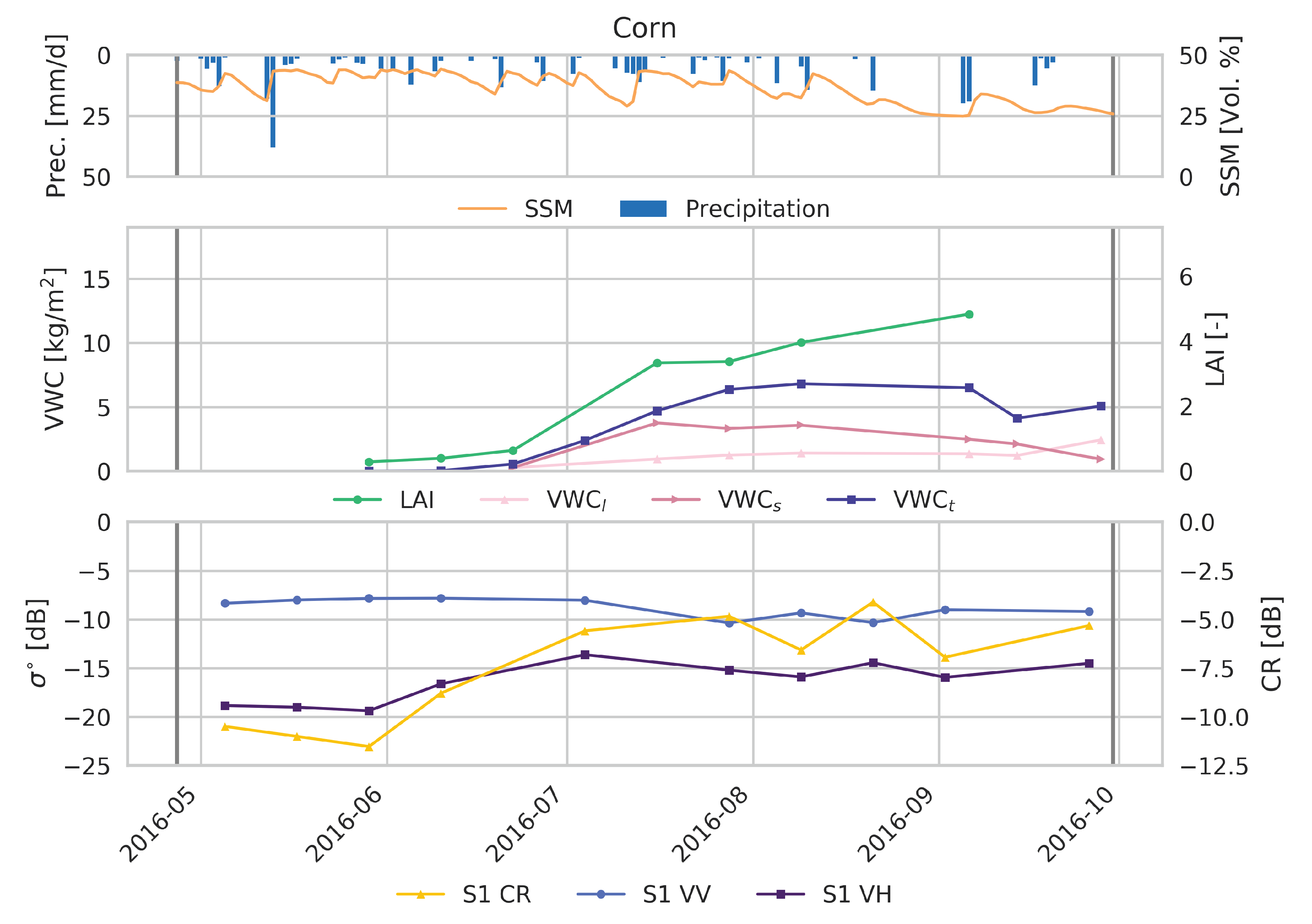
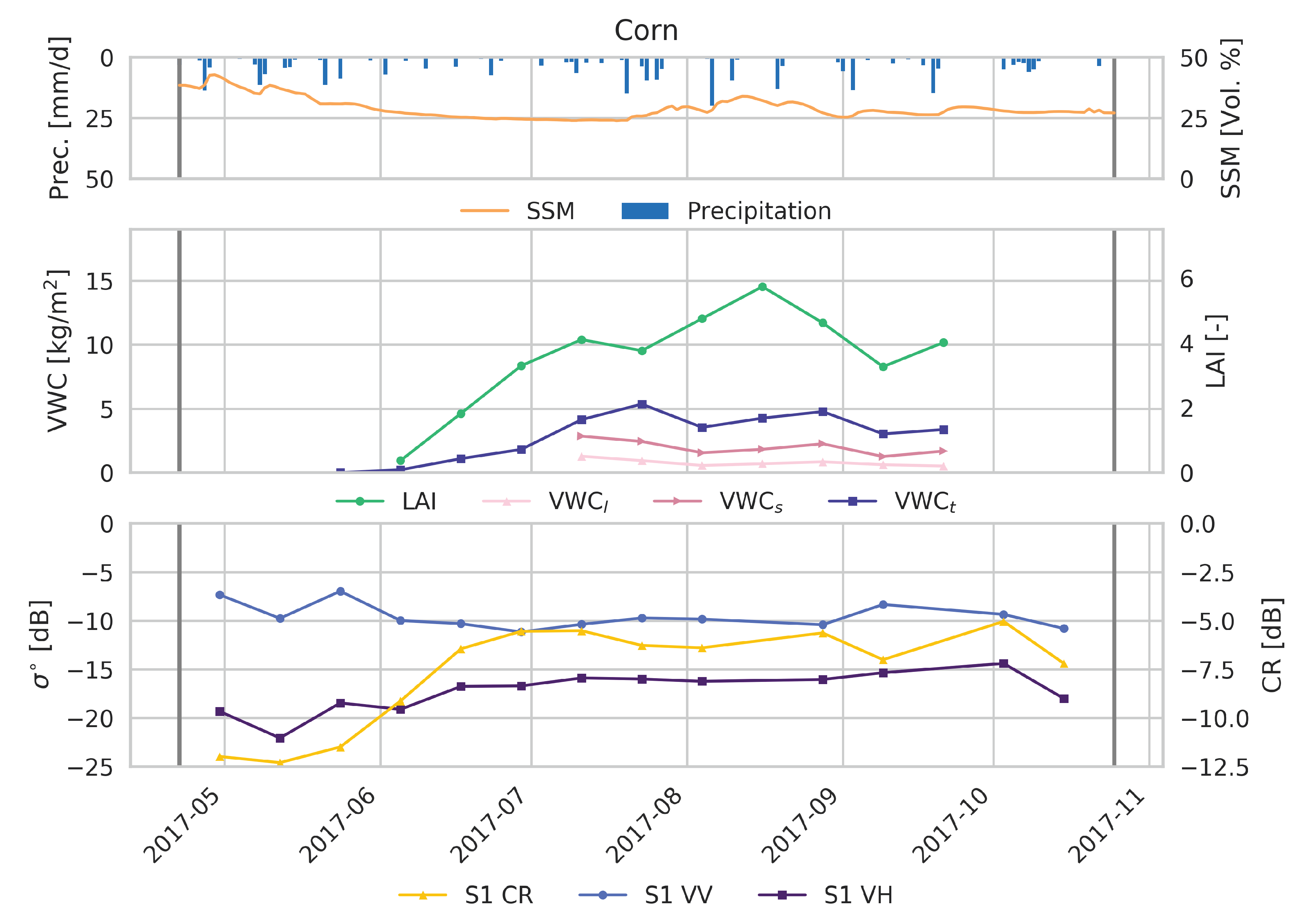
4.1.2. Corn
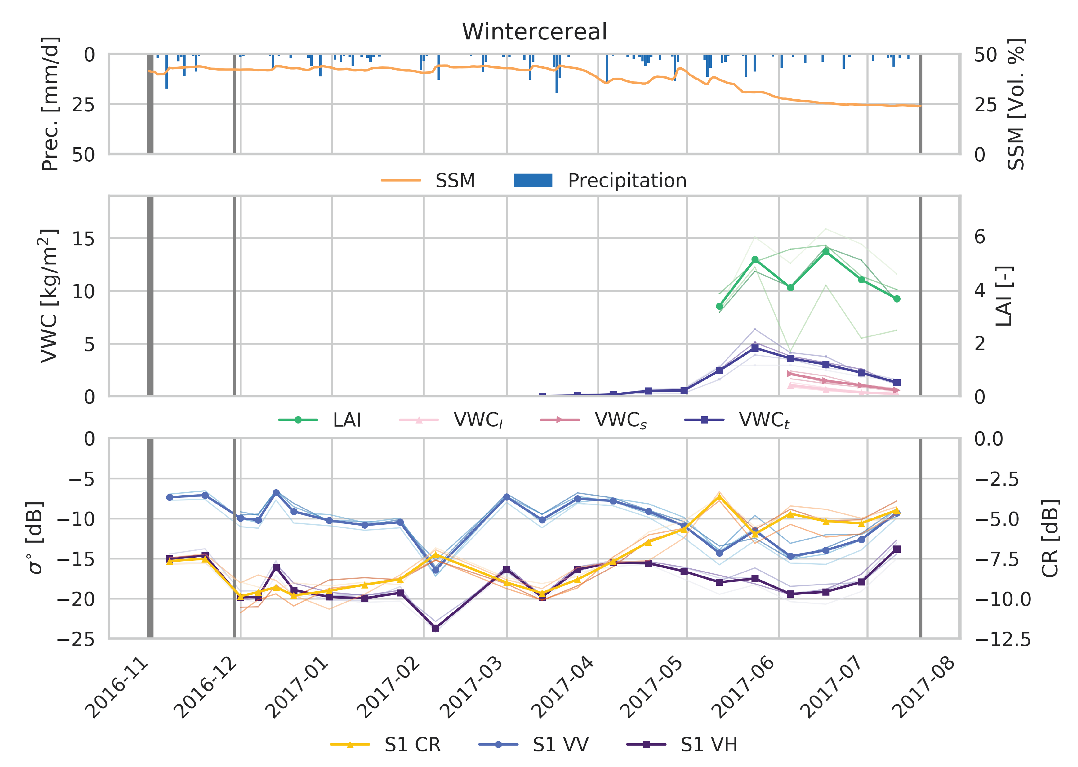
4.1.3. Winter Cereals
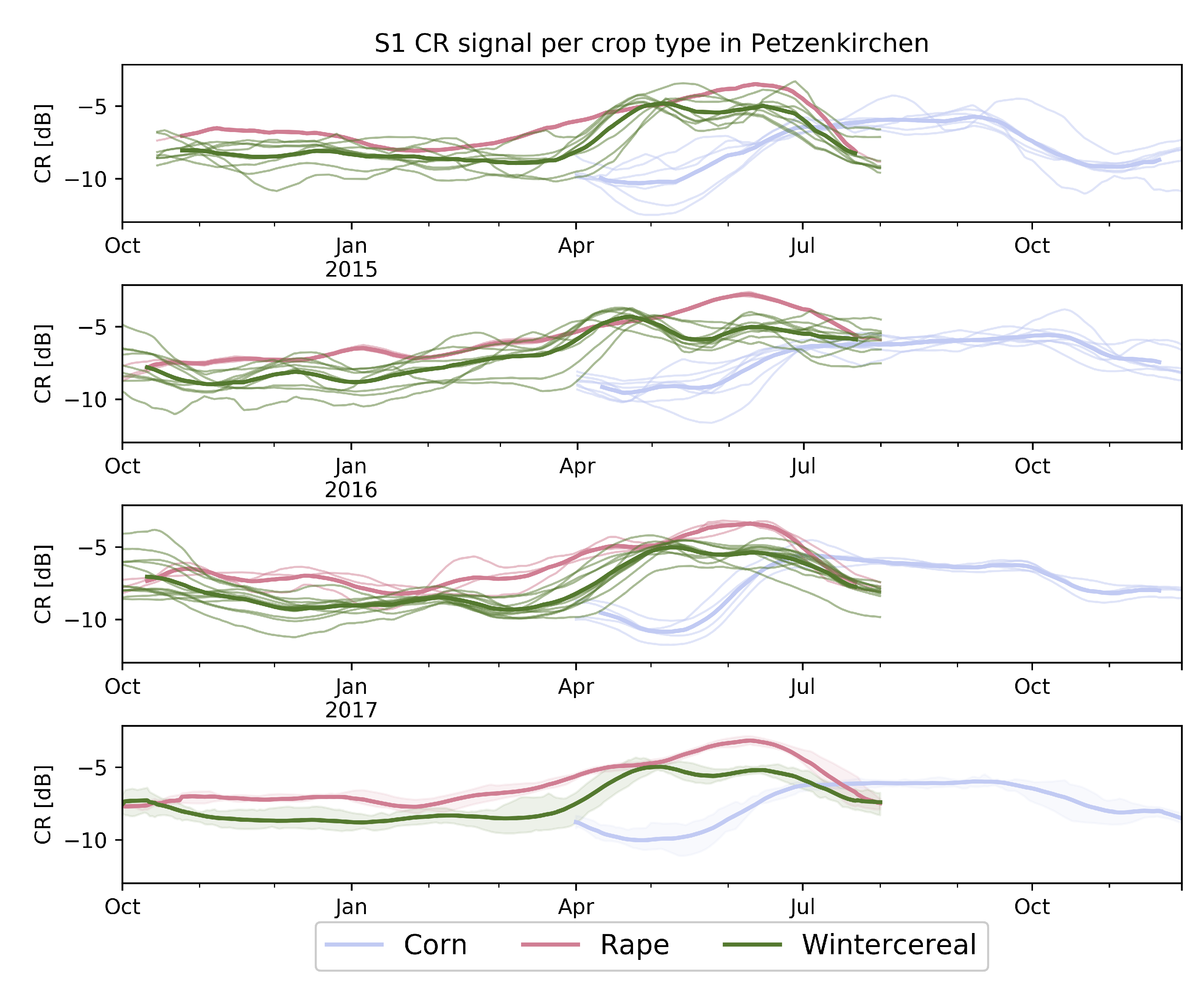
4.2. Temporal Evolution of CR
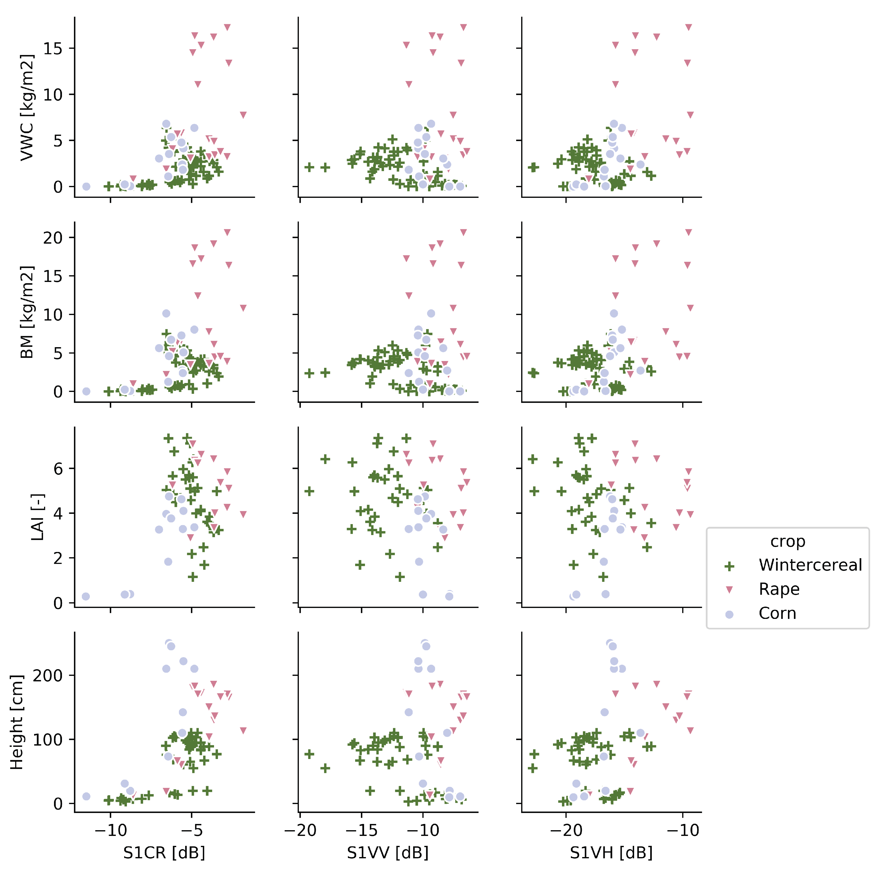
4.3. Quantitative Comparison
4.3.1. Linear and Exponential Model Results
4.3.2. Random Forest Model Results
5. Conclusions
Author Contributions
Funding
Acknowledgments
Conflicts of Interest
References
- Schmidhuber, J.; Tubiello, F.N. Global food security under climate change. Proc. Natl. Acad. Sci. USA 2007, 104, 19703–19708. [Google Scholar] [CrossRef] [PubMed]
- Godfray, H.C.J.; Beddington, J.R.; Crute, I.R.; Haddad, L.; Lawrence, D.; Muir, J.F.; Pretty, J.; Robinson, S.; Thomas, S.M.; Toulmin, C. Food security: The challenge of feeding 9 billion people. Science 2010, 327, 812–818. [Google Scholar] [CrossRef] [PubMed]
- Steele-Dunne, S.C.; McNairn, H.; Monsivais-Huertero, A.; Judge, J.; Liu, P.W.; Papathanassiou, K. Radar remote sensing of agricultural canopies: A review. IEEE J. Sel. Top. Appl. Earth Observ. Remote Sens. 2017, 10, 2249–2273. [Google Scholar] [CrossRef]
- Wagner, W.; Lemoine, G.; Rott, H. A method for estimating soil moisture from ERS scatterometer and soil data. Remote Sens. Environ. 1999, 70, 191–207. [Google Scholar] [CrossRef]
- Kerr, Y.; Waldteufel, P.; Richaume, P.; Wigneron, J.P.; Ferrazzoli, P.; Mahmoodi, A.; Al Bitar, A.; Cabot, F.; Gruhier, C.; Juglea, S.; et al. The SMOS Soil Moisture Retrieval Algorithm. IEEE Trans. Geosci. Remote Sens. 2012, 50, 1384–1403. [Google Scholar] [CrossRef]
- Parinussa, R.M.; Holmes, T.R.H.; Wanders, N.; Dorigo, W.A.; de Jeu, R.A.M. A Preliminary Study toward Consistent Soil Moisture from AMSR2. J. Hydrometeorol. 2014, 16, 932–947. [Google Scholar] [CrossRef]
- Van der Schalie, R.; Parinussa, R.M.; Renzullo, L.J.; van Dijk, A.I.J.M.; Su, C.H.; de Jeu, R.A.M. SMOS soil moisture retrievals using the land parameter retrieval model: Evaluation over the Murrumbidgee Catchment, southeast Australia. Remote Sens. Environ. 2015, 163, 70–79. [Google Scholar] [CrossRef]
- Liu, Y.Y.; de Jeu, R.A.M.; McCabe, M.F.; Evans, J.P.; van Dijk, A.I.J.M. Global long-term passive microwave satellite-based retrievals of vegetation optical depth. Geophys. Res. Lett. 2011, 38. [Google Scholar] [CrossRef]
- Jones, M.O.; Jones, L.A.; Kimball, J.S.; McDonald, K.C. Satellite passive microwave remote sensing for monitoring global land surface phenology. Remote Sens. Environ. 2011, 115, 1102–1114. [Google Scholar] [CrossRef]
- McColl, K.A.; Entekhabi, D.; Piles, M. Uncertainty analysis of soil moisture and vegetation indices using Aquarius scatterometer observations. IEEE Trans. Geosci. Remote Sens. 2014, 52, 4259–4272. [Google Scholar] [CrossRef]
- Vreugdenhil, M.; Dorigo, W.A.; Wagner, W.; Jeu, R.A.M.d.; Hahn, S.; Marle, M.J.E.v. Analyzing the Vegetation Parameterization in the TU-Wien ASCAT Soil Moisture Retrieval. IEEE Trans. Geosci. Remote Sens. 2016, 54, 3513–3531. [Google Scholar] [CrossRef]
- Ferrazzoli, P.; Paloscia, S.; Pampaloni, P.; Schiavon, G.; Solimini, D.; Coppo, P. Sensitivity of microwave measurements to vegetation biomass and soil moisture content: A case study. IEEE Trans. Geosci. Remote Sens. 1992, 30, 750–756. [Google Scholar] [CrossRef]
- Paloscia, S.; Macelloni, G.; Pampaloni, P. The relations between backscattering coefficient and biomass of narrow and wide leaf crops. In Proceedings of the 1998 IEEE International Geoscience and Remote Sensing Symposium Proceedings, Seattle, WA, USA, 6–10 July 1998; Volume 1, pp. 100–102. [Google Scholar]
- Macelloni, G.; Paloscia, S.; Pampaloni, P.; Marliani, F.; Gai, M. The relationship between the backscattering coefficient and the biomass of narrow and broad leaf crops. IEEE Trans. Geosci. Remote Sens. 2001, 39, 873–884. [Google Scholar] [CrossRef]
- Kim, Y.; Jackson, T.; Bindlish, R.; Lee, H.; Hong, S. Radar vegetation index for estimating the vegetation water content of rice and soybean. IEEE Geoscie. Remote Sensi. Lett. 2012, 9, 564–568. [Google Scholar]
- Paloscia, S.; Macelloni, G.; Pampaloni, P.; Sigismondi, S. The potential of C- and L-band SAR in estimating vegetation biomass: the ERS-1 and JERS-1 experiments. IEEE Trans. Geosci. Remote Sens. 1999, 37, 2107–2110. [Google Scholar] [CrossRef]
- Wiseman, G.; McNairn, H.; Homayouni, S.; Shang, J. RADARSAT-2 polarimetric SAR response to crop biomass for agricultural production monitoring. IEEE J. Sel. Top. Appl. Earth Observ. Remote Sens. 2014, 7, 4461–4471. [Google Scholar] [CrossRef]
- Mattia, F.; Le Toan, T.; Picard, G.; Posa, F.I.; D’Alessio, A.; Notarnicola, C.; Gatti, A.M.; Rinaldi, M.; Satalino, G.; Pasquariello, G. Multitemporal C-band radar measurements on wheat fields. IEEE Trans. Geosci. Remote Sens. 2003, 41, 1551–1560. [Google Scholar] [CrossRef]
- Satalino, G.; Balenzano, A.; Mattia, F.; Davidson, M.W. C-band SAR data for mapping crops dominated by surface or volume scattering. IEEE Geosci. Remote Sensi. Lett. 2014, 11, 384–388. [Google Scholar] [CrossRef]
- Veloso, A.; Mermoz, S.; Bouvet, A.; Le Toan, T.; Planells, M.; Dejoux, J.F.; Ceschia, E. Understanding the temporal behavior of crops using Sentinel-1 and Sentinel-2-like data for agricultural applications. Remote Sens. Environ. 2017, 199, 415–426. [Google Scholar] [CrossRef]
- Blöschl, G.; Blaschke, A.P.; Broer, M.; Bucher, C.; Carr, G.; Chen, X.; Eder, A.; Exner-Kittridge, M.; Farnleitner, A.; Flores-Orozco, A.; et al. The Hydrological Open Air Laboratory (HOAL) in Petzenkirchen: A hypothesis-driven observatory. Hydrol. Earth Syst. Sci. 2016, 20. [Google Scholar] [CrossRef]
- McNairn, H.; Hochheim, K.; Rabe, N. Applying polarimetric radar imagery for mapping the productivity of wheat crops. Can. J. Remote Sens. 2004, 30, 517–524. [Google Scholar] [CrossRef]
- Jiao, X.; McNairn, H.; Shang, J.; Pattey, E.; Liu, J.; Champagne, C. The sensitivity of RADARSAT-2 polarimetric SAR data to corn and soybean leaf area index. Can. J. Remote Sens. 2011, 37, 69–81. [Google Scholar] [CrossRef]
- Satalino, G.; Mattia, F.; Le Toan, T.; Rinaldi, M. Wheat crop mapping by using ASAR AP data. IEEE Trans. Geosci. Remote Sens. 2009, 47, 527–530. [Google Scholar] [CrossRef]
- Chala, A.; Weinert, J.; Wolf, G.A. An Integrated Approach to the Evaluation of the Efficacy of Fungicides Against Fusarium culmorum, the Cause of Head Blight of Wheat. J. Phytopathol. 2003, 151, 673–678. [Google Scholar] [CrossRef]
- Ferrazzoli, P.; Paloscia, S.; Pampaloni, P.; Schiavon, G.; Sigismondi, S.; Solimini, D. The potential of multifrequency polarimetric SAR in assessing agricultural and arboreous biomass. IEEE Trans. Geosci. Remote Sens. 1997, 35, 5–17. [Google Scholar] [CrossRef]
- Paloscia, S.; Pettinato, S.; Santi, E.; Notarnicola, C.; Pasolli, L.; Reppucci, A. Soil moisture mapping using Sentinel-1 images: Algorithm and preliminary validation. Remote Sens. Environ. 2013, 134, 234–248. [Google Scholar] [CrossRef]


| SU | Area | Crop | NS | Seeding | Harvest | St./V3 | Fl./V12 | He./R1 | Ri./R6 |
|---|---|---|---|---|---|---|---|---|---|
| 1 | 5 ha | Rape | 3 | ’15/08/29 (241) | ’16/07/23 (205) | ∼104 | ∼130 | ||
| Cereal | 11 | ’16/11/29 (334) | ’17/07/19 (200) | ∼135 | ∼150 | ∼170 | |||
| 2 | 6.1 ha | Rape | 11 | ’15/08/29 (241) | ’16/07/23 (205) | ∼104 | ∼130 | ||
| Cereal | 11 | ’16/11/29 (334) | ’17/07/19 (200) | ∼135 | ∼150 | ∼170 | |||
| 3 | 2.6 ha | Cereal | 9 | ’15/10/05 (278) | ’16/07/23 (205) | ∼100 | ∼145 | ∼165 | |
| Corn | 11 | ’17/04/22 (112) | ’17/10/25 (298) | ∼135 | ∼180 | ∼205 | ∼252 | ||
| 4 | 2.3 ha | Corn | 10 | ’16/04/27 (118) | ’16/09/30 (274) | ∼150 | ∼188 | ∼203 | ∼253 |
| Cereal | 11 | ’16/10/31 (305) | ’17/07/19 (200) | ∼135 | ∼150 | ∼170 | |||
| 5 | 3.2 ha | Cereal | 9 | ’15/10/02 (275) | ’16/07/01 (183) | ∼100 | ∼130 | ∼150 | |
| Rape | 11 | ’16/08/25 (238) | ’17/07/19 (200) | ∼100 | ∼135 | ||||
| 6 | 9.4 ha | Rape | 0 | ’15/08/28 (240) | ’16/07/20 (202) | ∼104 | ∼130 | ||
| Cereal | 11 | ’16/11/01 (306) | ’17/07/19 (200) | ∼135 | ∼150 | ∼170 |
| Crop | Model | Var | VWC | VWC | VWC | BM | LAI | H | SM |
|---|---|---|---|---|---|---|---|---|---|
| Oilseed-rape | linear | CR | 0.16 | 0.27 | 0.14 | 0.19 | 0.03 | 0.39 | 0.07 |
| VH | 0.03 | 0.29 | 0.06 | 0.05 | 0.03 | 0.15 | 0.16 | ||
| VV | 0.02 | 0.19 | 0.00 | 0.01 | 0.15 | 0.00 | 0.15 | ||
| exponential | CR | 0.34 | 0.31 | 0.36 | 0.34 | 0.08 | 0.51 | 0.06 | |
| VH | 0.10 | 0.23 | 0.12 | 0.12 | 0.01 | 0.23 | 0.16 | ||
| VV | 0.01 | 0.11 | 0.00 | 0.00 | 0.13 | 0.01 | 0.16 | ||
| Corn | linear | CR | 0.48 | 0.16 | 0.02 | 0.42 | 0.62 | 0.55 | 0.07 |
| VH | 0.44 | 0.49 | 0.16 | 0.43 | 0.61 | 0.48 | 0.00 | ||
| VV | 0.15 | 0.01 | 0.23 | 0.10 | 0.19 | 0.20 | 0.24 | ||
| exponential | CR | 0.87 | 0.18 | 0.11 | 0.85 | 0.78 | 0.83 | 0.09 | |
| VH | 0.62 | 0.35 | 0.27 | 0.63 | 0.73 | 0.61 | 0.00 | ||
| VV | 0.42 | 0.00 | 0.28 | 0.39 | 0.27 | 0.40 | 0.27 | ||
| Winter cereal | linear | CR | 0.22 | 0.34 | 0.22 | 0.26 | 0.30 | 0.50 | 0.16 |
| VH | 0.08 | 0.14 | 0.25 | 0.04 | 0.13 | 0.00 | 0.01 | ||
| VV | 0.25 | 0.04 | 0.12 | 0.22 | 0.02 | 0.21 | 0.04 | ||
| exponential | CR | 0.63 | 0.27 | 0.19 | 0.64 | 0.22 | 0.68 | 0.15 | |
| VH | 0.02 | 0.37 | 0.35 | 0.01 | 0.10 | 0.00 | 0.01 | ||
| VV | 0.35 | 0.19 | 0.38 | 0.32 | 0.01 | 0.28 | 0.04 |
| Crop | OOB Score | f1 | f2 | f3 | f4 | f5 |
|---|---|---|---|---|---|---|
| Oilseed-rape | 0.31 | S1CR | ASSM | SSM | S1VH | S1VV |
| 0.26 | 0.26 | 0.20 | 0.15 | 0.13 | ||
| Corn | 0.74 | S1CR | S1VH | ASSM | S1VV | SSM |
| 0.30 | 0.25 | 0.18 | 0.15 | 0.12 | ||
| Winter cereal | 0.81 | S1CR | ASSM | S1VV | SSM | S1VH |
| 0.31 | 0.20 | 0.18 | 0.16 | 0.16 | ||
| All | 0.80 | S1CR | S1VV | S1VH | ASSM | SSM |
| 0.35 | 0.17 | 0.16 | 0.12 | 0.11 |
© 2018 by the authors. Licensee MDPI, Basel, Switzerland. This article is an open access article distributed under the terms and conditions of the Creative Commons Attribution (CC BY) license (http://creativecommons.org/licenses/by/4.0/).
Share and Cite
Vreugdenhil, M.; Wagner, W.; Bauer-Marschallinger, B.; Pfeil, I.; Teubner, I.; Rüdiger, C.; Strauss, P. Sensitivity of Sentinel-1 Backscatter to Vegetation Dynamics: An Austrian Case Study. Remote Sens. 2018, 10, 1396. https://doi.org/10.3390/rs10091396
Vreugdenhil M, Wagner W, Bauer-Marschallinger B, Pfeil I, Teubner I, Rüdiger C, Strauss P. Sensitivity of Sentinel-1 Backscatter to Vegetation Dynamics: An Austrian Case Study. Remote Sensing. 2018; 10(9):1396. https://doi.org/10.3390/rs10091396
Chicago/Turabian StyleVreugdenhil, Mariette, Wolfgang Wagner, Bernhard Bauer-Marschallinger, Isabella Pfeil, Irene Teubner, Christoph Rüdiger, and Peter Strauss. 2018. "Sensitivity of Sentinel-1 Backscatter to Vegetation Dynamics: An Austrian Case Study" Remote Sensing 10, no. 9: 1396. https://doi.org/10.3390/rs10091396
APA StyleVreugdenhil, M., Wagner, W., Bauer-Marschallinger, B., Pfeil, I., Teubner, I., Rüdiger, C., & Strauss, P. (2018). Sensitivity of Sentinel-1 Backscatter to Vegetation Dynamics: An Austrian Case Study. Remote Sensing, 10(9), 1396. https://doi.org/10.3390/rs10091396