Estimating Fire Background Temperature at a Geostationary Scale—An Evaluation of Contextual Methods for AHI-8

Abstract

An integral part of any remotely sensed fire detection and attribution method is an estimation of the target pixel’s background temperature. This temperature cannot be measured directly independent of fire radiation, so indirect methods must be used to create an estimate of this background value. The most commonly used method of background temperature estimation is through derivation from the surrounding obscuration-free pixels available in the same image, in a contextual estimation process. This method of contextual estimation performs well in cloud-free conditions and in areas with homogeneous landscape characteristics, but increasingly complex sets of rules are required when contextual coverage is not optimal. The effects of alterations to the search radius and sample size on the accuracy of contextually derived brightness temperature are heretofore unexplored. This study makes use of imagery from the AHI-8 geostationary satellite to examine contextual estimators for deriving background temperature, at a range of contextual window sizes and percentages of valid contextual information. Results show that while contextual estimation provides accurate temperatures for pixels with no contextual obscuration, significant deterioration of results occurs when even a small portion of the target pixel’s surroundings are obscured. To maintain the temperature estimation accuracy, the use of no less than 65% of a target pixel’s total contextual coverage is recommended. The study also examines the use of expanding window sizes and their effect on temperature estimation. Results show that the accuracy of temperature estimation decreases significantly when expanding the examined window, with a 50% increase in temperature variability when using a larger window size than $5\times 5$ pixels, whilst generally providing limited gains in the total number of temperature estimates (between 0.4 and 4.4% of all pixels examined). The work also presents a number of case study regions taken from the AHI-8 disk in more depth, and examines the causes of excess temperature variation over a range of topographic and land cover conditions.

1. Introduction

Satellite remote sensing has become a vital tool in the arsenal of land managers, not only for the initial detection of active fire, but as part of inputs for modelling and planning purposes. Timely and accurate fire information from remote sensing enables preparation and planning for mitigation activities, along with providing vital information about fire behaviour and characteristics [1]. Increasing importance is being placed upon active fire products to calculate metrics such as fire radiative power and burn severity [2], in order to obtain an understanding of how the environment burns, and also to provide input for environmental modelling and quantifying outputs such as carbon emissions from fire.

Active fire detection from remote sensing relies on elevated levels of radiation in the infrared wavelengths caused by the blackbody radiation emitted from fire [2]. The typical energy emitted by fire at medium-wave infrared (3–4 $\mathsf{\mu }$$\mathrm{m}$) wavelengths can be several orders of magnitude higher than regular radiation levels, which are primarily made up of thermal emission from the surface and solar reflection [3,4]. This disparity in energy levels allow fires that are much smaller than the pixel area to be detected, as the extra energy from a fire will overwhelm the background level of radiation [1]. This propensity of fire to overwhelm the background signal presents a problem for fire detection purposes as well. The ability to determine whether a pixel is fire-affected is dependent upon knowing what the pixel should look like in the absence of fire [5]. Accurate knowledge of the differential between fire signal and background allows fire to be detected, and enables the calculation of common fire-related metrics such as fire radiative power (FRP) [6].

Without the ability to directly measure the background temperature of a pixel in the event of fire, fire algorithms have largely utilised the land area surrounding a target pixel to facilitate estimation of the background temperature, a method known as contextual estimation [6,7,8,9,10,11,12]. For pixel brightness temperatures in the medium-wave infrared, spatial autocorrelation is primarily driven by latitude, with adjacent pixels receiving similar amounts of solar radiation, along with climatic conditions, which homogenise land cover over localised regions. This was highlighted in [6], who stated that the assumption of neighbouring pixels having the same surface background characteristics was implicit in the fire algorithm developed in that work. 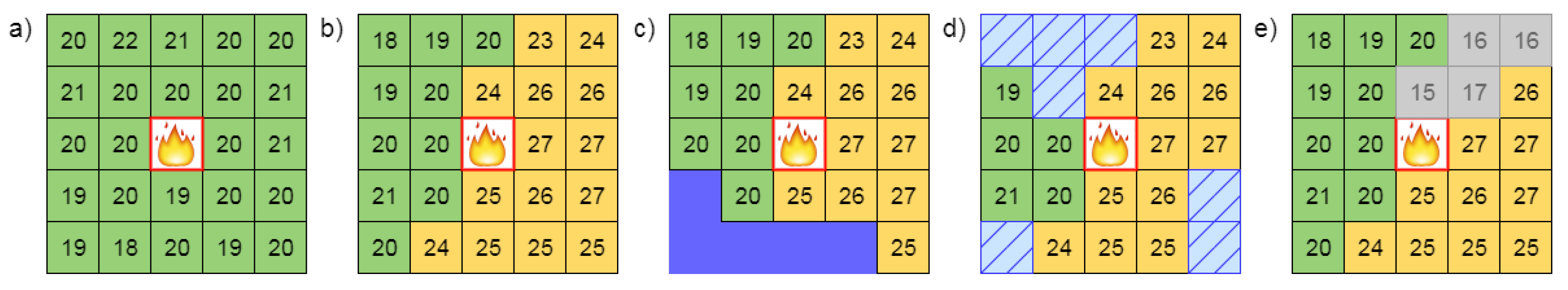This work [6] also stated that “…the extent to which this is true depends of surface spatial homogeneity and the sensor spatial resolution”. There has been no thorough examination of how surface homogeneity affects the accuracy of fire detection algorithms, despite this assumption being prevalent in active fire algorithms and products. Contextual measurements are also influenced by obscuration due to cloud or smoke, which may lead to decreased infrared radiation in pixels adjacent to a target pixel [13]. Additionally, adjacency to water bodies may eliminate some pixels from being used in contextual calculations, with islands and coastal regions particularly susceptible to errors caused by reduced land surface availability. Examples of how these scenarios may influence the calculation of background temperature may be seen in Figure 1.

Land surface temperature is a well covered topic in remote sensing [14,15,16,17,18,19], but most techniques focus upon use of thermal infrared (8–12 $\mathsf{\mu }$$\mathrm{m}$), which lacks a solar reflection component. This has led to an integration of land surface temperature techniques encompassing a combination of medium-wave and thermal infrared bands for fire detection purposes [6,9,20,21,22], due to the differential response between these two wavelengths to emitted energy from fire. Such methods rely on accurate knowledge of the sensor response to temperature in both infrared bands and their relation to one another, and often rely on arbitrary statistical thresholds to relate the two bands for detection purposes, and studies such as [23] have highlighted issues with the use of bispectral methods of fire detection. Algorithms exclusively using medium-wave infrared for background temperature detection have generally used this approach for calculation of metrics such as FRP, which is less reliant on highly accurate temperature information to achieve satisfactory results [24,25,26].

The successful launch of the AHI-8 sensor in 2015 has expanded the availability of geostationary satellite image data for the Asia-Pacific, both in the spatial and temporal resolution domains [27]. The increased spatial resolution of the sensor, which achieves 2 km × 2 km resolution in the medium-wave and thermal infrared bands, and the increased temporal coverage of the sensor, which records an as-yet unparalleled 10 $\min$ refresh rate for geostationary full disk images, provide opportunities to image and analyse the sensor’s coverage area in far greater detail than previously [28]. The fire detection and examination capabilities of the sensor have already been demonstrated in multiple studies [12,29,30,31]. These studies use a mix of contextual and multi-temporal techniques to detect and monitor fire activity, but as yet there has been no definitive fire algorithm for all conditions adopted for use with this sensor.

Fire detection algorithms perform a number of tests to not only isolate elevated sources of radiation, but to also eliminate false positive detections. Tests are usually made to mask cloud, which can trigger some detections through elevated reflectivity in the medium-wave infrared, for masking excess solar reflectivity in the form of sun glint, and to flag areas of water, which will bias infrared measurements downwards. Once these sources of error are eliminated from evaluation, decisions are then made about the suitability of pixels surrounding a potential fire for fire background temperature calculation. For instance, the MODIS MxD14 product [20] uses values initially from a 3 × 3 (3 km) pixel window surrounding the target pixel (without the leading and trailing pixels in the cross-swath direction due to pixel smearing) to determine this temperature. The algorithm then tests how many suitable contextual pixels are available for evaluation, with a successful set of target pixels isolated for temperature calculation when the number of valid contextual pixels reaches at least 25% of the total, with a minimum of eight contextual pixels used for calculation. If the algorithm cannot find sufficient pixels at the first window (in this case, only six pixels are available and eight are required), the window expands to 5 × 5 pixels, and the tests are repeated. If the test fails again, the cycle repeats expanding the window to the maximum size of 21 × 21, at which point the tests conclude with no result.

This technique of the expanding window is not exclusively used for MODIS. The VIIRS VNP14 product [32] has a background temperature calculation based upon a starting window of 11 × 11 (∼4 km in length), a success rate based on 25% of valid contextual pixels available for calculation and a 10 pixel minimum, and a maximum window range of 31 × 31 (∼10 km in length). The Fire Identification, Mapping and Monitoring Algorithm (FIMMA) for use on AVHRR sensors [33] started with a 5 × 5 window, ended at the 41 × 41 pixel level, and used 35% of total contextual pixels available with a minimum number of eight pixels used. Work involving fire detection using Landsat-8 [34] involved evaluation of a fixed 61 × 61 pixel window for background temperature calculation, with no limits placed upon the number of pixels used. Geostationary satellite algorithms apply these contextual tests as well–the MSG-SEVIRI sensor fire algorithm [6] starts at a 5 × 5 window (15 km due to the sensor spatial resolution), with a maximum window size of 15 × 15 (45 km) evaluated before calculation failure. The pixels inside each window are tested against cloud, sun glint and anomalous differences between medium-wave and thermal infrared, and only if at least 65% valid context pixels are available will an estimation take place. This work on SEVIRI has also been extended for use on the GOES sensors [17], with similar parameters used for contextual pixel utilisation.

These expanding window methods for evaluating temperature from the pixel context are applied to sensors with different spatial and radiometric characteristics, so they should differ slightly in application based upon each sensor. Despite this, apart from a rough relationship of spatial scaling between some of the products, there is no general consensus as to the ideal dimensions for contextual window evaluation, and indeed no optimal value for the minimum percentage of valid contextual pixels to use for deriving an accurate background temperature.

The objectives of this work are to examine common methods of deriving land surface temperature from a target’s surroundings in the context of fire detection. To achieve this, the enhanced temporal and spatial capabilities of the AHI-8 sensor are exploited in a large-area study. This paper presents the effects of variation of examined window sizes and valid contextual pixel percentages on background temperature. This work also highlights the challenges faced in using contextual estimation effectively, with in-depth examinations of a number of case study areas to determine the effectiveness of contextual temperature calculation.

2. Method

2.1. Data

This study utilises images from the Advanced Himawari Imager-8 (AHI-8), a geostationary sensor located at 140.7°E longitude [35], data from which was obtained from the Japan Meteorological Agency (JMA) via the Australian Bureau of Meteorology (ABOM). This geostationary sensor provides coverage over the Asia-Pacific region over 16 bands, with an image captured every 10 $\min$. Images were obtained from the $3.9$ $\mathsf{\mu }$$\mathrm{m}$ medium-wave infrared band (AHI-8 Band 7) data, which is available in Australia from the National Computing Infrastructure (NCI). Dates were randomly selected for 36 days of the year 2016, with a distribution of three per calendar month in order to provide a representative sample of times in the results. The Julian dates selected were days 6, 10, 20, 35, 36, 41, 71, 72, 82, 97, 101, 103, 133, 144, 149, 153, 164, 173, 184, 188, 200, 222, 230, 236, 253, 257, 274, 279, 286, 290, 314, 322, 323, 343, 353 and 355 of 2016. A single image was examined at each of these days for the full disk examination, which was taken at 0500 UTC. This time was selected for full disk processing to maximise the amount of the land surface in daylight, along with examination of much of the disk at, or near, peak daily temperatures. This timing also coincides with the afternoon overpass of the VIIRS sensor for much of the land areas of the disk. This study utilises a cloud mask algorithm used in a study of AHI fire detection by [30], which was adapted from use on the GOES–11 and GOES–12 geostationary sensors from [24]. This mask is calculated using AHI Bands 3, 7 and 13, along with solar zenith information at each image time, from products supplied by ABOM.

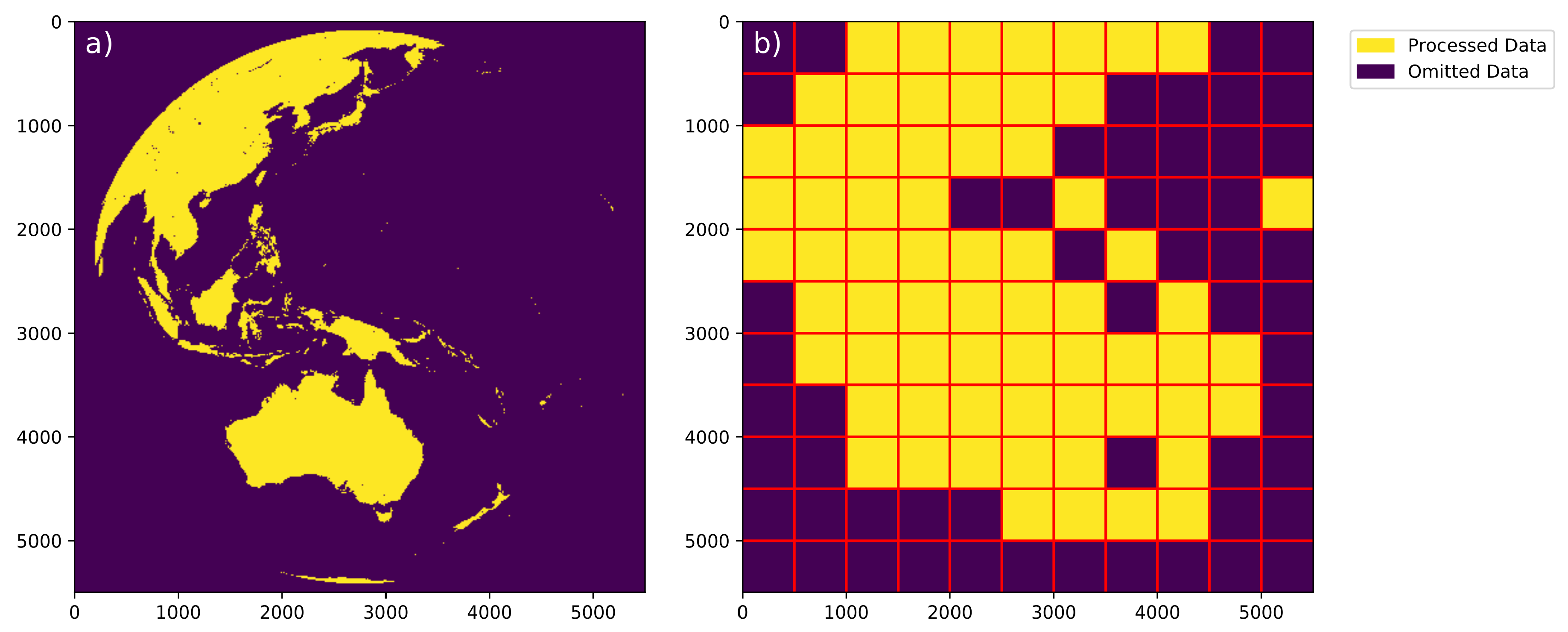
To enable efficient processing of full disk images, the size of those captured by AHI, each full disk image was divided into component arrays of 500 × 500 pixels in size. The number of land pixels in each of these component arrays was then counted, and arrays containing less than 100 land pixels were discarded from analysis. Along with these omitted areas, arrays comprising solely land constituting the continent of Antarctica were also discarded. Once these tiles were identified, selections from each image with a 12 pixel buffer (for expanding window analysis purposes) were made of each tile and processing was performed. The areas with sufficient land for analysis are shown in Figure 2.

As the focus of this study is determination of brightness temperature of land pixels, a land/sea mask supplied as part of the AHI ancillary data was applied to imagery to mask non-land pixels. Pixels close to the edge of the full disk are stretched over a large area of land surface, and also suffer from refraction due to the longer transmission period through the atmosphere. Pixels that have a sensor zenith angle greater than 80° were masked from further analysis using the AHI sensor ancillary product provided by ABOM.

2.2. AHI Disk Characterisation

Cloud is a major source of occlusion when measuring brightness temperature values. In order to obtain an understanding of the role cloud cover plays in an AHI full disk image, and by extension the distribution of clear sky pixels for analysis, the AHI image was broken into sub-images of 500 rows, for the first 5000 rows of the 5500 × 5500 image. The number of land pixels available in each of these sub-images was tallied, and the cloud coverage from the cloud mask was recorded for each full disk image. This breakdown of the AHI full disk into sub-images can be seen in the horizontal banding depicted in Figure 2b.

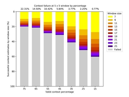
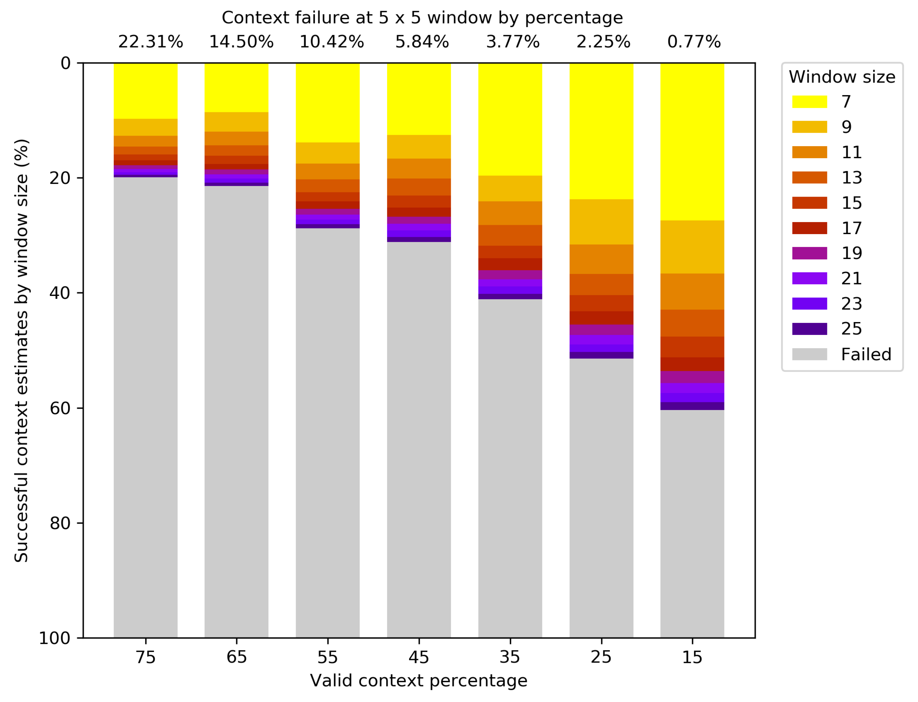
The land area covered by AHI can be quite discontinuous, especially in the equatorial regions where many islands are present. These islands and coastal areas will have permanent gaps in their contextual coverage area due to the land forms surrounding them. In order to gain an understanding of the magnitude of these standing anomalies, an analysis of the land mask was conducted. Pixels were selected by the number of contextual pixels available for estimation during a cloud-free period, and categorised into percentage classes (75%, 65%, 55%, 45%, 35%, 25%, 15%). Pixels that had less than the required percentage of pixels available on the land mask were flagged, and counts of these unusable pixels were tabled.

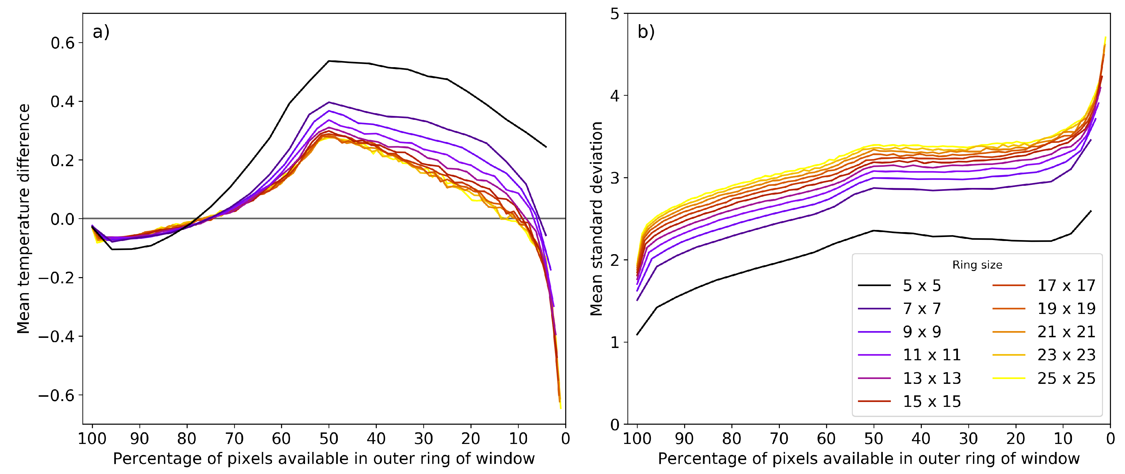
To investigate the effectiveness of contextual estimation at a full disk level, the mean of all available contextual pixels was taken for each window size for each cloud-free pixel in the 36 images selected for study. The difference between each of these contextual estimates and the benchmark central pixel was calculated, and mean and standard deviations of these differences were aggregated for analysis. These values were further broken down by the exact percentage of contextual pixels available at each window level, in order to understand how the percentage of valid pixels affects the ultimate calculation of contextual temperature.

The size of the land area covered by individual pixels in a geostationary image increases as the sensor zenith angle increases. To determine whether this expansion of pixel area has an effect on contextual temperature calculations, all pixels from the dataset with contextual estimates were then divided into classes based upon their sensor zenith angle (eight classes spanning 10° from 0 to 80°), and statistics were aggregated for each of these classes.

2.3. Expanding the Window

As noted in the introduction, there have been many approaches taken to determine a suitable window size for contextual calculation, and no general consensus has been reached for ideal parameters, apart from a rough 10 km × 10 km maximum window size for the LEO sensor algorithms. For a geostationary sensor like AHI, we are limited as to the spatial bounds of the minimum window size we can select, as the sensor resolution prevents us from resolving at better than two kilometres in the infrared bands. A minimum sampling window of $5\times 5$ has been set around each pixel, which corresponds to 10 km × 10 km at sensor nadir. A number of window sizes were examined, with values selected in two pixel increments up to a maximum window size of 25 × 25 pixels. Each of these windows had a count of valid pixels, and the mean and standard deviation of differences between the contextual mean and the central pixel value recorded for each pixel for each image.

A common feature of contextual algorithms is the use of a threshold of valid pixels as a portion of the total examination window as a limiting factor for estimation validity. If the target pixel has at least the number of valid context pixels set by this threshold, the target’s contextual pixel values are used to calculate a temperature estimate, otherwise the target is ignored. There is no consensus upon which to base a definitive decision about valid context percentage choice—the most commonly used success criterion is 25% or an arbitrary number of pixels, as used by both MODIS and VIIRS in their respective fire products. This study has chosen to examine the use of seven percentage thresholds of contextual pixel availability, ranging from 75% to 15% in 10% increments. A pixel is deemed to have sufficient contextual data to make a calculation when the number of valid contextual pixels is equal to or greater than the selected percentage over the window being examined. For example, at the 5 × 5 window size, nine or more valid pixels need to be available for a temperature to be calculated at the 35% threshold. At some thresholds, land pixels with proximity to oceans and lakes may have insufficient land available to calculate a temperature.

Another commonly utilised feature of contextual algorithms is the expanding window. When insufficient data is available at an inner window size, the window of examination grows outwards until it obtains sufficient data to make a temperature determination. For a true evaluation of the effects of the expanding window on contextual estimation, it is important to know not only how often this window expansion occurs, but the effect the expanding window has upon calculated contextual estimations. For the expanding window section of this study, the portion of data with full contextual coverage at the $5\times 5$ window was analysed separately from pixels with at least one contextual pixel obscured. From the remaining pixels for each of the valid context percentages, pixels with sufficient context available at the $5\times 5$ were identified, and statistics calculated over these pixels. For the remaining pixels with no solution at the $5\times 5$ window at each valid context percentage, the window of examination was expanded to $7\times 7$. At this point, the counts of valid context pixels were totalled for the current window and all previous windows. If the new number of contextual pixels was sufficient for the valid context percentage to be met, a contextual estimate was calculated over all contextual pixels available, and these statistics were recorded for reporting at the specified window size. After this, the examination window was expanded, and the process was repeated. Once the window of examination reached $25\times 25$, some pixels were unable to find a solution based upon the selected percentage of valid contextual pixels. Counts of these failed pixels were also recorded.

Also, some expanding window methods will in addition use an absolute threshold for the number of valid contextual pixels required for temperature estimation. Once the number of contextual pixels available satisfies this threshold of valid pixels, a contextual estimate will be made based upon the available pixels regardless of the valid context percentage set. The work presented in this paper also examined the effects of using an absolute threshold of valid pixels of 10, similar to the VIIRS VNP14 product. For this, the $5\times 5$ window was firstly analysed, and as 10 pixels was the cutoff for validity for the 45% valid pixel class at $5\times 5$, no higher valid contextual pixel percentages were examined. If a target pixel had either the required percentage of contextual pixels available, or sufficient contextual pixels to reach the absolute cutoff, the target pixel had a context temperature estimate calculated and recorded. Where this requirement was not met, the window was expanded to the next window size. If a target pixel did not reach either the valid contextual percentage or the absolute threshold of contextual pixels by the $25\times 25$ window, the target pixel was recorded as a failure and tallied.

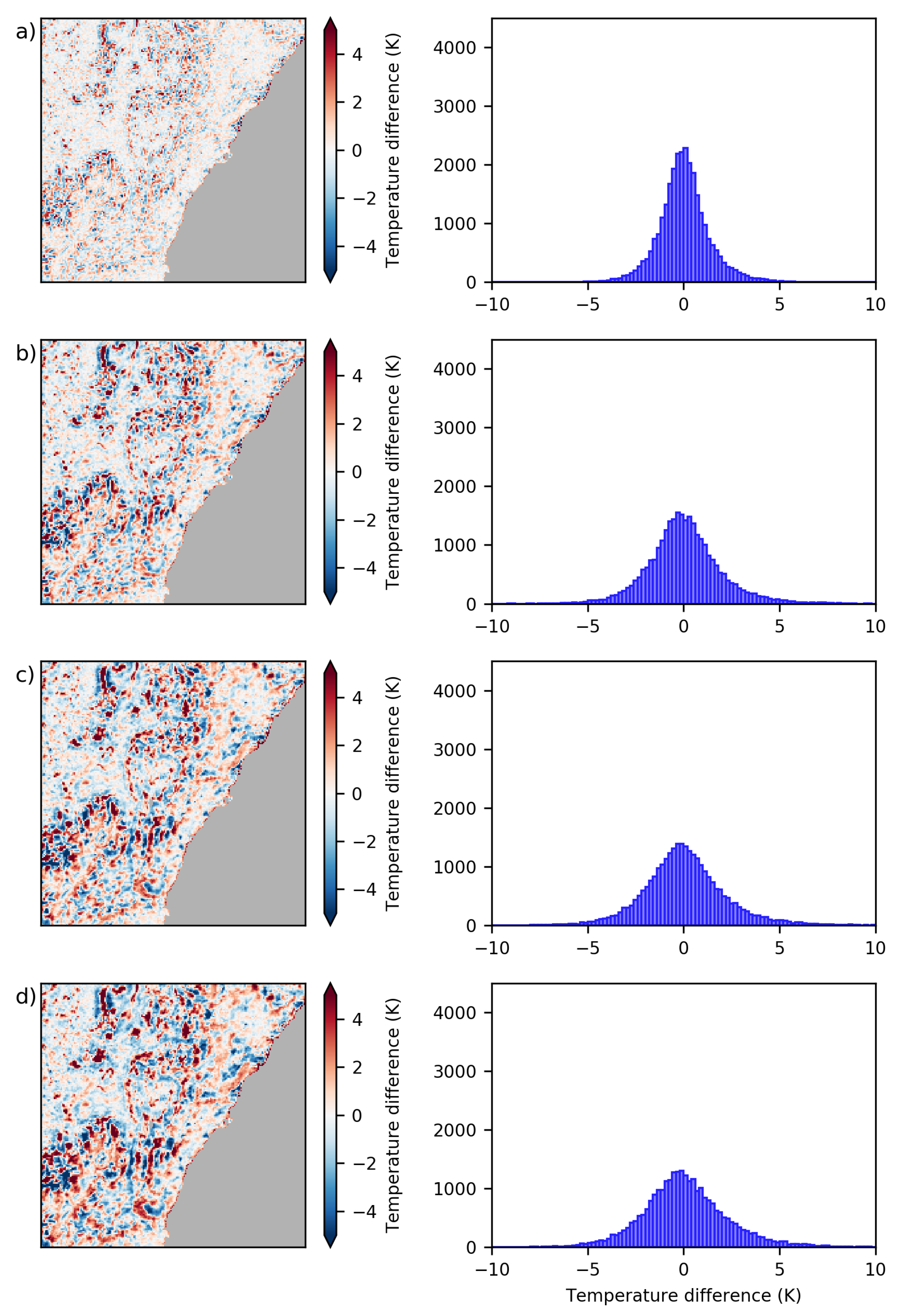
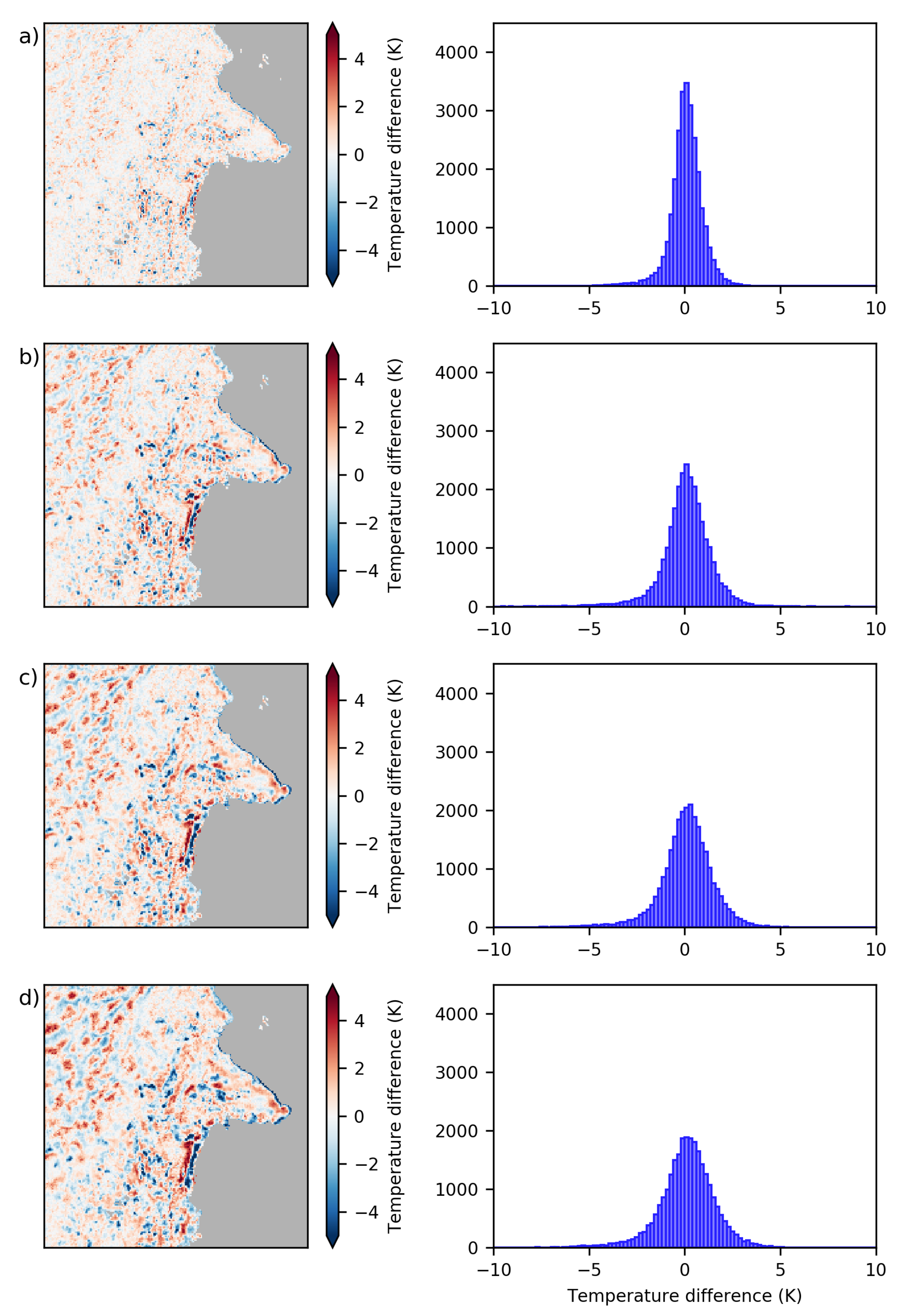
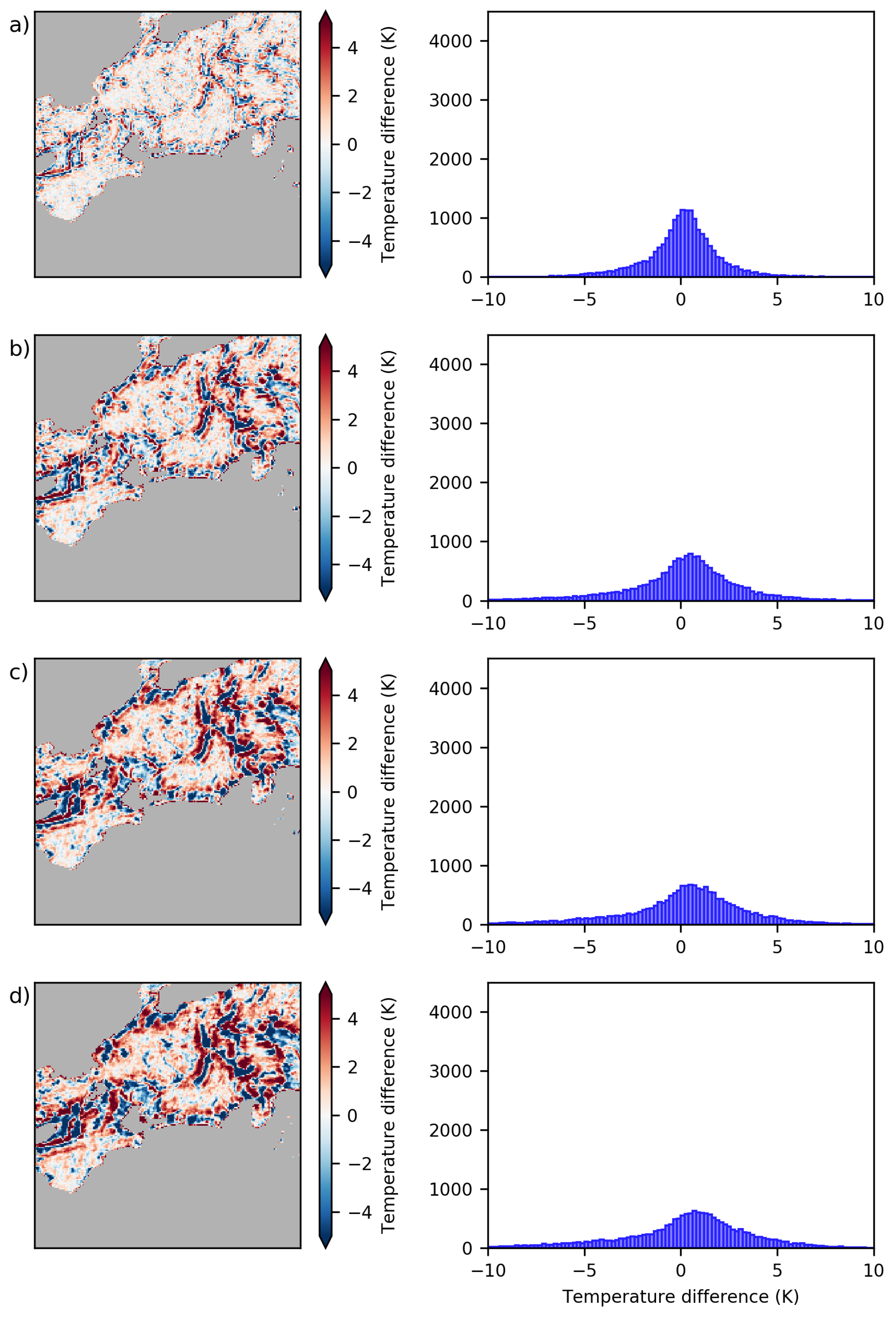
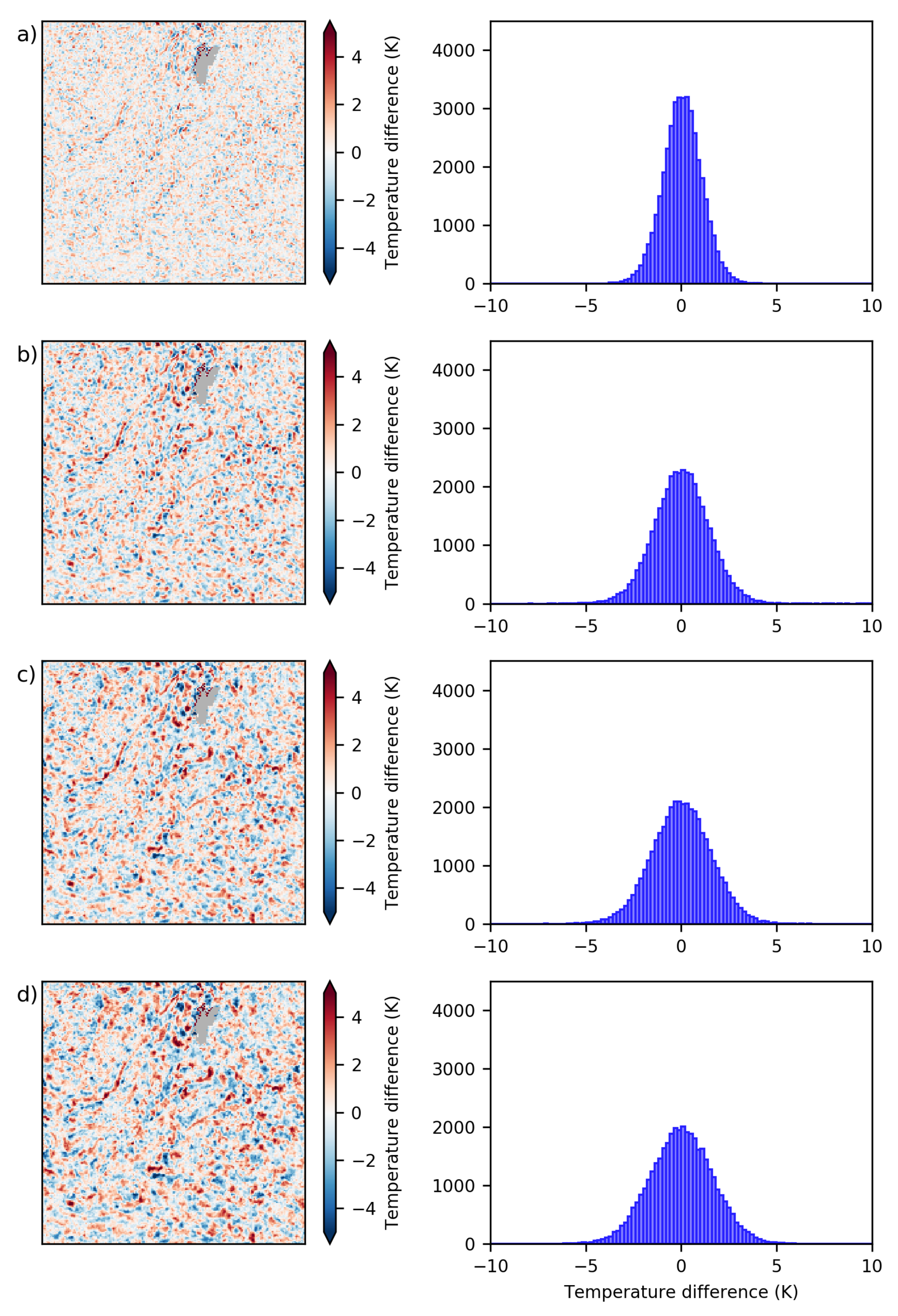
2.4. Case Study Evaluation

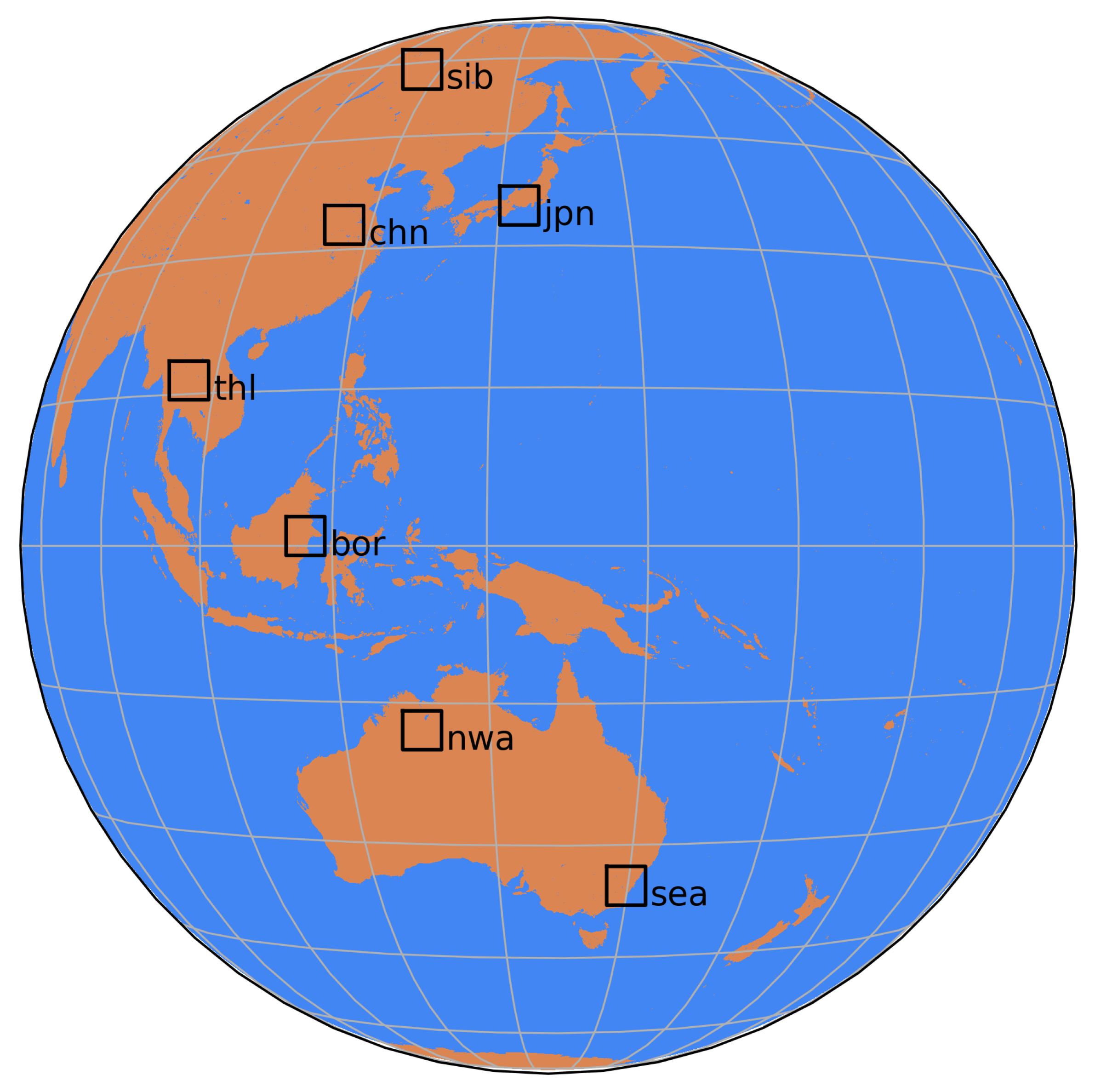
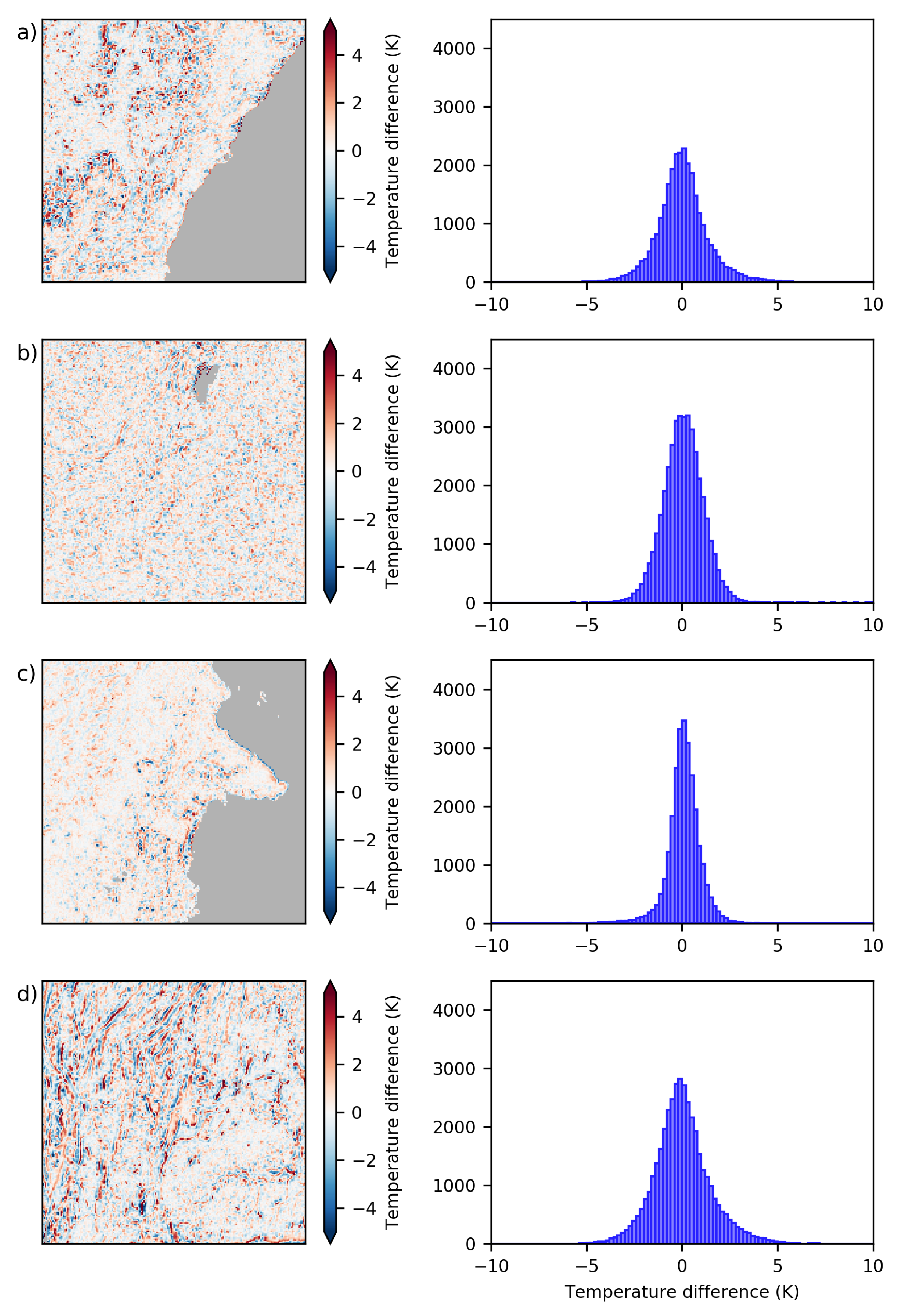
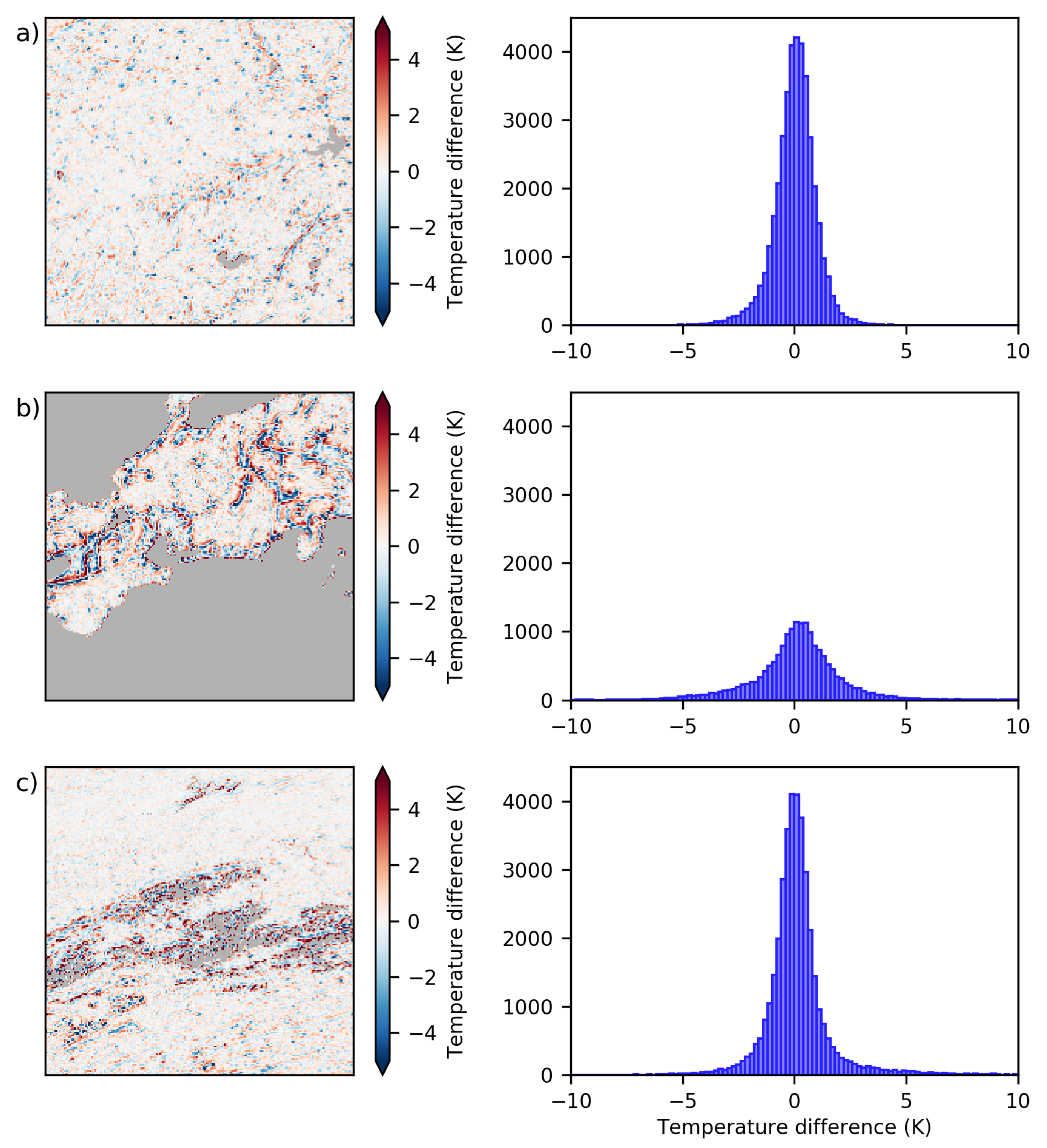
A series of case study areas have also been evaluated in a more in-depth fashion, due to their land surface variation or their fire-prone nature. These areas include part of south-eastern Australia, part of north-western Australia, a section of Kalimantan’s east coast, part of central Thailand, part of eastern China, the central part of Honshu in Japan, and part of Siberia east of Lake Baikal. Each of these areas consists of a section of the AHI image measuring 200 × 200 pixels in size, with a small buffer to provide data for pixels at the edge of the selected window. These study areas are highlighted in Figure 3.

In order to provide a more representative understanding of how each of these landscapes behaves during fire-prone periods, a selection of images for each case study area was made based upon the prevalence of fire over 2016. The monthly VIIRS fire product (VNP14IMGML) [36] was subsampled for each of the study areas, and a rolling window of 30 days was applied to the sum total of fires from each area over the course of the year. The point of time exhibiting maximum fire activity from this was then used as the central day in a 31-day window for in-depth analysis. The image time selected for each case study area was also derived from the time of fires detected during the day time period in each case study area. The selection criteria for each case study area are detailed in

Table 1. Specifications for the time frames, area of the AHI disk and UTC times for analysis of each of the case study areas.

Case Study Area	Start Date	End Date	AHI Image Area	Time (UTC)	Local Time@Centroid
sea	2016-03-30	2016-04-29	[4400, 4600, 3050, 3250]	3:50	13:49
nwa	2016-10-23	2016-11-22	[3600, 3800, 2000, 2200]	5:00	13:32
bor	2016-02-14	2016-03-15	[2600, 2800, 1400, 1600]	5:40	13:22
thl	2016-02-28	2016-03-29	[1800, 2000, 800, 1000]	6:30	13:15
chn	2016-08-27	2016-09-26	[1000, 1200, 1600, 1800]	5:10	12:56
jpn	2016-05-03	2016-06-02	[900, 1100, 2500, 2700]	3:50	12:59
sib	2016-05-10	2016-06-09	[200, 400, 2000, 2200]	5:00	12:43

.

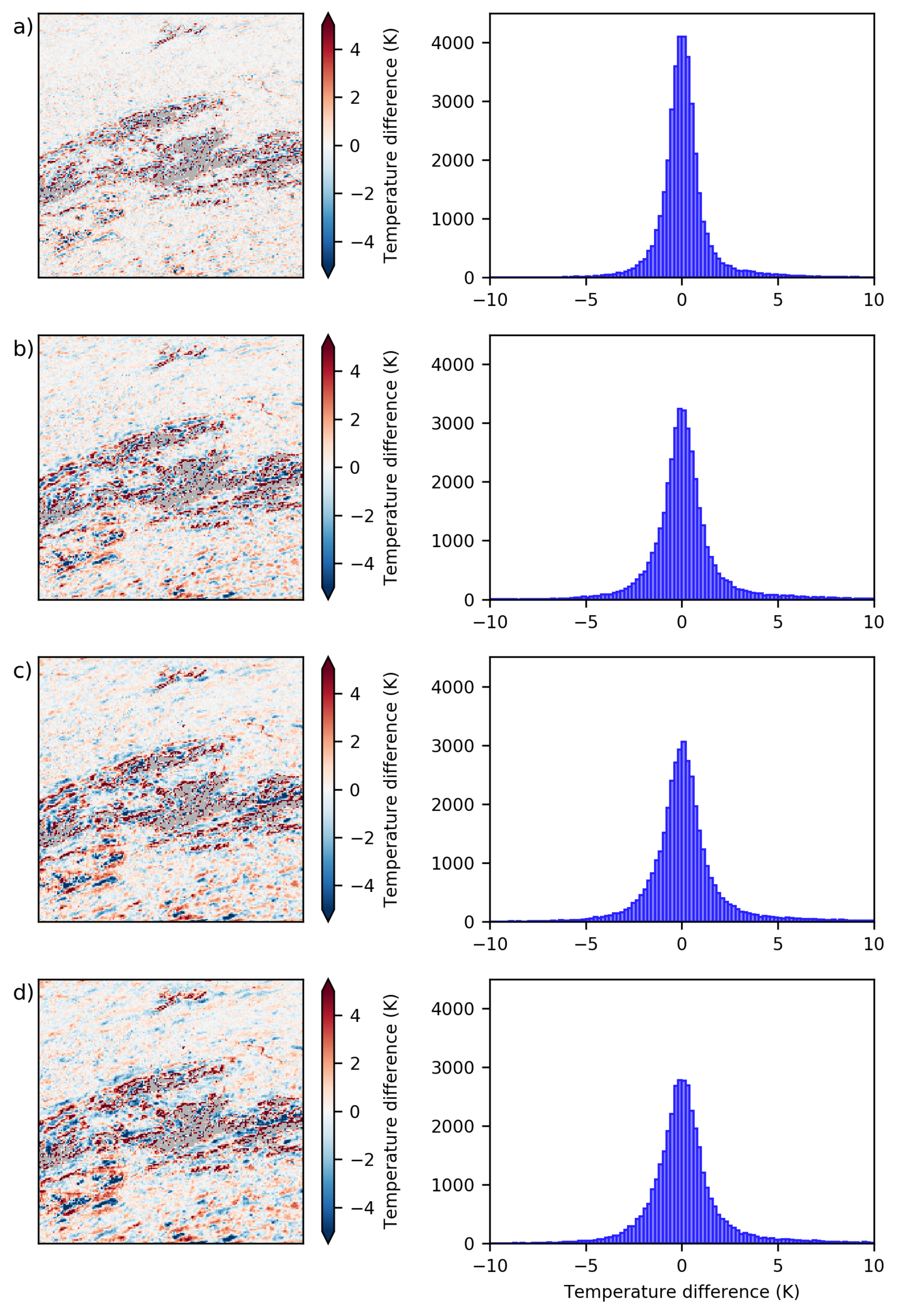
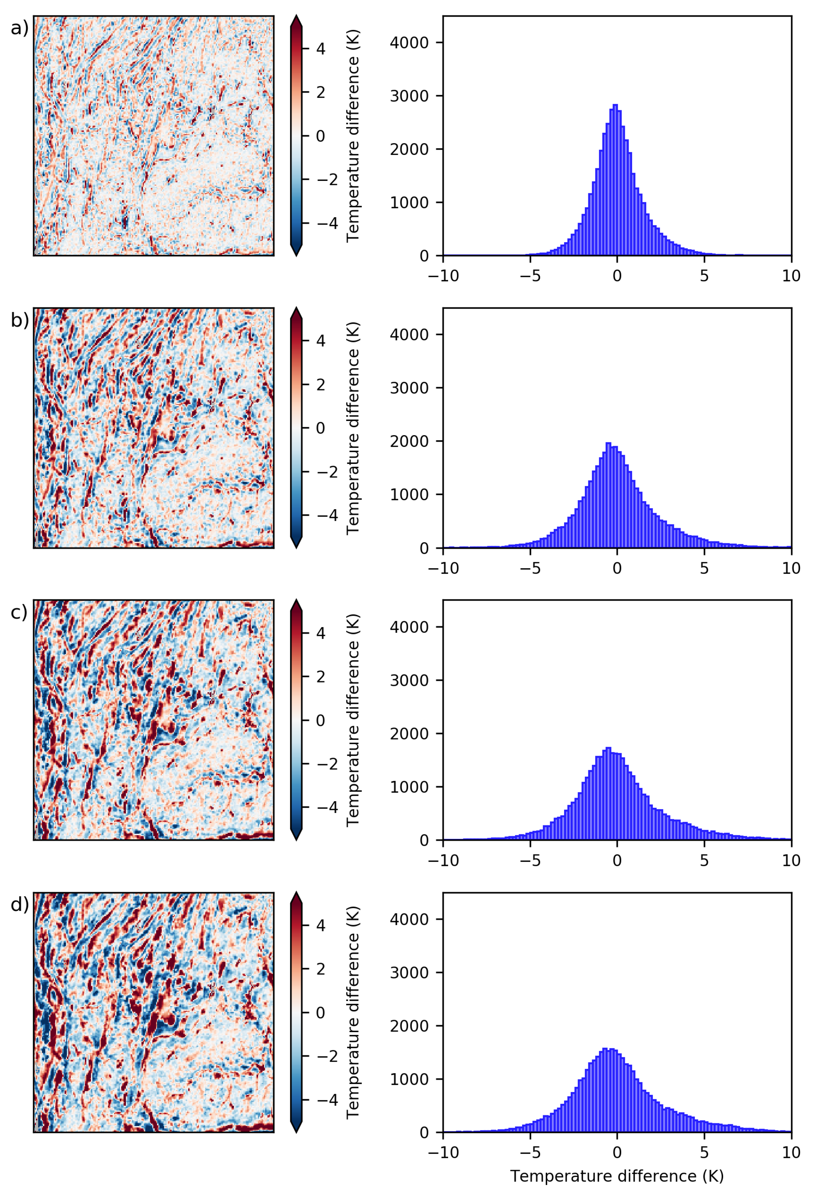
The counts of valid context pixels, and the difference of the context pixel mean from the central pixel were obtained for each window size, for each image, for each of the case study areas used for analysis. A visual examination of the causes of contextual estimate variation was also conducted based upon the spatial distribution of the mean temperature differences calculated, over window sizes from $5\times 5$ pixels to $11\times 11$ pixels, for each site.

3. Results

3.1. AHI Full Disk Characterisation

Cloud is a major impediment to any surface temperature estimation, and the area covered by the AHI disk is no exception. At the 0500 UTC time point, on average $55.6$% of assessable land surfaces on the AHI disk are covered by cloud, with cloud coverage over land surfaces ranging from 45% to 73% over the images analysed. Cloud cover is most common over the northerly quarter of the disk, with areas north of AHI image row 1500 experiencing 68–74% cloud cover over the period examined. A full breakdown of cloud cover statistics can be found in

Table 2. Average and standard deviation of cloud coverage for the AHI land areas covered in the study. The figures are an aggregate of 36 images recorded at 0500 UTC as mentioned in Section 2.1, broken into horizontal slices of the AHI disk as shown in Figure 2.

AHI Image Rows	# of Land Pixels	Mean % Cloud	SD % Cloud
0–500	526,506	74.1	15.7
500–1000	714,119	69.1	15.0
1000–1500	663,172	68.1	13.7
1500–2000	420,460	49.2	23.0
2000–2500	184,404	54.2	19.3
2500–3000	366,370	62.7	10.4
3000–3500	248,687	55.3	12.4
3500–4000	643,030	28.6	14.0
4000–4500	793,030	37.3	16.7
4500–5000	103,387	58.1	19.4

. These areas of cloud cover, as determined by the cloud mask product, were removed from the context analysis, and form the bulk of the missing data in the window examinations.

Table 3. Number and percentage of pixels that are lacking sufficient adjacent pixels to provide contextual estimation at various window sizes and percentages across the AHI disk. A total of 4,663,165 AHI land pixels were evaluated.

Window Size	Percentage of Context Pixels Required for Assessment
	>75%	>65%	>55%	>45%	>35%	>25%	>15%
$5\times 5$	103,801	74,712	46,141	18,523	10,918	4840	2389
	2.23%	1.60%	0.99%	0.40%	0.23%	0.10%	0.05%
$7\times 7$	136,747	97,771	54,351	25,771	13,842	7322	3873
	2.93%	2.10%	1.17%	0.55%	0.30%	0.16%	0.08%
$9\times 9$	165,592	110,470	61,786	31,008	17,290	9436	4544
	3.55%	2.37%	1.32%	0.66%	0.37%	0.20%	0.10%
$11\times 11$	192,298	129,744	73,595	37,000	21,033	11,510	5563
	4.12%	2.78%	1.58%	0.79%	0.45%	0.25%	0.12%
$13\times 13$	217,235	150,574	86,662	43,558	24,681	13,651	6794
	4.66%	3.23%	1.86%	0.93%	0.53%	0.29%	0.15%
$15\times 15$	240,738	165,472	97,107	49,446	28,451	15,689	7549
	5.16%	3.55%	2.08%	1.06%	0.61%	0.34%	0.16%
$17\times 17$	263,862	182,197	106,023	55,620	31,895	17,482	8466
	5.66%	3.91%	2.27%	1.19%	0.68%	0.37%	0.18%
$19\times 19$	286,131	195,443	114,230	60,973	35,605	19,496	9159
	6.14%	4.19%	2.45%	1.31%	0.76%	0.42%	0.20%
$21\times 21$	307,516	210,405	122,986	66,290	38,851	21,809	10,196
	6.59%	4.51%	2.64%	1.42%	0.83%	0.47%	0.22%
$23\times 23$	328,452	226,933	132,790	71,657	42,888	24,078	11,199
	7.04%	4.87%	2.85%	1.54%	0.92%	0.52%	0.24%
$25\times 25$	348,645	240,456	142,150	75,910	46,572	25,839	12,100
	7.48%	5.16%	3.05%	1.63%	1.00%	0.55%	0.26%

supplies a breakdown of pixels that are in permanent deficit of sufficient contextual pixels for temperature estimation at each valid context percentage at each window size. A requirement of at least 75% of contextual pixel availability is quite restrictive given the landforms present, and at least $2.2$% of all land pixels cannot obtain this number of adjacent contextual pixels in the $5\times 5$ window. The numbers in this table are adjusted for all window levels preceding—an assessment of a $7\times 7$ window for instance takes into account pixels at the $5\times 5$ window at the same time to determine whether an estimation is possible over all of the context pixels available to the target. These target pixels suffer permanent obscuration, and these locations can be flagged as problematic for contextual calculation for all periods.

Table 4. Mean and standard deviation of the contextual estimate differences from central brightness temperature (AHI Band 7) for all available pixels in the 36-day set of full disk images at 0500 UTC. A total of 76,023,810 pixels were examined over the 36 images used in the study.

Window Size	5 × 5	7 × 7	9 × 9	11 × 11	13 × 13	15 × 15
mean (K)	0.037	0.031	0.029	0.027	0.025	0.024
std (K)	1.522	2.039	2.200	2.320	2.415	2.494
count	76,023,810	75,858,159	75,871,580	75,880,469	75,888,096	75,893,762
Window Size	17 × 17	19 × 19	21 × 21	23 × 23	25 × 25
mean (K)	0.023	0.023	0.023	0.024	0.024
std (K)	2.562	2.622	2.677	2.726	2.771
count	75,895,983	75,899,037	75,899,238	75,898,553	75,898,041

shows the global mean and standard deviation for all target pixels available for assessment at each window level individually. This assessment is conducted where there is at least one contextual pixel available at the denoted window size for comparison. As can be seen, there is a global tendency to overestimate temperature from the available contextual pixels, and there is little change in central tendency once the window of examination grows beyond $11\times 11$. The variation of the temperature estimation rises with the increased distance of assessed pixels from the centre, although the distance from the central pixel becomes less of an influence on variation once the window of examination grows beyond $11\times 11$. Global statistics such as these hide some of the more interesting trends in the data, and Figure 4 shows the breakdown of mean and standard deviation by contextual pixel availability at each window.

Figure 4a shows the mean value of the temperature difference as a function of the valid context percentage available at the outer edge of each window, apart from at the 5 × 5 window, where analysis includes all pixels inside this window. When all pixels are available for analysis at a particular window edge, the distance of the examined pixels from the central pixel has no influence upon the resulting temperature estimate, and the difference between estimates calculated using pixels from each window edge stays similar down to 75% of available pixels. At this point, having fewer pixels available in the 5 × 5 window of pixels causes a growth in temperature overestimation, which reaches a maximum when half of adjacent pixels are unavailable.

Figure 4b shows the standard deviation of the temperature difference as a function of the percentage of contextual pixels available, similar to Figure 4a. For all window sizes, the standard deviation suffers a large increase once only one value is obscured in a window, with this effect most marked at the larger window sizes. Variation peaks in a similar fashion to the mean at around half of all contextual pixels available, with most window sizes seeing a levelling out of variation until only a handful of contextual pixels remain for estimation. The relative indifference to distance from the central pixel for the larger window sizes is due to the way pixels here are selected for analysis. The outer edge of the specified window is assessed, which is square in shape, and the pixels at each outer edge exhibit a far greater range of distances from the central pixel as one moves further out, which would smooth out any purely distance-based variation.

The investigation into the effect of sensor zenith angle on temperature estimation found no marked influence. Mean values in the 5 × 5 window for temperature differences ranged from $0.07$ $\mathrm{K}$ in the 0–10° view angle region, down to $0.025$ $\mathrm{K}$ near the edge of the disk between 70° and 80° zenith angle over the images analysed. The largest errors were present in the two regions closest to nadir (0–10° and 10–20°), but the land surface area in these regions is much smaller than further out from the sensor nadir. There are no trends present due to sensor zenith angle in the standard deviation of contextual estimation either, apart from a slight drop in values close to nadir and at the 70–80° zenith angle.

3.2. Expanding Window Analysis

Table 5. Mean and standard deviation of brightness temperature differences between the central pixels and the contextual surrounds at each window level per percentage level. Numbers shown in the 5 × 5 window row report statistics for pixels that would be added to the 1.00 pixels if the valid context percentage shown was used to accept contextual estimates. The percentage of total pixels with estimates available at the 5 × 5 window for each valid context percentage is also shown. The rows for each subsequent window size describe the number of temperature estimations that would be added from failures at the previous window size by expanding the examined window, and the subsequent means and variances of pixels included from these window sizes. A total of 76,023,810 pixels were examined over the 36 images used in the study.

Window		1.00	Valid Portion of Total Context Pixels
			0.99–0.75	0.99–0.65	0.99–0.55	0.99–0.45	0.99–0.35	0.99–0.25	0.99–0.15
5 × 5	mean ($\mathrm{K}$)	−0.029	−0.083	−0.036	0.006	0.063	0.086	0.100	0.111
	std ($\mathrm{K}$)	1.090	1.603	1.699	1.759	1.839	1.867	1.885	1.898
	count	40,958,274	18,106,490	24,041,100	27,144,999	30,622,724	32,199,899	33,351,687	34,480,202
	% avail	53.88%	23.82%	31.62%	35.71%	40.28%	42.36%	43.87%	45.35%
Total 5 × 5 success			77.69%	85.50%	89.58%	94.16%	96.23%	97.75%	99.23%
7 × 7	mean ($\mathrm{K}$)	–	0.474	0.772	0.925	1.059	1.029	0.995	0.940
	std ($\mathrm{K}$)	–	2.314	2.538	2.667	2.734	2.711	2.705	2.768
	count	N/A	1,651,297	948,803	1,096,828	557,910	562,891	407,382	160,575
	% avail	N/A	2.17%	1.25%	1.44%	0.73%	0.74%	0.54%	0.21%
9 × 9	mean ($\mathrm{K}$)	–	0.704	1.007	1.143	1.293	1.270	1.193	1.143
	std ($\mathrm{K}$)	–	2.592	2.778	2.874	2.932	2.908	2.914	2.999
	count	N/A	502,591	369,619	289,271	182,700	127,933	134,785	53,782
	% avail	N/A	0.66%	0.49%	0.38%	0.24%	0.17%	0.18%	0.07%
11 × 11	mean ($\mathrm{K}$)	–	0.889	1.193	1.341	1.498	1.476	1.381	1.310
	std ($\mathrm{K}$)	–	2.757	2.940	3.050	3.075	3.086	3.054	3.197
	count	N/A	320,616	262,912	221,789	155,173	118,434	87,380	36,791
	% avail	N/A	0.42%	0.35%	0.29%	0.20%	0.16%	0.11%	0.05%
13 × 13	mean ($\mathrm{K}$)	–	1.024	1.321	1.491	1.615	1.611	1.521	1.471
	std ($\mathrm{K}$)	–	2.860	3.055	3.161	3.200	3.228	3.221	3.348
	count	N/A	228,249	199,477	177,211	130,197	102,158	63,145	27,398
	% avail	N/A	0.30%	0.26%	0.23%	0.17%	0.13%	0.08%	0.04%
15 × 15	mean ($\mathrm{K}$)	–	1.137	1.445	1.597	1.739	1.726	1.600	1.551
	std ($\mathrm{K}$)	–	2.982	3.165	3.252	3.273	3.286	3.325	3.410
	count	N/A	174,901	158,520	121,066	93,067	63,103	48,553	21,233
	% avail	N/A	0.23%	0.21%	0.16%	0.12%	0.08%	0.06%	0.03%
17 × 17	mean ($\mathrm{K}$)	–	1.224	1.585	1.702	1.830	1.804	1.765	1.626
	std ($\mathrm{K}$)	–	3.032	3.283	3.333	3.371	3.436	3.437	3.449
	count	N/A	139,247	108,539	105,588	70,645	58,638	38,539	14,115
	% avail	N/A	0.18%	0.14%	0.14%	0.09%	0.08%	0.05%	0.02%
19 × 19	mean ($\mathrm{K}$)	–	1.328	1.694	1.818	1.953	1.875	1.834	1.702
	std ($\mathrm{K}$)	–	3.177	3.358	3.414	3.445	3.450	3.507	3.610
	count	N/A	113,322	93,057	79,027	54,876	46,985	31,733	12,024
	% avail	N/A	0.15%	0.12%	0.10%	0.07%	0.06%	0.04%	0.02%
21 × 21	mean ($\mathrm{K}$)	–	1.416	1.747	1.867	2.046	2.020	1.885	1.805
	std ($\mathrm{K}$)	–	3.265	3.380	3.471	3.556	3.573	3.595	3.866
	count	N/A	94,179	81,879	71,265	51,677	33,939	27,491	10,239
	% avail	N/A	0.12%	0.11%	0.09%	0.07%	0.04%	0.04%	0.01%
23 × 23	mean ($\mathrm{K}$)	–	1.422	1.817	1.951	2.043	2.040	1.948	1.911
	std ($\mathrm{K}$)	–	3.288	3.502	3.572	3.591	3.657	3.646	3.883
	count	N/A	80,631	73,046	63,430	48,480	36,557	23,016	9168
	% avail	N/A	0.11%	0.10%	0.08%	0.06%	0.05%	0.03%	0.01%
25 × 25	mean ($\mathrm{K}$)	–	1.547	1.877	2.025	2.079	2.110	1.988	2.024
	std ($\mathrm{K}$)	–	3.342	3.548	3.549	3.575	3.661	3.556	3.886
	count	N/A	70,008	64,301	51,988	40,127	27,803	20,150	8127
	% avail	N/A	0.09%	0.08%	0.07%	0.05%	0.04%	0.03%	0.01%
Total failures			13,584,005	8,664,283	5,643,074	3,057,960	1,687,196	831,675	231,882
			17.87%	11.40%	7.42%	4.02%	2.22%	1.09%	0.31%

demonstrates the breakdown of estimated pixel values when utilising an expanded window algorithm. Firstly, the rate reported in the 1.00 column represents the characteristics of pixels that have all contextual pixels available at the 5 × 5 window. These pixels, which make up $53.88$% of all cloud-free pixels analysed, are generally underestimated by contextual methods, albeit only by $0.03$ $\mathrm{K}$, and display low variance. The other columns in the 5 × 5 row report statistics on the pixels that are added at each of the contextual percentage availabilities specified. For example, if a process accepted estimates with 45% or more available contextual pixels, an extra $40.28$% of all target pixels would be available for evaluation, in addition to the $53.88$% from the full context (1.00) pixels. The additional pixels accepted at each valid context percentage have the means and standard deviations shown. For the remaining pixels without a solution, the examined contextual window is expanded through the window values shown, with statistics reported for pixels that achieve the valid context percentage at each window size. After the process is exhausted at the 25 × 25 window, the remaining pixels without a solution for each percentage are tallied in the total failures row at the bottom of the table.

The tendency of a target pixel’s contextual surrounds to slightly underestimate temperature in optimal conditions, as seen in Figure 4, is also seen here in the 5 × 5 section of Table 5. As the threshold for valid contextual pixels is lowered, the mean temperature of all estimates rises and the variation in these estimates increases. Of course, these trade-offs in temperature accuracy come with an increased level of coverage—accepting 65% contextual pixel availability allows $85.5$% of all target pixels to be estimated with a neutral mean and relatively low variance. Conversely, accepting pixels at 15% contextual availability would allow for the calculation of temperature estimates over $99.2$% of all target pixels, but with both higher mean and higher variance overall. Once the window of contextual pixels is expanded though, the accuracies coming from the contextual estimate deteriorate. In general, the pixel’s context tends to overestimate temperatures by an increasing amount, with mean temperature differences ranging between 0.47 and 2.11 $\mathrm{K}$, and the standard deviation of results increases by around 50% by just moving from a 5 × 5 window to a 7 × 7 window of examination.

A further examination of calculation rates using the expanded window sizes is shown in Figure 5. For the portion of pixels that have no solution at the 5 × 5 window for each percentage, this figure shows the proportion of target pixels that subsequently obtain sufficient valid contextual pixels for calculation at each window size. The portion of target pixels that does not achieve sufficient contextual pixel counts for evaluation after expansion to the 25 × 25 window is shown in grey. As seen in Table 5, the higher contextual limitations have larger portions of the total data set that suffer from insufficient data for estimation. Changing the acceptance percentage does not, however, affect the proportion of pixels that subsequently obtain sufficient contextual pixels for estimation at larger window sizes. This figure shows that no expanding window threshold will return values for more than $60.3$% of the remaining pixels that fail to be calculated at the 5 × 5 window size, with the 75% threshold yielding less than 20% of extra pixels at larger windows. Of the pixels that do manage to obtain solutions, on average at least $69.5$% of those occur at the 11 × 11 window size or lower, and $83.4$% occur at window sizes at, or smaller than, 15 × 15. This rate of return for the expanding window method, coupled with the variability of results coming from estimations made at the larger window sizes, calls into question the overall effectiveness of using such a method, especially considering the computationally intensive nature of using pixels from a wider area.

Often in the case of some of the LEO fire products, an absolute cutoff threshold is used in order to calculate temperatures where a certain number of pixels are available for the calculation, regardless of their distance from the central pixel. A table demonstrating the effect of using a valid pixel threshold of 10 or more pixels is shown in

Table 6. Mean and standard deviation of brightness temperature differences between the central pixels and the contextual surrounds at each window level per percentage level, or where the number of context pixels reaches 10. The 5 × 5 window statistics show the global rates for pixels which have equal or greater contextual pixels than the minimum for estimation. The rows for each window size describe the number of calculated values that would be added by expanding to each window size, and the subsequent means and variances of pixels included from these window sizes.

Window		1.00	Valid Portion of Total Context Pixels
			0.99–0.45	0.99–0.35	0.99–0.25	0.99–0.15
5 × 5	mean ($\mathrm{K}$)	−0.029	0.076	0.086	0.100	0.111
	std ($\mathrm{K}$)	1.090	1.856	1.867	1.885	1.898
	count	40,958,274	31,473,186	32,199,899	33,351,687	34,480,202
	% avail	53.88%	41.40%	42.36%	43.87%	45.35%
Total 5 × 5 success			95.27%	96.23%	97.75%	99.23%
7 × 7	mean ($\mathrm{K}$)	–	0.709	0.746	0.874	0.940
	std ($\mathrm{K}$)	–	2.550	2.568	2.642	2.768
	count	N/A	2,456,495	1,734,495	664,734	160,575
	% avail	N/A	3.23%	2.28%	0.87%	0.21%
9 × 9	mean ($\mathrm{K}$)	–	0.623	0.628	0.703	0.996
	std ($\mathrm{K}$)	–	2.639	2.640	2.673	2.928
	count	N/A	591,757	589,044	531,807	97,775
	% avail	N/A	0.78%	0.77%	0.70%	0.13%
11 × 11	mean ($\mathrm{K}$)	–	0.544	0.548	0.588	0.854
	std ($\mathrm{K}$)	–	2.723	2.723	2.745	2.963
	count	N/A	225,018	224,240	212,723	119,473
	% avail	N/A	0.30%	0.29%	0.28%	0.16%
13 × 13	mean ($\mathrm{K}$)	–	0.485	0.487	0.518	0.701
	std ($\mathrm{K}$)	–	2.789	2.792	2.816	2.971
	count	N/A	108,023	107,653	103,138	66,691
	% avail	N/A	0.14%	0.14%	0.14%	0.09%
15 × 15	mean ($\mathrm{K}$)	–	0.448	0.451	0.481	0.637
	std ($\mathrm{K}$)	–	2.828	2.831	2.852	3.018
	count	N/A	60,176	59,952	57,566	39,017
	% avail	N/A	0.08%	0.08%	0.08%	0.05%
17 × 17	mean ($\mathrm{K}$)	–	0.413	0.414	0.435	0.584
	std ($\mathrm{K}$)	–	2.844	2.845	2.869	3.019
	count	N/A	37,688	37,596	36,118	24,821
	% avail	N/A	0.05%	0.05%	0.05%	0.03%
19 × 19	mean ($\mathrm{K}$)	–	0.401	0.403	0.434	0.562
	std ($\mathrm{K}$)	–	2.864	2.867	2.897	3.057
	count	N/A	25,000	24,899	23,883	16,827
	% avail	N/A	0.03%	0.03%	0.03%	0.02%
21 × 21	mean ($\mathrm{K}$)	–	0.439	0.441	0.464	0.607
	std ($\mathrm{K}$)	–	2.996	3.000	3.031	3.226
	count	N/A	17,483	17,419	16,712	12,002
	% avail	N/A	0.02%	0.02%	0.02%	0.02%
23 × 23	mean ($\mathrm{K}$)	–	0.316	0.318	0.341	0.428
	std ($\mathrm{K}$)	–	2.913	2.919	2.943	3.092
	count	N/A	12,125	12,068	11,667	8478
	% avail	N/A	0.02%	0.02%	0.02%	0.01%
25 × 25	mean ($\mathrm{K}$)	–	0.304	0.306	0.324	0.415
	std ($\mathrm{K}$)	–	2.869	2.874	2.897	2.998
	count	N/A	8910	8867	8596	6289
	% avail	N/A	0.01%	0.01%	0.01%	0.01%
Total failures			49,675	49,404	46,905	33,386
			0.07%	0.06%	0.06%	0.04%

. This table does not show valid percentages above 45%, as pixels that are only valid at these higher percentages trigger the absolute pixel threshold at the 5 × 5 window. The 10 pixel threshold homogenises the 45%, 35% and 25% classes to an extent, with very similar means and standard deviations emerging from each window size. Setting an absolute threshold of valid pixels does increase the total number of pixels that obtain temperature estimates, but even so there is still a number of pixels for which a solution is not possible, even at the lowest percentages. In comparison to the figures presented in Table 5, the estimated means at the higher window percentages using the absolute threshold are reduced, and the variation of temperature estimates smooths out once the window expands beyond $9\times 9$. This is due to more pixels in the original analysis expanding the window further than what was required to provide a reasonably accurate temperature estimation. The major improvement from using an absolute pixel threshold is in the total percentage of pixels that are assessable, with the first two window sizes able to provide estimates in ≥98% of cases in all percentage classes.

3.3. Case Study Areas

Figure 6 and Figure 7 show the spatial distribution in the mean of the temperature differences at the 5 × 5 window for each of the case study areas, along with a histogram of the counts of these temperature differences per area. Each of the case study areas displays a unique distribution. South-east Australia (Figure 6a), Thailand (Figure 6d) and Japan (Figure 7b) show marked linear features which line up with boundaries of land use areas. South-eastern Australia area has the most variation in the west where forested areas are open to grazing and croplands, whilst Thailand and Japan have the greatest variation in line with changes in relief. The Japan case study area has the most variation at the tree line high on Honshu’s central range. The effect of coastline pixels is most evident in the Borneo area (Figure 6c), with the influence of swamp and mangrove along the coastline leading to an underestimation of temperatures in adjacent pixels. Urban areas are also a source of underestimation, most prevalent in the central China study area (Figure 7a) where cities in the north-west of the area display a heat island effect. This effect is also seen to a lesser extent in the south-east Australia and Japan study areas. The Siberian (Figure 7c) area displayed relative uniformity outside of the central latitudes, where unmelted snow from mountain ranges caused commission errors in the cloud mask used, which led to large estimation errors on these interfaces. North-western Australia (Figure 6b) is characterised by high local variability, and high contrast between vegetated and bare earth areas coupled with the lack of surface moisture increases this local variability (shown in greater detail in Figure A4). All distributions of temperature differences are relatively uniform in nature, with the Japan, Siberia and Thai areas displaying longer tails than other areas.

Table 7. Mean and standard deviation of the mean brightness temperature differences of each case study area for each 31-day period. Pixel values were averaged over the 31-day period for each site, and global means and standard deviations of these averages are reported.

Window Edge	5 × 5		7 × 7		9 × 9		11 × 11
Case Study Area	$\overline{\mathit{x}}$ Mean	$\overline{\mathit{x}}$ SD	$\overline{\mathit{x}}$ Mean	$\overline{\mathit{x}}$ SD	$\overline{\mathit{x}}$ Mean	$\overline{\mathit{x}}$ SD	$\overline{\mathit{x}}$ Mean	$\overline{\mathit{x}}$ SD
sea	0.031	1.312	0.051	1.891	0.063	2.090	0.079	2.229
nwa	0.059	1.031	0.024	1.440	0.022	1.570	0.021	1.658
bor	0.089	0.856	0.089	1.231	0.097	1.360	0.101	1.454
thl	0.022	1.481	0.021	2.202	0.023	2.469	0.024	2.673
chn	0.023	0.942	0.024	1.348	0.020	1.494	0.014	1.605
jpn	0.092	1.928	0.140	2.862	0.162	3.259	0.178	3.553
sib	0.112	1.370	0.134	1.810	0.144	1.939	0.152	2.026

depicts the global mean and standard deviations of the case study areas compared to the outer edge of pixels at various window sizes. The general trend of overestimation of pixel temperatures when looking at the global statistics is shown here, but the change in mean values is different from area to area. Stability in the mean temperatures here is a function of the amount of clear sky present during the times examined—Thailand, for instance, has a comparatively small number of pixels affected by cloud during the examined period, whereas Japan and Siberia are heavily cloud affected during their examined time periods. North-western Australia shows marked improvement in temperature recovery when looking at the more distant window edges, which is seemingly due to poor performance at the 5 × 5 window size. All areas have a notable gain in the temperature variance as the pixels examined become more distant from the central pixel.

Table 8. Mean and standard deviation of brightness temperature differences between the central pixels and the contextual surrounds at the specified percentage levels for the 5 × 5 window in each case study area. Each column reports the statistics of accepting the available pixels above the denoted percentage level. Pixels with full contextual coverage are reported in the 1.00 column.

			Valid pOrtion of Total Context Pixels
		1.00	0.99–0.75	0.99–0.65	0.99–0.55	0.99–0.45	0.99–0.35	0.99–0.25	0.99–0.15	All
sea	mean ($\mathrm{K}$)	−0.021	−0.042	−0.013	0.010	0.043	0.056	0.063	0.068	0.022
	std ($\mathrm{K}$)	1.670	1.832	1.862	1.880	1.921	1.931	1.935	1.941	1.804
	count	279,250	152,220	210,297	243,132	284,703	308,590	330,486	363,534	688,739
	% avail	40.5%	22.1%	30.5%	35.3%	41.3%	44.8%	48.0%	52.8%
nwa	mean ($\mathrm{K}$)	−0.051	−0.134	−0.035	0.034	0.127	0.171	0.198	0.218	0.061
	std ($\mathrm{K}$)	1.377	2.576	2.769	2.856	2.953	2.992	3.014	3.029	2.216
	count	548,125	258,015	339,147	382,837	438,487	470,677	499,270	538,353	1,129,978
	% avail	48.5%	22.8%	30.0%	33.9%	38.8%	41.7%	44.2%	47.6%
bor	mean ($\mathrm{K}$)	−0.106	−0.096	−0.038	0.003	0.051	0.071	0.086	0.096	0.061
	std ($\mathrm{K}$)	1.121	1.472	1.585	1.651	1.719	1.746	1.764	1.777	1.681
	count	90,734	250,567	343,181	392,122	451,781	485,259	515,552	559,085	702,114
	% avail	12.9%	35.7%	48.9%	55.8%	64.3%	69.1%	73.4%	79.6%
thl	mean ($\mathrm{K}$)	−0.033	0.000	0.047	0.079	0.109	0.118	0.122	0.125	0.016
	std ($\mathrm{K}$)	1.679	1.874	1.920	1.941	1.961	1.965	1.967	1.970	1.776
	count	683,361	224,582	281,720	310,807	346,989	367,880	386,865	415,359	1,134,791
	% avail	60.2%	19.8%	24.8%	27.4%	30.6%	32.4%	34.1%	36.6%
chn	mean ($\mathrm{K}$)	−0.032	−0.041	0.006	0.039	0.079	0.092	0.100	0.104	0.021
	std ($\mathrm{K}$)	1.159	1.310	1.345	1.370	1.407	1.418	1.424	1.428	1.272
	count	428,453	176,040	232,020	262,412	301,287	324,324	346,985	384,005	868,807
	% avail	49.3%	20.3%	26.7%	30.2%	34.7%	37.3%	39.9%	44.2%
jpn	mean ($\mathrm{K}$)	−0.019	−0.151	−0.134	−0.056	0.079	0.102	0.116	0.125	0.046
	std ($\mathrm{K}$)	2.061	2.246	2.269	2.332	2.460	2.479	2.486	2.490	2.265
	count	120,759	54,546	74,758	86,968	103,879	114,110	124,201	141,136	288,787
	% avail	41.8%	18.9%	25.9%	30.1%	36.0%	39.5%	43.0%	48.9%
sib	mean ($\mathrm{K}$)	−0.057	−0.073	−0.017	0.020	0.066	0.080	0.088	0.092	0.037
	std ($\mathrm{K}$)	1.120	1.746	1.814	1.859	1.947	1.969	1.980	1.996	1.745
	count	86,220	66,918	97,011	117,111	149,287	173,672	202,360	260,949	478,458
	% avail	18.0%	14.0%	20.3%	24.5%	31.2%	36.3%	42.3%	54.5%

reports statistics for each of the case study areas broken down by valid contextual pixel percentage. As can be seen in all areas, pixels with all contextual pixels available for calculation tend to underestimate the target temperature. An increasing tendency to overestimate temperature as the amount of contextual pixels available reduces is present at all sites. The stability of temperature estimation from a pixel with no contextual obscuration is also much better than from areas that are partially obscured. Some of the case study areas display a much larger variance once contextual pixels become partially obscured—the north-western Australia area is the median for variance during full availability, but is the worst performer once the contextual area is even slightly obscured. The trend of greater overestimation as obscuration of contextual pixels increases is caused by the target pixel temperature dropping due to cloud shadows causing lower solar reflectivity, in comparison to clearer and brighter valid pixels in the surroundings. The expected deterioration of accuracy for each of the percentage windows is seen clearly, with standard deviations increasing as more obscured estimations are accepted. The south-east Australia, Thailand and China areas display less variation than other areas as the percentage of valid contextual availability decreases. With regard to the number of target pixel estimates available at each contextual percentage, these examples display a slight inflection in their trend around 45%, with the number of estimates available increasing in greater quantities below this percentage and at lesser quantities above. Total recovery rates by percentage can be calculated by adding the percentage availability to the obscuration-free contextual (1.00) values.

Moving further away from the central pixel has the most marked effect on temperature variation, and this effect can be seen in Figure 8. This figure depicts the changes in the spatial and statistical distribution of contextual temperatures over the south-eastern Australian study area, for window sizes between 5 × 5 pixels and 11 × 11 pixels. Expanding the window of examination for pixel estimation exacerbates the edge effects seen in the eastern and south-eastern portions of this area, with much larger areas of high variation than on the boundaries seen previously. The greater window size also highlights the larger variations at the urban interfaces of Sydney and the Illawarra region, and shows a general overestimation of temperatures along the coastline. The distributions of temperatures remain normal, but are flattened considerably compared to values from the most adjacent pixels. Supplementary figures showing these effects in the other case study areas can be found in Appendix A.

4. Discussion

Whilst the numbers presented in Section 3.1 are specific to the AHI disk coverage area, the same factors that restrict calculation of background temperature should be common to any part of the globe where fire detection and attribution occurs. Cloud coverage is a major inhibiting factor in any satellite fire detection setup, and areas that display even moderate occlusion of the contextual surroundings tend to present less than ideal estimations of temperature. From the range of values of contextual availability shown in Figure 4a, there seems to be a break between results derived from pixels with at least 65% contextual availability and results from pixels with less contextual values available. The usage of estimates from target pixels with at least 65% available contextual information minimises the bias in the mean calculation of background temperature, especially at the larger window sizes, whilst also limiting the variation of the resultant estimations. The results presented in both Table 4 and Figure 4 also demonstrate the relative stability of temperatures derived from window sizes larger than $13\times 13$, or in AHI scale once pixels are at least 12 km from the pixel being estimated. If an increase in variance of calculated estimates of 60% over values derived at the $5\times 5$ is acceptable for a specific purpose, then there is seemingly no reason not to set the initial area of examination for contextual temperature as large as practicable, but if this temperature variance is more of a concern, then using pixels from outside even the $11\times 11$ window of pixels becomes problematic.

The effects at play when calculating contextual estimates as shown in Figure 4 bear further examination. The relative differences between the mean and variation seen at the higher window sizes reduces as the pixels examined increase in distance from the target, an effect noted in Section 3.1 being due to variations in the window edge radius. Examination of the effect of using pixels with similar distances to the target, in a circular ring, would most likely bear this out, though implementation of such a distance-based window of examination would become less trivial as sensor zenith angle increases. The pattern of mean difference as a function of valid pixels is worth mentioning as well, especially with regard to overestimation of the target temperature when valid contextual pixels approach 50%. This effect is likely due to shadowing of the target pixel and consequent reduction in solar reflectivity, with the target pixel most likely being immediately adjacent to the obscuration affecting the surrounding pixels. This effect is lessened in the rings of pixels situated further from the target pixel, as the source of obscuration at the outer edge of the window is less likely to be present closer in to the target pixel. This overestimation is not particularly large in magnitude, and is less likely to affect fire detection for instance, but such information may assist in the adjustment of temperature-controlled metrics calculated from these estimates.

The results also cast the use of expanding windows for contextual temperature examination in a poor light, particularly for those sensors with larger spatial resolutions. The vast majority of all pixel calculations are achieved at the $5\times 5$ window, with the recovery of data from using an expanding window ranging from 20% to 54% of all remaining target pixels. If we are to use the 65% window as an example, 85% of data is contributed from the $5\times 5$ window, extra estimates from using the expanding window are just over 4%, and the majority of those extra estimates occur at or below the $11\times 11$ window. There are also compromises involved in using the estimates, with a general positive bias and much higher variation in values at even the $7\times 7$ level. Depending on the purpose of using these estimates, using the data coming from the combined windows could be detrimental to the overall reporting accuracy. When evaluating how a background temperature method should be implemented, care needs to be taken to ensure that any need for comprehensive coverage, whether it be achieved by either using a smaller percentage of valid contextual pixels, by using larger window sizes, or both, does not inhibit the accuracy of the overall product.

With regard to the case study areas selected for analysis, the reasons for major variances in contextually determined temperature are as diverse as the case study sites selected. Phenomena affecting contextual estimation range from highly ephemeral conditions, such as fire and flooding, to seasonally changing influences such as snow and vegetation cover, to semi-permanent influences such as urban–rural interfaces and land cover change, and on to permanent conditions such as relief, tree lines and coastlines. Each of these influencing factors needs to be treated in a different way dependent upon the expected temporal duration of phenomena. Whilst setting global thresholds is satisfactory for more holistic measures such as carbon emissions and global FRP [10], in order to obtain more accurate estimates of pixel contrast, for metrics which require more accurate estimates of pixel temperature, the use of a contextual method may require the application of a-priori information. Conversely, a method that takes local variation into account by using such information needs to take into account the changes caused by more short-term influences mentioned here. This adds complexity to any system that uses fire background temperature in a rapid fashion, such as in active fire response.

Whilst this study demonstrates the effectiveness of contextual estimation when conditions are amenable, the deterioration of temperature estimation fidelity, and in some cases total loss of recovery, leads to the investigation of other methods that may be able to bridge the gap in temperature retrieval. Investigation should be encouraged into the leveraging information from the temporal domain when looking at this problem. Methods such as those used in [25,31,37] look at the diurnal temporal domain for temperature estimation, which is more suited to geostationary sensors such as AHI and GOES. This does not preclude the use of temporal information for LEO products though. An approach to the integration of temporal modelling of background temperature could look at the adjustment of measurements by images from previous time periods, with adjustments made for factors such as time of image capture. Looking at many different time points would provide redundancy against ephemeral conditions such as cloud, but looking too far back in time can lead to information not being representative of the current state of the landscape. A mix of ephemeral, seasonal and annual adjustments should be examined for their effectiveness in correcting estimated values for LEO-based products.

With regard to the direct applicability of these results to products and values from other sensors, caution should be exercised. The pixel sizes examined here from the AHI-8 sensor are much larger than their equivalents from images taken by low earth orbiting sensors. The rapid changes in landforms and land cover types seen in the case study areas may be smoothed or exacerbated by using smaller pixels, and the overall granularity of spatial homogeneity at varying scales should be taken into account when making comparisons across products and sensor scales. Sensor-dependent effects such as sensor point spread function have also not been examined here, although these effects are mostly seen when dealing with high temperature anomalies in the MWIR band, which the vast majority of target pixels in this study do not encounter. The orbit of the sensor used in this study also grants the opportunity to examine targets at the same local time over many images, and the application of methods used for analysis of LEO sensor information in a similar fashion would need to take into account variations in the time of image capture for longitudinal analysis purposes.

This study has assessed the overall ability to estimate background temperature from spatial context using AHI. In this study, temperature estimates from pixels with all context pixels available show a standard deviation of $1.09$ $\mathrm{K}$ when examined across the full disk. In comparison, the global standard deviations for the case study areas were higher, ranging from $1.12$ $\mathrm{K}$ in Siberia to $2.06$ $\mathrm{K}$ in Japan. Whilst the accuracy of background temperature is less emphasised for metrics such as FRP, information obtained from this study could be used in an adjustment of these metrics as calculated from AHI. Knowledge about the expected variation of medium-wave infrared radiation estimation may also play a role in the development of new fire detection techniques, which use the expected variation of MWIR radiation in an area to identify anomalous values as a first-pass filter. Providing simpler and more concise algorithms for fire detection reduces the data volumes and processing overhead required, leading to the more rapid production and application of results.

5. Conclusions

An analysis of the effectiveness of contextual calculation of pixel background temperature has been conducted for a 36-image set from Band 7 from the AHI-8 sensor. Results show that estimates made from unobscured context pixels are very accurate, with a slight negative bias and low variation of temperature differences. The accuracy of the contextual method deteriorates with decreasing contextual pixel availability, with 65% a good balancing point between increased bias and variation of calculated values, and the overall availability of contextual data for estimation. Using a growing window to increase the pixel availability by leveraging a larger window size decreases the accuracy of estimation results, with much larger values of bias and variation in resultant temperatures. Care needs to be taken with expanding window methods in order to balance the comprehensive coverage of image data against the accuracy required from use of the results. A wide range of influences cause variation in temperature estimation, with each of the case study areas examined providing both unique problems for contextual estimation, and placing emphasis on the need for knowing the conditions specific to an area in order to provide highly accurate temperature estimation. Comprehensive coverage of all land areas is not achievable using contextual estimation, and in most cases is not desirable due to the deterioration of results as estimates use less optimal data. Alternative methods for temperature estimation need to be explored in order to overcome the limitations of contextual-based algorithms presented here, particularly when used with high-resolution sensors such as AHI-8.

References

1. Schroeder, W.; Ruminski, M.; Csiszar, I.; Giglio, L.; Prins, E.; Schmidt, C.; Morisette, J. Validation analyses of an operational fire monitoring product: The Hazard Mapping System. Int. J. Remote Sens. 2008, 29, 6059–6066. [Google Scholar] [CrossRef]
2. Roy, D.P.; Boschetti, L.; Smith, A.M. Satellite Remote Sensing of Fires. In Fire Phenomena and the Earth System: An Interdisciplinary Guide to Fire Science; Wiley-Blackwell: Hoboken, NJ, USA, 2013; pp. 77–93. [Google Scholar]
3. Robinson, J.M. Fire from space: Global fire evaluation using infrared remote sensing. Int. J. Remote Sens. 1991, 12, 3–24. [Google Scholar] [CrossRef]
4. Griffin, M.; Burke, H.; Kerekes, J. Radiative transfer in the midwave infrared applicable to full spectrum atmospheric characterization. In Proceedings of the 2004 IEEE International IEEE International Geoscience and Remote Sensing Symposium (IGARSS’04), Anchorage, AK, USA, 20–24 September 2004; Volume 6, pp. 4191–4194. [Google Scholar] [CrossRef]
5. Giglio, L.; Kendall, J.D.; Justice, C.O. Evaluation of global fire detection algorithms using simulated AVHRR infrared data. Int. J. Remote Sens. 1999, 20, 1947–1985. [Google Scholar] [CrossRef]
6. Roberts, G.J.; Wooster, M.J. Fire detection and fire characterization over Africa using meteosat SEVIRI. IEEE Trans. Geosci. Remote Sens. 2008, 46, 1200–1218. [Google Scholar] [CrossRef]
7. Giglio, L.; Justice, C.O. Effect of wavelength selection on characterization of fire size and temperature. Int. J. Remote Sen. 2003, 24, 3515–3520. [Google Scholar] [CrossRef]
8. Giglio, L.; Csiszar, I.; Restas, A.; Morisette, J.T.; Schroeder, W.; Morton, D.; Justice, C.O. Active fire detection and characterization with the advanced spaceborne thermal emission and reflection radiometer (ASTER). Remote Sens. Environ. 2008, 112, 3055–3063. [Google Scholar] [CrossRef]
9. Calle, A.; Casanova, J.L.; Romo, A. Fire detection and monitoring using MSG Spinning Enhanced Visible and Infrared Imager (SEVIRI) data. J. Geophys. Res. Biogeosci. 2006, 111. [Google Scholar] [CrossRef] [Green Version]
10. Schroeder, W.; Csiszar, I.; Giglio, L.; Schmidt, C.C. On the use of fire radiative power, area, and temperature estimates to characterize biomass burning via moderate to coarse spatial resolution remote sensing data in the Brazilian Amazon. J. Geophys. Res. Atmos. 2010, 115, 1–10. [Google Scholar] [CrossRef]
11. Koltunov, A.; Ustin, S.L.; Quayle, B.; Schwind, B.; Ambrosia, V.G.; Li, W. The development and first validation of the GOES Early Fire Detection (GOES-EFD) algorithm. Remote Sens. Environ. 2016, 184, 436–453. [Google Scholar] [CrossRef] [Green Version]
12. Wickramasinghe, C.; Jones, S.; Reinke, K.; Wallace, L. Development of a Multi-Spatial Resolution Approach to the Surveillance of Active Fire Lines Using Himawari-8. Remote Sens. 2016, 8, 932. [Google Scholar] [CrossRef]
13. Meyer, K.; Platnick, S.; Oreopoulos, L.; Lee, D. Estimating the direct radiative effect of absorbing aerosols overlying marine boundary layer clouds in the southeast Atlantic using MODIS and CALIOP. J. Geophys. Res. Atmos. 2013, 118, 4801–4815. [Google Scholar] [CrossRef] [Green Version]
14. Li, Z.L.; Tang, B.H.; Wu, H.; Ren, H.; Yan, G.; Wan, Z.; Trigo, I.F.; Sobrino, J.A. Satellite-derived land surface temperature: Current status and perspectives. Remote Sens. Environ. 2013, 131, 14–37. [Google Scholar] [CrossRef] [Green Version]
15. Gao, C.; Jiang, X.; Li, Z.l.; Nerry, F. Comparison of the Thermal Sensors of SEVIRI and MODIS for LST Mapping. In Thermal Infrared Remote Sensing; Springer: Berlin, Germany, 2013; Volume 17, pp. 233–252. [Google Scholar]
16. Rozenstein, O.; Qin, Z.; Derimian, Y.; Karnieli, A. Derivation of land surface temperature for landsat-8 TIRS using a split window algorithm. Sensors 2014, 14, 5768–5780. [Google Scholar] [CrossRef] [PubMed]
17. Xu, H.; Yu, Y.; Tarpley, D.; Göttsche, F.M.; Olesen, F.S. Evaluation of GOES-R Land Surface Temperature Algorithm Using SEVIRI Satellite Retrievals with In-Situ Measurements. IEEE Trans. Geosci. Remote Sens. 2014, 52, 3812–3822. [Google Scholar] [CrossRef]
18. Lu, L.; Venus, V.; Skidmore, A.; Wang, T.; Luo, G. Estimating land-surface temperature under clouds using MSG/SEVIRI observations. Int. J. Appl. Earth Obs. Geoinf. 2011, 13, 265–276. [Google Scholar] [CrossRef]
19. Wan, Z.; Li, Z.L. A physics-based algorithm for retrieving land-surface emissivity and temperature from EOS/MODIS data. IEEE Trans. Geosci. Remote Sens. 1997, 35, 980–996. [Google Scholar] [CrossRef]
20. Giglio, L.; Schroeder, W.; Justice, C.O. The collection 6 MODIS active fire detection algorithm and fire products. Remote Sens. Environ. 2016, 178, 31–41. [Google Scholar] [CrossRef]
21. Wooster, M.J.; Roberts, G.; Perry, G.L.W.; Kaufman, Y.J. Retrieval of biomass combustion rates and totals from fire radiative power observations: FRP derivation and calibration relationships between biomass consumption and fire radiative energy release. J. Geophys. Res. 2005, 110, D24311. [Google Scholar] [CrossRef]
22. Peterson, D.; Wang, J.; Ichoku, C.; Hyer, E.J.; Ambrosia, V. A sub-pixel-based calculation of fire radiative power from MODIS observations: 1. Algorithm development and initial assessment. Remote Sens. Environ. 2013, 129, 262–279. [Google Scholar] [CrossRef]
23. Giglio, L.; Kendall, J.D. Application of the Dozier retrieval to wildfire characterization a sensitivity analysis. Remote Sens. Environ. 2001, 77, 34–49. [Google Scholar] [CrossRef]
24. Xu, W.; Wooster, M.J.; Roberts, G.; Freeborn, P.H. New GOES imager algorithms for cloud and active fire detection and fire radiative power assessment across North, South and Central America. Remote Sens. Environ. 2010, 114, 1876–1895. [Google Scholar] [CrossRef]
25. Roberts, G.; Wooster, M.J. Development of a multi-temporal Kalman filter approach to geostationary active fire detection & fire radiative power (FRP) estimation. Remote Sens. Environ. 2014, 152, 392–412. [Google Scholar] [CrossRef]
26. Wooster, M.J.; Xu, W.; Nightingale, T. Sentinel-3 SLSTR active fire detection and FRP product: Pre-launch algorithm development and performance evaluation using MODIS and ASTER datasets. Remote Sens. Environ. 2012, 120, 236–254. [Google Scholar] [CrossRef]
27. Jones, S.; Reinke, K.; Hally, B.; Wickramasinghe, C.; Wallace, L. Large area validation of Himawari-8 fire active fire products. In Proceedings of the 38th Asian Conference on Remote Sensing–Space Applications: Touching Human Lives (ACRS 2017), New Delhi, India, 23–27 October 2017. [Google Scholar]
28. Hally, B.; Wallace, L.; Reinke, K.; Jones, S. Assessment of the Utility of the Advanced Himawari Imager to Detect Active Fire over Australia. Int. Arch. Photogramm. Remote Sens. Spat. Inf. Sci. 2016, XLI-B8, 65–71. [Google Scholar] [CrossRef]
29. Na, L.; Zhang, J.; Bao, Y.; Bao, Y.; Na, R.; Tong, S.; Si, A. Himawari-8 Satellite Based Dynamic Monitoring of Grassland Fire in China-Mongolia Border Regions. Sensors 2018, 18, 276. [Google Scholar] [CrossRef] [PubMed]
30. Xu, W.; Wooster, M.J.; Kaneko, T.; He, J.; Zhang, T.; Fisher, D. Major advances in geostationary fire radiative power (FRP) retrieval over Asia and Australia stemming from use of Himarawi-8 AHI. Remote Sens. Environ. 2017, 193, 138–149. [Google Scholar] [CrossRef]
31. Hally, B.; Wallace, L.; Reinke, K.; Jones, S. A Broad-Area Method for the Diurnal Characterisation of Upwelling Medium Wave Infrared Radiation. Remote Sens. 2017, 9, 167. [Google Scholar] [CrossRef]
32. Schroeder, W.; Oliva, P.; Giglio, L.; Csiszar, I. The New VIIRS 375m active fire detection data product: Algorithm description and initial assessment. Remote Sens. Environ. 2014, 143, 85–96. [Google Scholar] [CrossRef]
33. Li, Z.; Nadon, S.; Cihlar, J. Satellite-based detection of Canadian boreal forest fires: Development and application of the algorithm. Int. J. Remote Sens. 2000, 21, 3057–3069. [Google Scholar] [CrossRef] [Green Version]
34. Schroeder, W.; Oliva, P.; Giglio, L.; Quayle, B.; Lorenz, E.; Morelli, F. Active fire detection using Landsat-8/OLI data. Remote Sens. Environ. 2016, 185, 210–220. [Google Scholar] [CrossRef]
35. Okuyama, A.; Andou, A.; Date, K.; Hoasaka, K.; Mori, N.; Murata, H.; Tabata, T.; Takahashi, M.; Yoshino, R.; Bessho, K. Preliminary validation of Himawari-8/AHI navigation and calibration. SPIE 2015, 9607, 96072E. [Google Scholar] [CrossRef]
36. Schroeder, W.; Ellicott, E.; Ichoku, C.; Ellison, L.; Dickinson, M.B.; Ottmar, R.D.; Clements, C.; Hall, D.K.; Ambrosia, V.; Kremens, R. Integrated active fire retrievals and biomass burning emissions using complementary near-coincident ground, airborne and spaceborne sensor data. Remote Sens. Environ. 2014, 140, 719–730. [Google Scholar] [CrossRef]
37. Udahemuka, G.; Bergh, F.V.D. Robust fitting of diurnal brightness temperature cycle. S. Afr. Comput. J. 2008, 40, 1–6. [Google Scholar]
Figure 1. Examples of contextual temperature determination scenarios—(a) uniform contextual surroundings, with low spatial variance; (b) land cover change (yellow/green), with pixels of multiple land cover classes contributing to the estimate; (c) waterbodies (dark blue), which permanently obscure part of the contextual kernel; (d) cloud obscuration (hatched blue), which intermittently causes missing contextual data; and (e) smoke (grey), which provides directional partial obscuration of downwind pixels, and is less likely to be masked out of images than cloud.
Remotesensing 10 01368 g001
Figure 2. (a) land area of the full disk covered by the AHI sensor; (b) 500 × 500 image tiles with sufficient land surface processed for the full disk analysis. The horizontal banding of the full disk image in (b) also corresponds to the areas selected for the cloud analysis presented in Table 2.
Remotesensing 10 01368 g002
Figure 3. Case study areas selected for examination.
Remotesensing 10 01368 g003
Figure 4. (a) Mean brightness temperature difference between contextual estimates and the central pixel for the ring of pixels at the edge of each window across the full disk for 0500 UTC B07 AHI-8 images; (b) Standard deviation of contextual estimates derived from each window edge by percentage of available pixels in the window edge.
Remotesensing 10 01368 g004
Figure 5. Breakdown of the temperature estimation pass rate on pixels that have no solution in their 5 × 5 window. The percentage of pixels covered by each bar in this figure, as a portion of all pixels examined, is shown at the top of the figure. Each bar in the figure represents a minimum percentage level of valid contextual pixels for temperature calculation, and each coloured section represents the portion of pixels that are successful in deriving an estimate at each window size. The balance of exhausted pixels with no solution at each assessed percentage is also shown.
Remotesensing 10 01368 g005
Figure 6. Mean difference between contextual estimates and the central pixel for the selected period for each area. (a) south-eastern Australia (sea); (b) north-western Australia (nwa); (c) Borneo (bor); and (d) central Thailand (thl).
Remotesensing 10 01368 g006
Figure 7. Mean difference between contextual estimates and the central pixel for the selected period for each area. (a) eastern China (chn); (b) central Honshu (jpn); and (c) Siberia (sib).
Remotesensing 10 01368 g007
Figure 8. Changes in the spatial and statistical distribution of temperature estimates for the south-eastern Australia (sea) study area by window size. Window levels shown are (a) 5 × 5 window; (b) 7 × 7 window; (c) 9 × 9 window; and (d) 11 × 11 window.
Remotesensing 10 01368 g008