An Analysis of Factors Influencing the Relationship between Satellite-Derived AOD and Ground-Level PM10

Abstract

Air pollution can endanger human health, especially in urban areas. Assessment of air quality primarily relies on ground-based measurements, but these provide only limited information on the spatial distribution of pollutants. In recent years, satellite derived Aerosol Optical Depth (AOD) has been used to approximate particulate matter (PM) with varying success. In this study, the relationship between hourly mean concentrations of particulate matter with a diameter of 10 micrometers or less (PM10) and instantaneous AOD measurements is investigated for Berlin, Germany, for 2001–2015. It is found that the relationship between AOD and PM10 is rarely linear and strongly influenced by ambient relative humidity (RH), boundary layer height (BLH), wind direction and wind speed. Generally, when a moderately dry atmosphere (30% < RH ≤ 50%) coincides with a medium BLH (600–1200 m), AOD and PM10 are in the same range on a semi-quantitative scale. AOD increases with ambient RH, leading to an overestimation of the dry particle concentration near ground. However, this effect can be compensated if a low boundary layer (<600 m) is present, which in turn significantly increases PM10, eventually leading to satellite AOD and PM10 measurements of similar magnitude. Insights of this study potentially influence future efforts to estimate near-ground PM concentrations based on satellite AOD.

1. Introduction

The adverse health effects of Particulate Matter (PM) on the human respiratory and cardiovascular system are well known and include asthma, emphysema, and lung cancer [1,2,3]. Although measures to reduce ambient PM concentrations are mandatory in many countries once legal thresholds are exceeded, the most effective approach to reduce PM concentrations is still a matter of debate. Low emission zones (LEZ) pertaining to automotive traffic or other driving restrictions have been set up in cities worldwide, for example in Berlin [4,5], Munich [6], London [7], Tokyo or Mexico City [8]. One fact that makes it hard for policy makers to choose the right measures is that the processes leading to excessive particulate concentrations in urban regions are not yet fully understood. For example, vegetation can both enhance [9] and decrease PM concentrations [4], depending on the type of vegetation, the primary pollutant, and the size of green spaces.

To better constrain the processes driving PM distribution, extensive and spatially continuous data are required; however, this information is not readily available. In general, networks of PM monitoring stations are not dense enough to reflect interactions between urban areas and their surroundings. Moreover, measurement stations are much more common in urban areas than in rural areas. Satellite data have the potential to fill in the blanks.

Satellite-based AOD observations have been used as a tool for air quality assessment with varying success [10,11,12]. However, relying on satellite AOD observations as proxy for near-ground air pollution can be misleading in some situations. AOD is defined as the extinction of radiation in an atmospheric column at a certain wavelength, while particulate matter concentrations reflect a dry mass concentration of particles of a certain size distribution at a specific measurement site [10]. The relationship between these two entities is influenced by numerous factors and is therefore highly variable and often non-linear [10,13,14,15]. On a seasonal scale, the relationship can even be inverse, because AOD tends to peak in summer, while PM usually peaks during the winter months [13,16,17]. The main reason therefore is the varying vertical distribution of aerosols within the atmosphere: in situations with a high boundary layer, the number of particles near ground decreases as they dissipate in the atmosphere, whereas a low BLH tends to increase near-ground particle numbers as the particles are confined in the lower atmosphere. BLH tends to be higher in summer due to pronounced turbulence [12,17,18]. Information about the vertical distribution of aerosols, approximated for example by the BLH, is therefore necessary for understanding variations in the relationship between AOD and PM [19,20,21]. Furthermore, moisture in the atmosphere, in this study approximated by ambient RH measurements, exerts influence on the AOD. Increasing RH will usually lead to hygroscopic growth of particles (aerosol swelling), enhancing the scattering coefficient and thus increasing the AOD [10,12,20]. The magnitude of hygroscopic growth depends on size and chemical species of particles [22,23,24]. In situ PM measurements, on the other hand, are usually carried out under dry conditions [25] and are not directly affected by ambient relative humidity. Additional meteorological factors influencing the relationship between AOD and PM include wind speed and wind direction. Generally, it is known that ambient weather conditions can exert strong influence on this relationship, superimposing small-scale effects of PM measurement sites [12,26]. Wind speed and direction govern the amount and type of particles in the atmosphere [27,28,29,30].

With regard to determinants of the relationship between AOD and PM, previous studies have identified favorable meteorological boundary conditions to derive near-ground PM from satellite AOD, often with varying conclusions. Although frameworks differ, some of these are presented here briefly. Gupta et al. (2006) [20] report a strong linear correlation between AOD and particulate matter with a diameter of 2.5 micrometer or less (PM2.5) for situations with low BLH. They conclude that when a low BLH is present, the satellite observes a very similar amount of particles as detected by ground-based measurements. In another study, Chudnovsky et al. (2013) [28] argue that in winter conditions in the Boston area, U.S.A., a shallow BLH would rather lead to low correlations between AOD and PM2.5. In these situations, particle concentrations are low in the upper parts of the atmosphere as particles are mostly confined within the shallow boundary layer. This might limit the path length for satellite measurements and decrease the sensitivity of AOD [31]. The role of RH has been controversially discussed in recent studies. While some do not find a significant influence of RH on the correlation of AOD and PM2.5 [28], others report that AOD is more representative of PM2.5 mass concentration under dry conditions, i.e., RH < 50% [12]. Results of a field campaign conducted in northeastern U.S. suggest that water uptake by particles can indeed play a major role in the relationship between AOD and PM2.5 [32].

While AOD has sometimes been used as a proxy for PM, a thorough and detailed treatment of the specific roles of meteorological conditions in determining the link between both parameters is not available. Accordingly, the aim of this study is to identify a range of meteorological conditions under which AOD can be reliably used to approximate PM, and to constrain under which conditions satellite AOD observations underestimate or overestimate ground PM concentrations. Knowledge of these conditions is a prerequisite for generating reliable spatial estimates of PM. Based on the literature reviewed above, the guiding hypothesis is that for a continental mid-latitude location BLH, RH and wind are of the greatest importance for inferring PM10 from satellite-based AOD.

The data basis of this study is comprised of almost 15 years of data including satellite observations from the Moderate Resolution Imaging Spectroradiometer (MODIS), model output from the European Centre for Medium-Range Weather Forecasts (ECMWF) and station data from the German Meteorological Service (Deutscher Wetterdienst, DWD). Using the recent, high-resolution Multi-Angle Implementation of Atmospheric Correction (MAIAC) AOD algorithm and ground-based PM10 measurements, numerous collocated data pairs were analyzed in an area around Berlin, Germany. Berlin was chosen as a study site because of its continental location in flat terrain and excellent data availability. A novel approach is introduced, which includes a monthly ranking of AOD and PM10 observations and allows for a direct comparison of the magnitude of paired values. In this way, it was possible to characterize the relationship between AOD and PM10 for each data pair individually and to perform in-depth analyses. Ranked AOD/PM10 data pairs were linked to surrounding meteorological parameters. The approach presented in this study can be generalized for the use in other study areas.

2. Materials and Methods

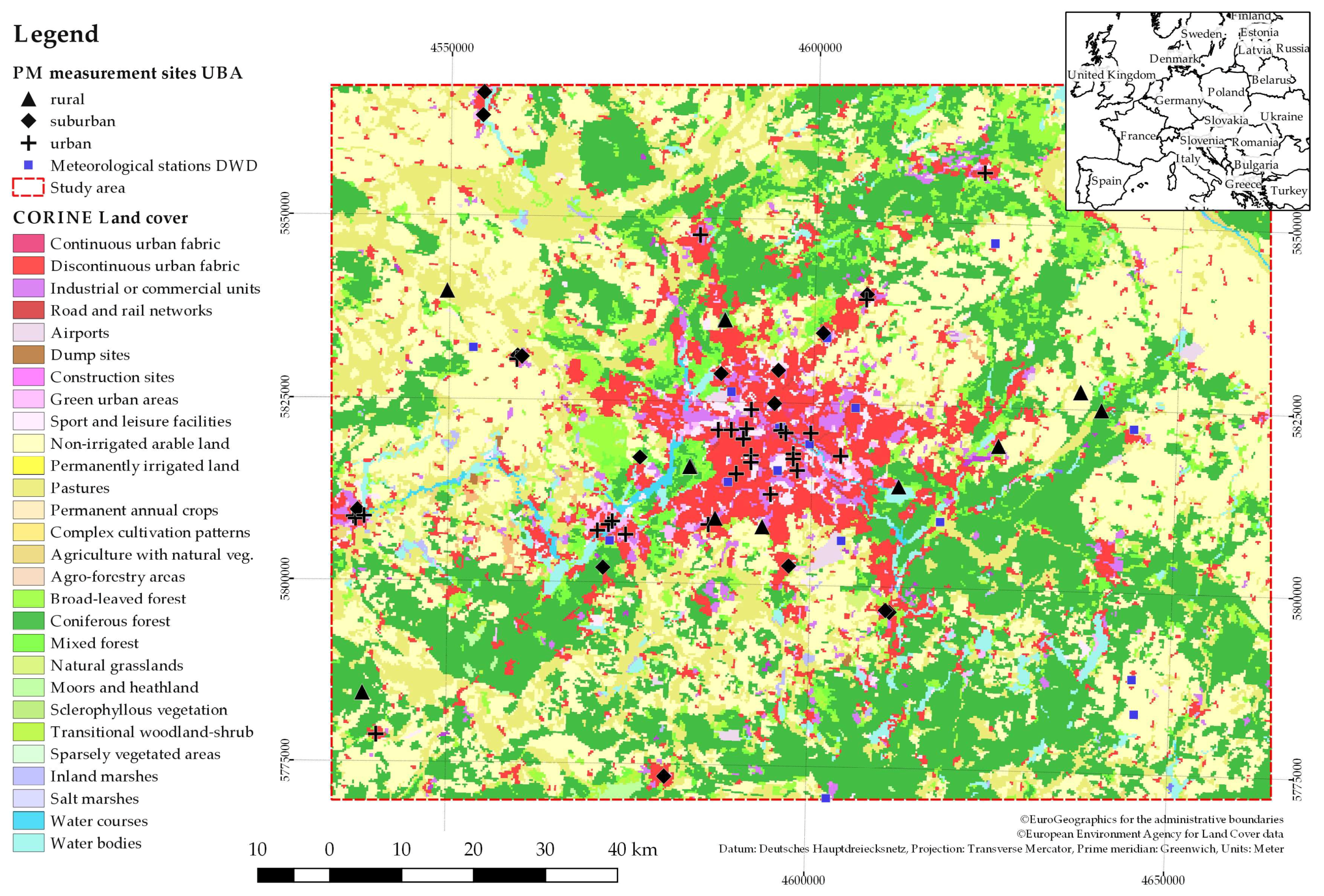
2.1. Study Domain

The study focuses on a rectangular area (∼12,000 km${}^2$) around the cities of Berlin and Potsdam in northeastern Germany. A relatively small area was chosen to properly quantify and interpret influencing factors of the relationship between AOD and PM10. The area is dominated by the cities in its center and is surrounded by agricultural land and large vegetated areas to the north and south (see Figure 1). A great number of PM10 measurements in the city area and its surroundings are available. The area is mainly characterized by continental climate with only sparse, episodic maritime influence when advection of air masses from northern and northwestern directions occurs. Thus, the area is suitable for studying the influence of wind direction to discriminate between these regimes.

Local PM10 sources dominate in the region, with traffic the major contributor [4]. Vegetated areas surrounding Berlin influence the mixture of particles in and around the urban area. The emission of Biogenic Volatile Organic Compounds (BVOCs, e.g., isoprene and monoterpenes) leads to secondary aerosol formation. Depending on the vegetation type, this effect can vary significantly; agricultural areas, for example, can have pollution levels similar to the urban background. It has been argued that particle transport from the east can markedly contribute to overall pollution levels [4,33]. In general, two different air mass regimes can be discriminated. Western air masses tend to transport lower particle concentrations, whereas continental, eastern air masses accumulate particles and thus carry elevated particle concentrations [34].

2.2. Materials

2.2.1. PM-Measurements

PM10 is analyzed in this study instead of PM2.5 due to a greater availability of data for the study region. PM10 measurements might be more adequate for the analysis, as larger particles are less easily transported and more representative of local conditions. Additionally, PM2.5 excludes the fraction of larger particles, which are nevertheless accountable for light extinction and are thus measured by the satellite. The stations are run by the German Federal Environmental Agency (UBA) and consist of hourly mean concentrations [$\mathsf{\mu }$g/m${}^3$]. PM concentrations are determined by measuring the attenuation of $\beta$-radiation by a dust-coated filter. Measurements are largely uninfluenced by ambient temperature and relative humidity. To avoid condensation, the particle inlet is heated permanently [25].

The locations of PM measurement sites and station types are shown in Figure 1. Instructions by the European Union prescribe measurement sites to be sited in such a way that micro-environment effects can be avoided. Stations can be of type background or traffic and be representative for urban, rural or suburban areas. Traffic sites are generally close to main roads or busy intersections [35]. These sites are excluded from the analysis as they are by design not representative for conditions beyond the specific traffic situation and thus the area covered by a satellite pixel. PM concentrations within the city area reach their maximum in the morning hours (∼ 7–8 a.m.) and in the evening (∼ 9–11 p.m.) [36]. Urban background sites capture the integrated contribution of all sources near the site without one particular source dominating. These stations are representative for some km${}^2$. Suburban stations need to be placed downwind (referring to the main wind direction) of emission sources and ensure a representativeness of some dozends km${}^2$. Rural background stations may not be influenced by agglomerations or industrial sites closer than five kilometers. These stations may be located in small settlements, given a representativeness of some hundred km${}^2$ [35].

2.2.2. Satellite AOD Data

High-resolution (1 × 1 km) AOD computed by application of the MAIAC technique is used [37,38,39,40]. The product is based on data from MODIS, Collection 6, aboard the Terra and Aqua satellites. The MAIAC algorithm makes use of look-up tables, explicitly taking into account surface bidirectional reflectance factors (BRF). The calculation of AOD relies on the assumption that surface BRFs remain largely constant over time, considering a time series of 16 consecutive days. This assumption might not be true in case of rapid surface changes, e.g., green-up events over bright surfaces [37,38]. To avoid these pixels, uncertainty estimates as included in the product are applied for filtering here. Pixels with an uncertainty larger 0.4 were discarded. For valid daytime AOD data used in this study, Aqua and Terra satellite overpass times range from ∼9 a.m. UTC to ∼1 p.m. UTC.

2.2.3. Meteorological Data

To represent regional-scale meteorological conditions, ERA-Interim reanalysis data generated by the ECMWF are used with a resolution of 0.125° [41]. These include BLH [m] and wind speed [m/s] in u and v direction (10 m height). Wind speed and wind direction [°] are calculated using u and v wind components. BLH data are employed as a proxy for the vertical concentration of aerosols in the lower troposphere, assuming particles are well-mixed within the boundary layer [12,42] and AOD mostly represents attenuation in the boundary layer [43]. Depending on the closest satellite overpass time, ERA-Interim data at 9 a.m. UTC, 12 noon UTC or 3 p.m. UTC are used.

Ground measurements were obtained from the DWD. One hour mean values of RH [%] measured in 2 m height are used [44]. The locations of DWD measurement sites are given in Figure 1 as blue dots. This study uses near-ground RH measurements, as these are more widely available than measurements of the vertical distribution of water vapour. Under dry conditions (RH < 55%), near-ground RH measurements show reasonable agreement with vertically resolved measurements. This might not be the case at higher RH [32].

2.3. Methods

UBA PM station coordinates are used as spatial reference, i.e., AOD pixels, ERA-Interim pixels and meteorological station data coordinates are collocated with the position of these stations. Only the nearest pixels below a threshold of 0.015° (∼1 km) distance from the PM measurement were collocated with the corresponding closest UBA station. The relatively small distance threshold was chosen to ensure that the MAIAC AOD reflects the situation in close vicinity of the UBA station. Terra/Aqua satellite overpass time is used as temporal reference for the PM10 and meteorological data, i.e., values closest to the overpass time are used. The work flow of this study is summarized in Figure 2.

For the analysis of factors influencing the relationship between AOD and PM10, this study introduces the Air Quality Rank Difference Index (AiRDI). The AiRDI allows for a direct, semi-quantitative assessment of whether AOD and PM10 agree, or whether the satellite qualitatively over- or underestimates PM10. Accordingly, situations in which these parameters are of similar magnitude can be identified systematically. The AiRDI is dimensionless and is computed for each spatially and temporally collocated AOD-PM10 data pair. First, AOD and PM10 values are sorted from lowest to highest on a monthly basis. The sorting is performed for each month individually to eliminate seasonal effects as outlined in the introduction. The sorted AOD (PM10) values are then assigned ranks corresponding to their positions on a scale from 0 to the number of AOD (PM10) observations per month (n), yielding AOD${}_{ranked}$ and PM10${}_{ranked}$. The rank of AOD (PM10) within each month is then divided by n and multiplied by 100, yielding normalized ranks greater than 0 and up to 100. Finally, the AiRDI is computed by subtracting PM10${}_{rank}$ from AOD${}_{rank}$ (see Equation (3)).

$$AO{D}_{rank}\left(month\right)=\frac{AO{D}_{ranked}}{n\left(month\right)}\ast 100$$

(1)

$$PM{10}_{rank}\left(month\right)=\frac{PM{10}_{ranked}}{n\left(month\right)}\ast 100$$

(2)

$$AiRDI\left(month\right)=AO{D}_{rank}\left(month\right)-PM{10}_{rank}\left(month\right)$$

(3)

Positive AiRDI means that AOD${}_{rank}$ is higher than PM10${}_{rank}$. In other words, the satellite observation is relatively higher than the PM10 concentration, indicating a relative overestimation of PM10 by the MAIAC AOD. The opposite is true for a negative AiRDI; in this case, lower AOD${}_{rank}$ coincide with higher PM10${}_{rank}$, indicating an underestimation of PM10 by the MAIAC AOD. In cases where the AiRDI is close to zero, AOD and PM10 are in the same range.

3. Results

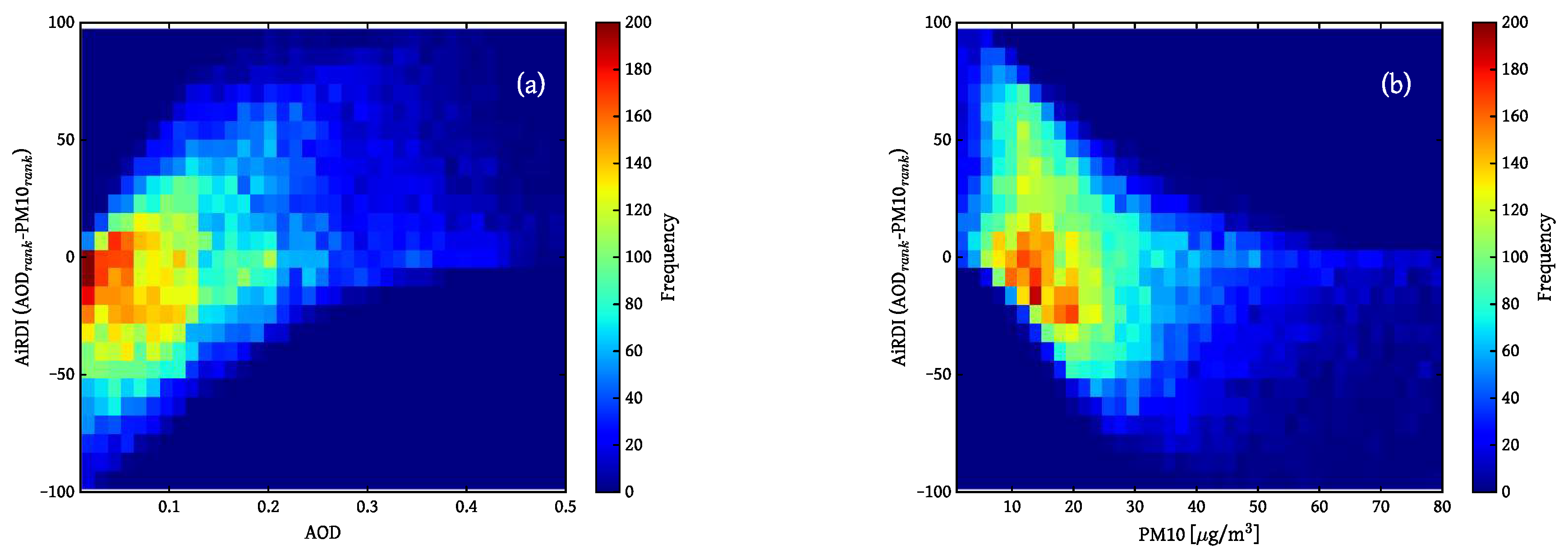
3.1. Nonlinearity of the relationship between AOD and PM10

Several studies report a robust linear correlation between daily means of AOD and PM, e.g., for the southern U.S. [10], the Po Valley in Italy [16] or selected cities worldwide [20]. In the Berlin study area, the relationship between AOD and PM10 is highly nonlinear. This is suggested by patterns shown in Figure 3a,b, which depict AiRDI in relation to AOD and PM10. A strong positive linearity would result in a slope of zero, as increasing AOD would coincide with increasing PM10, resulting in a constant AiRDI. In fact, the figures show an almost linear increase (decrease) of AiRDI for increasing AOD${}_{rank}$ (PM10${}_{rank}$). Higher (lower) AOD is likely to overestimate (underestimate) PM10 concentrations; AiRDI is more likely to be positive for high AOD, but more likely to be negative for low AOD. The pattern is inverse for the comparison of PM10 and AiRDI.

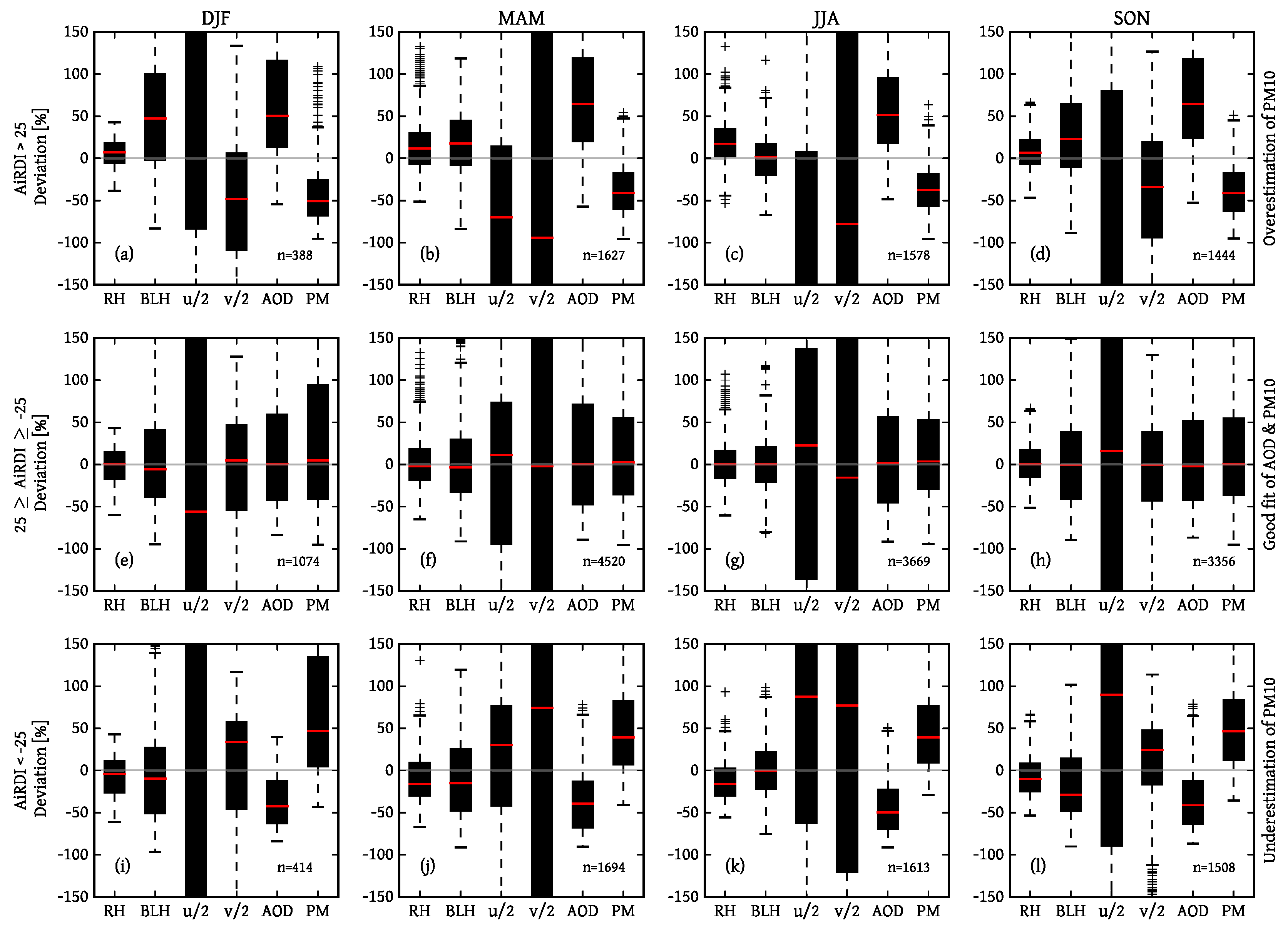
3.2. Meteorological Conditions of AOD-PM10 Agreement and Divergence

In this section, meteorological factors governing the relationship between AOD and PM10 are identified and connected to the AiRDI. An in-depth analysis concerning the role of RH and BLH is conducted. Wind speed and direction is investigated to determine the role of weather conditions and the prevailing inflow direction. AiRDI patterns related to wind are partly driven by the redistribution of RH and BLH.

To identify possible factors influencing AiRDI, data was split in positive (AiRDI > 25), negative values (AiRDI < −25) and AiRDI values close to zero (25 ≥ AiRDI ≥ −25). Subsequently, the median of each parameter for each season was calculated. Then, the relative deviation of each data point from this median for each AiRDI-class was determined, resulting in the distribution shown in Figure 4.

The class AiRDI > 25 is characterized by strong positive deviations of BLH and slightly positive RH deviations. This is consistent with what was introduced above: a higher BLH tends to decrease PM10 concentrations near ground because particles disperse within the atmospheric column, while elevated ambient RH tends to initiate hygroscopic growth, increasing AOD [10,12]. Both effects combined result in a positive AiRDI. Additionally, a high BLH might increment the number of particles distributed in the lower troposphere due to enhanced turbulence. Subsequently, AOD would also increase [13]. BLH does not show a marked deviation in summer, pointing to a decreased importance of BLH during the summer months.

Patterns of the class AiRDI < −25 display almost inverse characteristics. Here, BLH and RH show negative deviations. Negative AiRDI values result from low BLHs, which increase PM10 concentrations near ground, whereas low ambient RHs decrease the influence of hygroscopic growth. PM10 concentrations appear to have very high positive deviations in winter months, when particles are often confined to layers close to the ground [13]. The frequent occurrence of stable stratification situations along with low turbulent atmospheric exchange during stagnant synoptic situations could lead to very high particle concentrations [26].

Parameters in the class 25 ≥ AiRDI ≥ −25 do not show strong deviations of any parameter. The best agreement between AOD and PM10 is achieved when RH and BLH are near their seasonal median values.

In summary, AOD observations coinciding with high (low) ambient RH and high (low) BLH have a higher probability to cause an overestimation (underestimation) of PM10. Patterns are largely constant throughout the year. Wind speed and direction also play an important role. But like RH and BLH, the relationship is complex and is treated in more detail in the following sections.

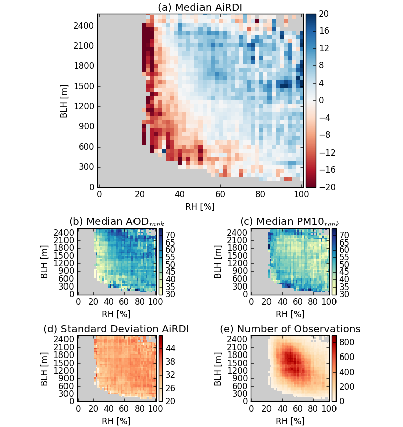
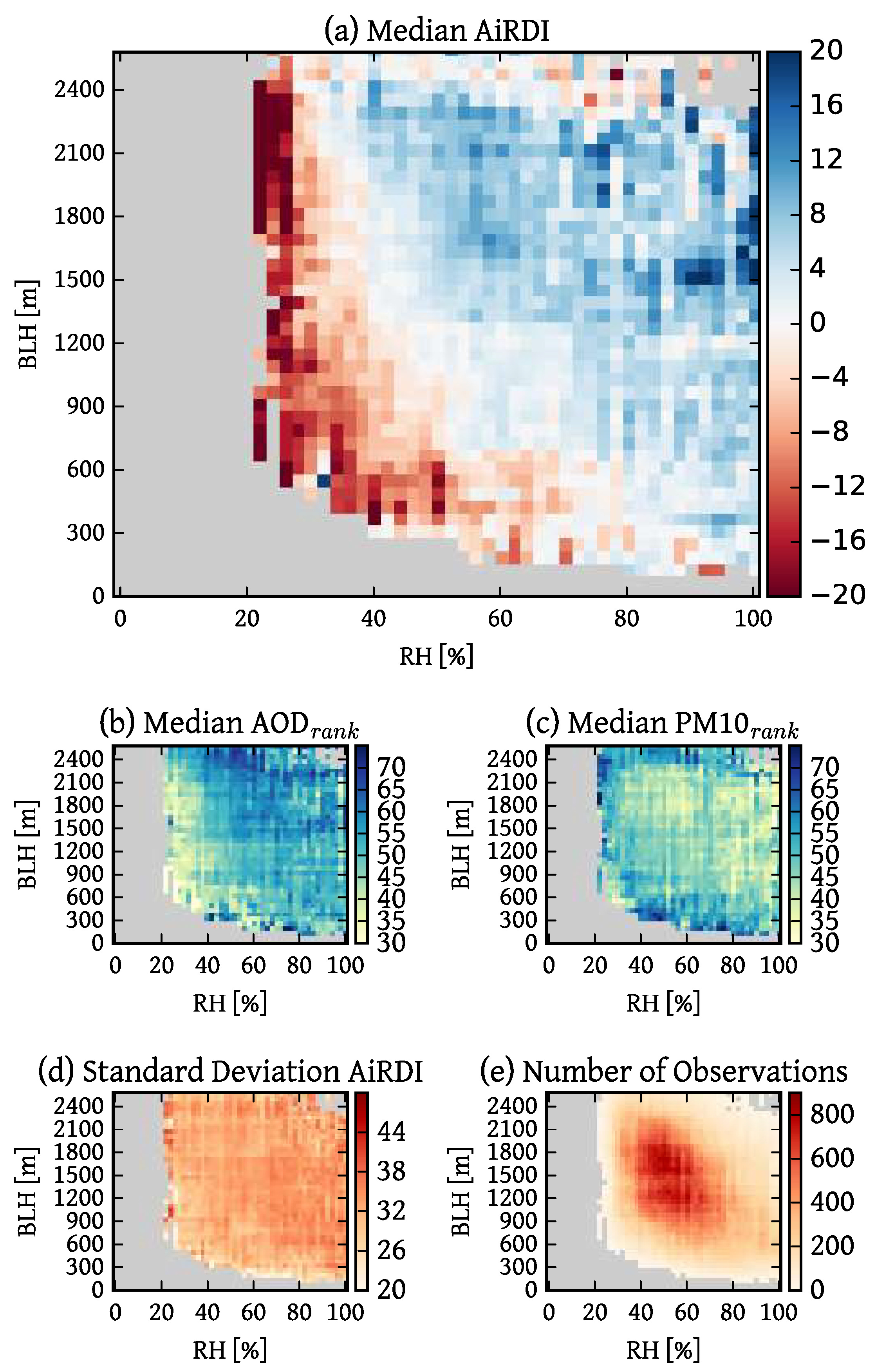
3.3. The Role of RH and BLH

This section quantifies the interconnected effects of RH and BLH on the relationship between AOD and PM10. To this end, a multivariate analysis was conducted using ranges of RH and BLH. These were related to AOD${}_{rank}$, PM10${}_{rank}$ and AiRDI.

Three AiRDI-regimes can be discriminated in Figure 5a. Low RH coinciding with low BLH leads to negative AiRDI values, relatively high RH coinciding with high BLH leads to positive AiRDI values. A curved area of near-zero AiRDI values separates negative and positive AiRDI patterns, indicating meteorological conditions where the magnitudes of AOD and PM10 match closely. The shape of this patch emphasizes the dependency of the AiRDI on both RH and BLH. With decreasing BLH, the near-zero values are shifted towards higher RH. Obviously, the effects on AiRDI of both parameters can compensate each other, leading to a AiRDI close to zero.

Figure 5b highlights the effect of hygroscopic growth on AOD, with increased RH leading to higher AOD${}_{rank}$. Furthermore, the data suggest that AOD${}_{rank}$ is positively correlated not only to RH, but also to BLH (Figure 5b). Relatively high AOD${}_{rank}$ coincides with relatively high BLH. This effect might be due to convection processes, which increase the BLH and cause particles to be lifted up into the atmosphere more easily. In these situations, the deposition of particles would be prevented and particles would remain in the atmosphere, causing the AOD to increase. Low BLH, as an indicator of low turbulence, would lead to reduced particle release and thus relatively low AOD. Additionally, when particles are confined in a shallow boundary layer, a reduced path length for satellite measurements might reduce the sensitivity to AOD [31].

PM10${}_{rank}$ is elevated for BLH < 600 m (Figure 5c) owing to limited dissipation of particles into higher atmospheric layers and subsequent accumulation of particles near the ground. At very high BLH (>2400 m), PM10${}_{rank}$ is also slightly elevated. Around 3% of all observations are related to this pattern. PM10${}_{rank}$ at these high BLH values should be interpreted with care: For mid-latitudes, BLH > 2400 m appears to be very high [45] and might not properly reflect real conditions. A weak dependence of PM10${}_{rank}$ on RH exists: PM10${}_{rank}$ decreases with increasing RH. This might be due to the fact that RH is elevated when precipitation influenced the atmosphere prior to the measurement, leading to increased RH and decreased particle concentrations due to wet deposition of particles [26]. Another possible reason might be that the influence of maritime air is overrepresented in situations with high RH. These air masses are humid and clean, i.e., carry fewer particles. Finally, this pattern could be due to measurement errors of the UBA PM sites caused by condensation on the particle inlet of the PM sensors, despite the heating of the sensor inlet. This way, fewer particles would reach the sensor, decreasing reported particle concentrations.

When BLH is greater than 600 m, the AiRDI is mostly driven by RH. In a very moist atmosphere (RH > 90%), the median AiRDI is near zero only at very low BLH. The influence of hygroscopic growth on AOD is apparent when AiRDI approaches positive values. In these situations, AOD is increased while PM10 remains unaffected. This effect can be seen from about RH > 40%, depending on BLH. Previous studies report that hygroscopic growth starts at RH ∼ 50% [46].

Results presented in this section partly contradict earlier studies, which identify situations with low BLH and low RH as favorable [20]. Figure 5a suggests that a very low BLH tends to cause an underestimation of PM10 concentrations by the satellite (negative AiRDI). RH and BLH clearly have an interconnected influence on the relationship between AOD and PM10, which emphasizes the need to examine both parameters simultaneously. Generally, AOD and PM10 match best when the atmosphere is relatively dry (40% < RH ≤ 70%) and BLH is at medium levels (600–1200 m). High ambient RH, on the other hand, can be compensated by a low BLH, leading to a good agreement of AOD and PM10. RH measurements used in this study only capture near-ground ambient RH. Nevertheless, Figure 5a suggests that near-ground RH has a large influence on the relationship between AOD and PM10.

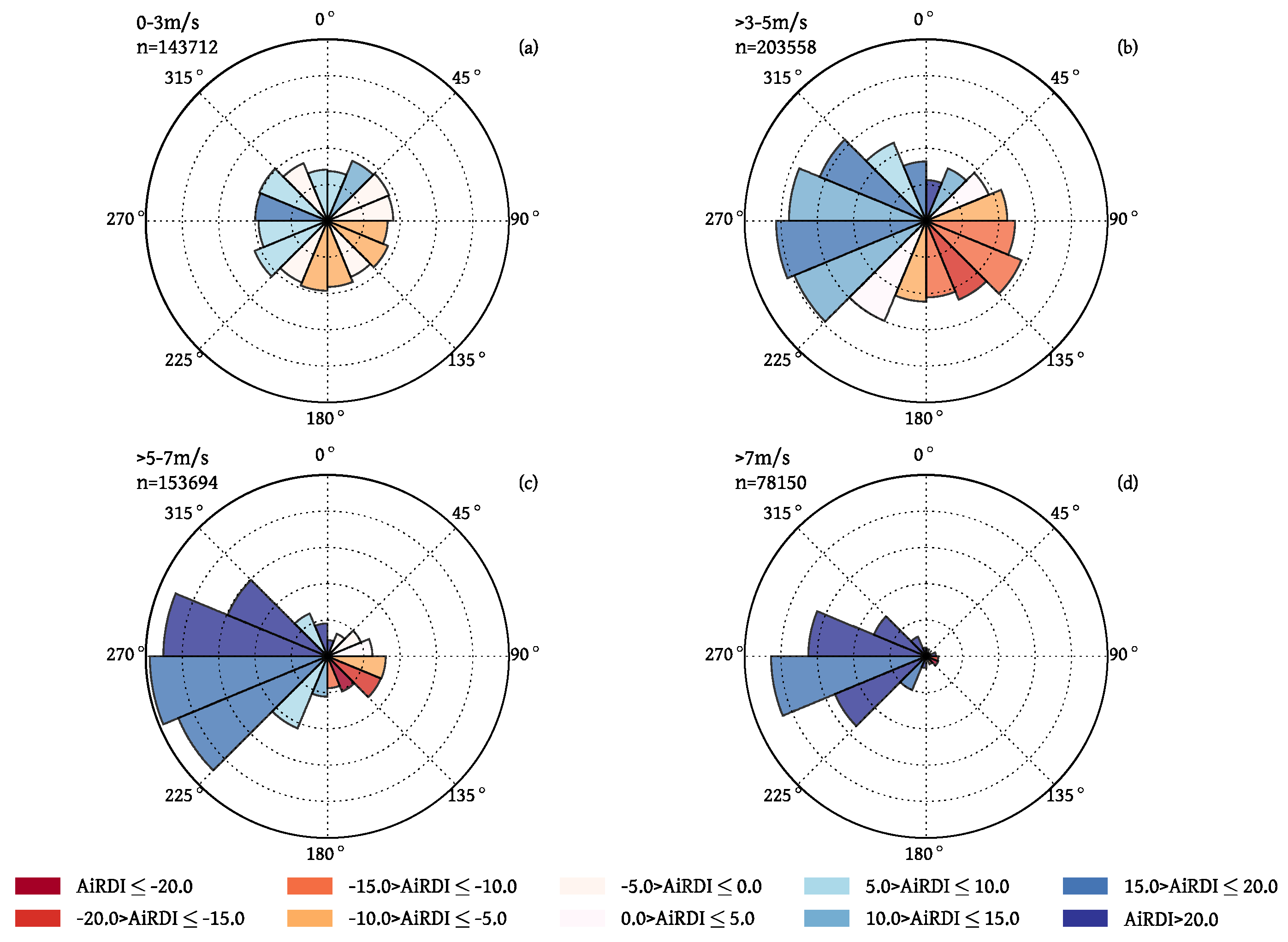
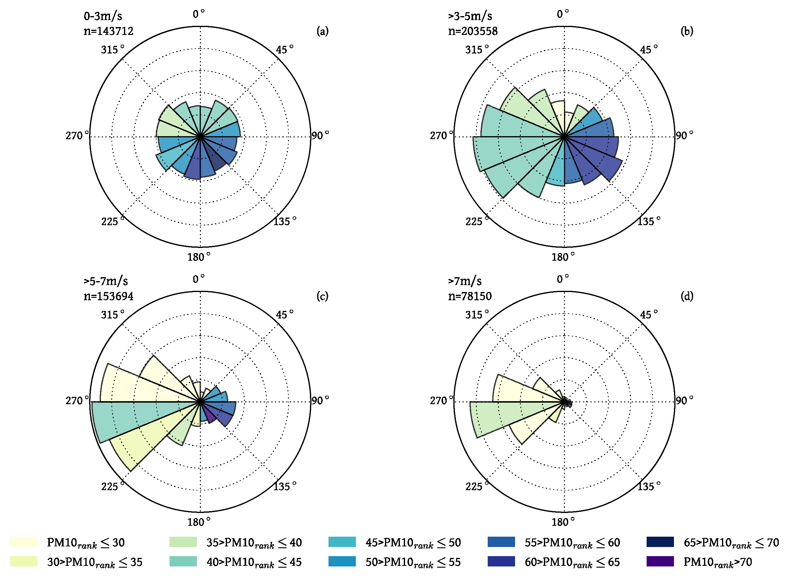
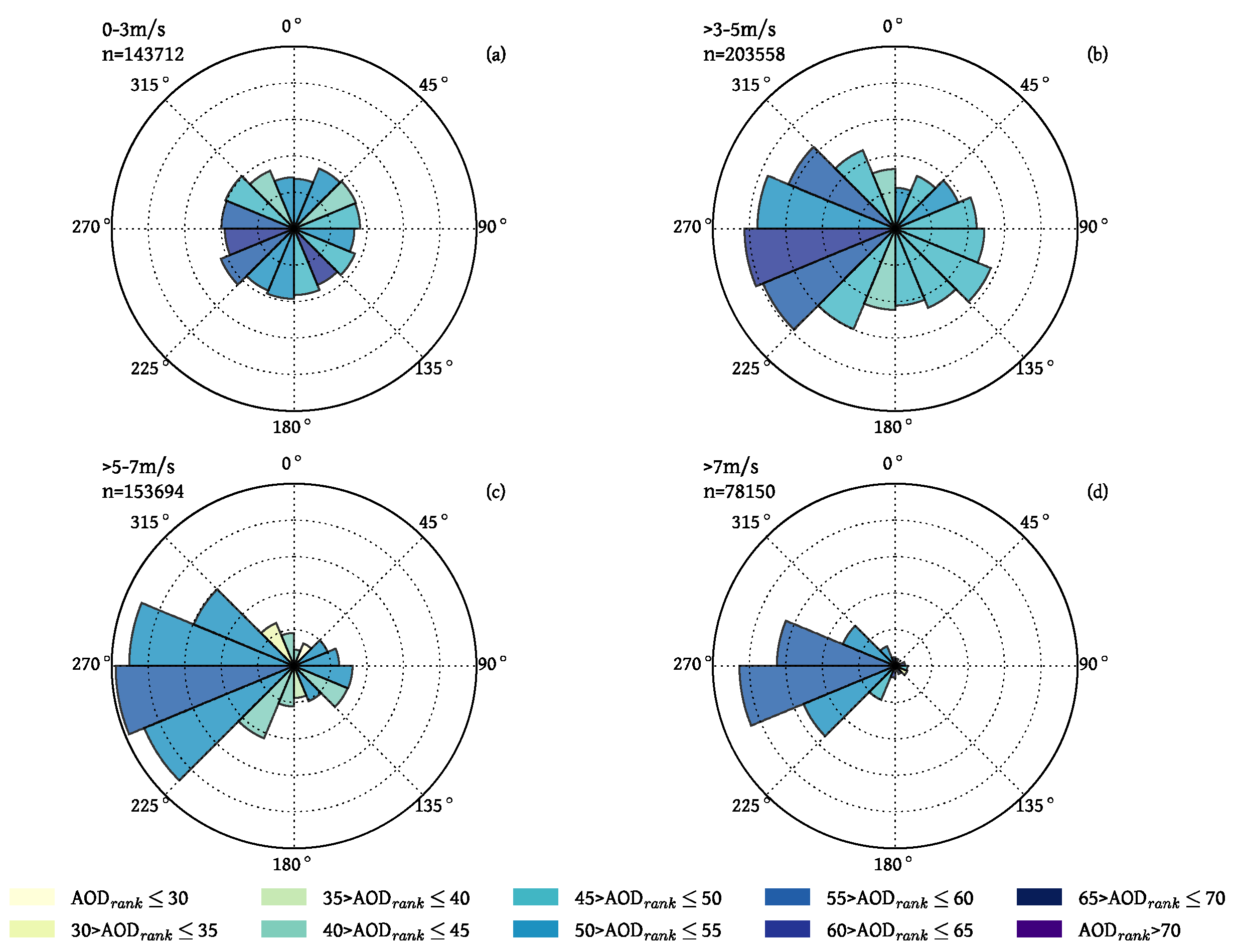
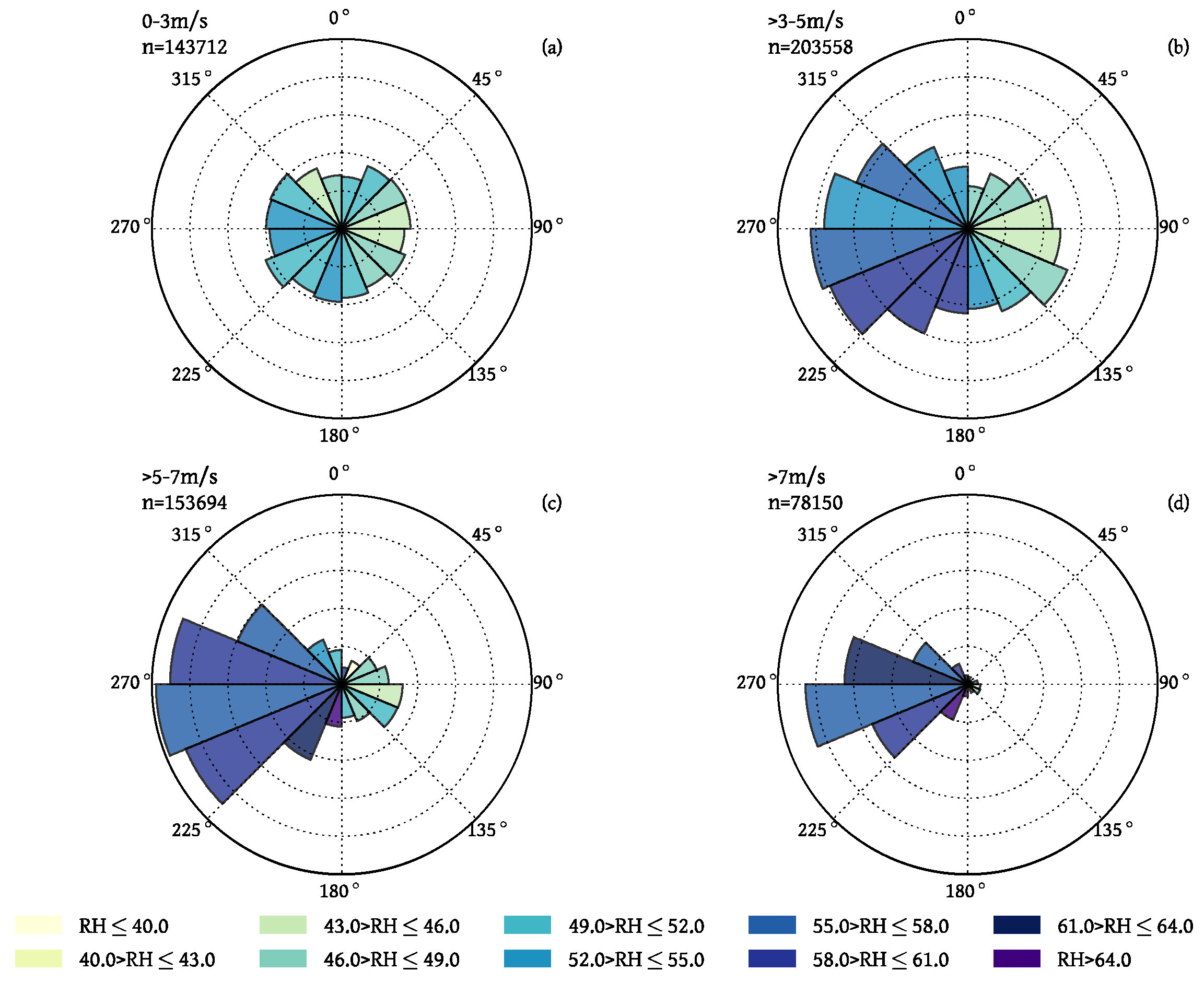
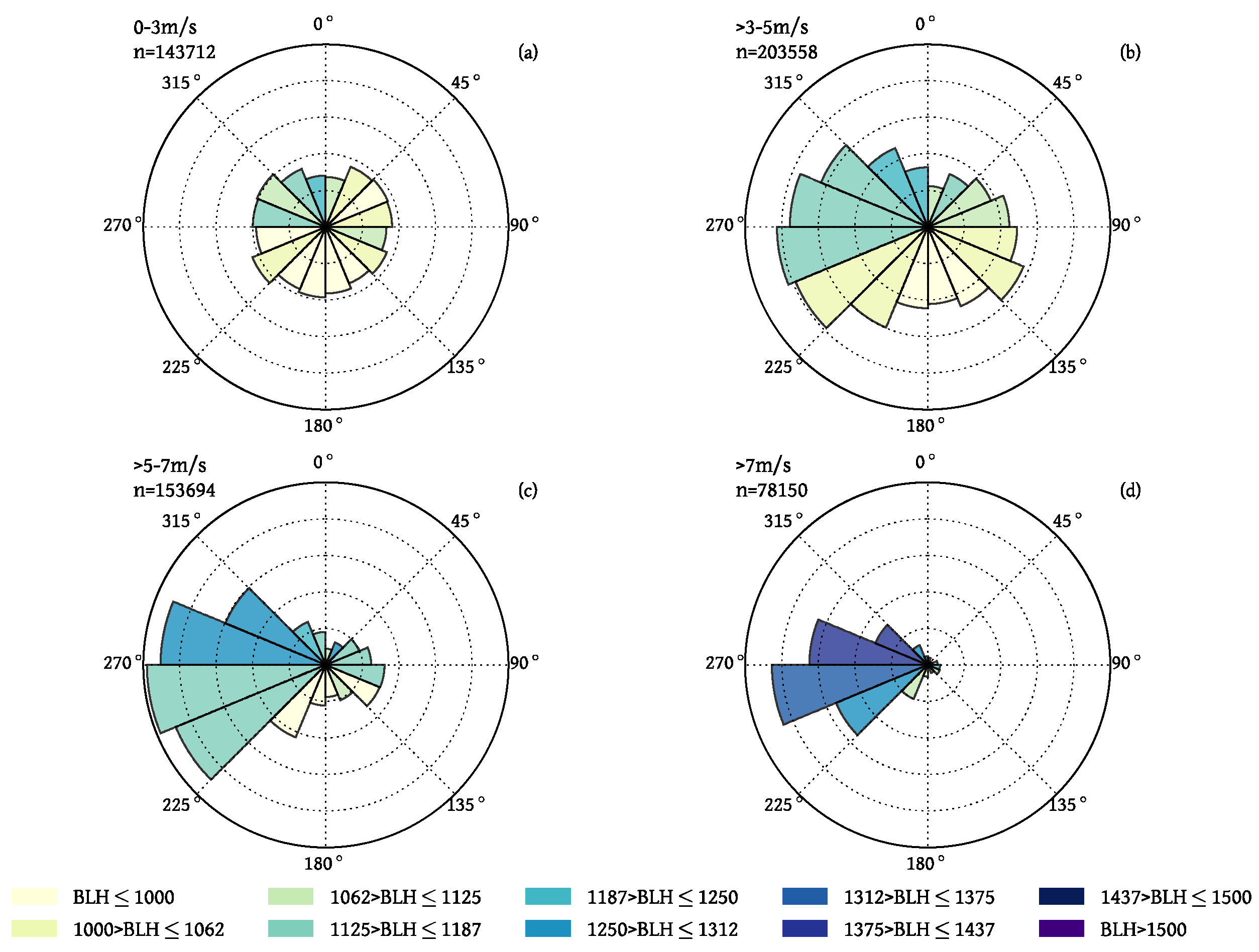
3.4. The Role of Wind Direction and Wind Speed

In this section, patterns of AiRDI, AOD${}_{rank}$ and PM10${}_{rank}$ in relation to large scale patterns of wind speed and wind direction are analyzed and connected to results of previous chapters. Patterns of wind speed and direction give hints on particle origins. Knowledge on the direction of origin of air masses, for example, helps characterize particle species and concentrations [23,24]. Wind speeds help to distinguish between the dominance of local sources or particles originating further away.

To distinguish between the effects of wind speed and direction, wind speed data are split in four classes 0–3 m/s, >3–5 m/s, >5–7 m/s and >7 m/s. The resulting polar plots are comprised of 16 wind direction classes with a range of 22.5${}^{\circ }$, starting from 0${}^{\circ }$. Each class is colored with the corresponding median AiRDI value, computed of all associated AOD${}_{rank}$ and PM10${}_{rank}$ that appear in the corresponding class. Radii of the polar bars indicate the frequency of occurrence.

A clear AiRDI pattern can be identified in Figure 6. Air masses from northwestern or western direction tend to cause a positive AiRDI, while air masses from the east and south-east tend to coincide with negative AiRDI values. This pattern is most distinctive for wind speed classes >3–5 m/s and >5–7 m/s. For lower wind speeds (0–3 m/s), the pattern is less clearly defined. This is likely due to the dominance of local particle sources, superimposing the effects of large-scale air mass transports. Results suggest that satellite AOD tends to overestimate particle concentrations near the ground when strong northwestern or western winds prevail, whereas an underestimation occurs when eastern and southeastern winds dominate. There is a higher chance of AiRDI close to zero at lower wind speeds, as local emissions can be captured more easily by both ground stations and the satellite.

PM10${}_{rank}$ (Figure 7a–d) is generally highest during conditions with low wind speeds (0–3 m/s). This is not surprising, as transport of pollutants takes place less effectively and particles from local sources inside the urban area of Berlin accumulate in the atmosphere. Additionally, dry deposition of particles might take place more effectively, as particles reach the surface more easily due to decreased vertical winds. This might lead to increased PM10 concentrations at the measurement sites. Winds from eastern directions show elevated PM10${}_{rank}$, indicating advection of continental air masses with high particle numbers near the ground. Air masses from the west, possibly of maritime origin, tend to be cleaner than continental air, because particles are scavenged by wet deposition [23,26]. At higher wind speeds, this pattern is most distinct.

Generally, patterns for AOD${}_{rank}$ are less pronounced (Figure 8a–d). In contrast to PM10${}_{rank}$, AOD${}_{rank}$ is slightly elevated when high wind speeds occur from the west . The inverse pattern of AOD${}_{rank}$ versus PM10${}_{rank}$ in terms of wind speed and wind direction demonstrates that satellite derived AOD is not suited for directly deriving ground-based PM10 in all situations.

Several explanations for these observations are possible. Advection of western air masses transports higher amounts of moisture to the Berlin study area, indicated by higher values of RH in Figure 9. Increased availability of moisture in the atmosphere could promote particle water uptake and cause hygroscopic swelling of particles. Increased particle sizes would lead to rising AOD${}_{rank}$ but not affect PM10${}_{rank}$, which ultimately leads to positive AiRDI. Eastern winds, on the other hand, transport continental air masses with a potentially larger particle loading [4,33]. This might increase PM10 concentrations.

A further possible explanation might be the varying hygroscopicity of particles carried by different air masses. Western air masses are thought to carry a higher amount of hydrophilic particles (e.g., sea salts) which tend to be more prone to hygroscopic growth due to more effective water uptake [23,24,47]. The opposite might be true for air masses from eastern and northeastern origins carrying anthropogenic and industrial aerosols. For the measurement station Melpitz, located around 130 km south of Berlin, it was found that the scattering enhancement of particles was lowest when air masses were advected from the east and northeast [23,34]. Thus, these particles are less likely to increase the AOD by hygroscopic growth [23,24]. Finally, eastern wind directions might indicate a stable atmospheric situation with lower BLH (see Figure 10), causing pollution levels to increase near the ground [12,18]. As can be seen in Figure 10, advection of air masses from the west at higher wind speeds tends to increase BLH.

In summary, advection of western air masses tends to increase RH and BLH, coinciding with slightly elevated AOD${}_{rank}$ and low PM10${}_{rank}$. Eastern and southeastern air masses tend to show lower RH and BLH, coinciding with slightly decreased AOD${}_{rank}$ and elevated PM10${}_{rank}$. These patterns are generally more pronounced for higher wind speeds, whereas dependence on wind direction decreases with lower wind speeds. To conclude, the following statements summarize the findings of this chapter:

• Western air masses with higher wind speeds establish a relatively high probability that the satellite AOD overestimates PM10.
• The opposite is true for eastern direction of origin. In these cases, a higher probability of the satellite AOD underestimating PM10 levels exists.
• Differences in RH and BLH patterns seem to be the main drivers behind the dependence of AiRDI on wind direction besides the transport of pollutants and varying hygroscopicity of particles.
• Agreement between AOD and PM10 is more likely to occur when wind speeds are low.

4. Conclusions

Information on RH, BLH, wind direction and speed proved to be of importance, driving the relationship between AOD and PM10. Generally, AOD serves as a good proxy for PM10 concentrations near ground when a very dry atmosphere (30% < RH ≤ 50%) coincides with a high BLH (>1200 m), when moderate ambient RH (50–80%) coincides with moderate BLH (600–1200 m) or when humid conditions (RH > 80%) coincide with a shallow BLH (<600 m). In case of a dry atmosphere, AOD is not influenced by hygroscopic growth and thus relatively low. This can be compensated by low PM10 levels, which appear more frequently in situations with a high BLH. When ambient RH is high, satellite-derived AOD tends to overestimate street-level PM10 concentrations. This effect can be compensated by a low BLH, which tends to increase PM10 levels near the ground. In combination, these effects can lead to an AiRDI close to zero, indicating a good match of satellite-retrieved AOD and ground-based PM10 measurements. When moderate RH and BLH prevail, AOD is only marginally affected by hygroscopic growth due to limited availability of moisture, and particle concentrations in the boundary layer seem to agree well with particle concentrations near the ground. These results suggest that it might be misleading to examine RH and BLH separately.

In terms of wind speed and wind direction, it was found that situations with prevailing western direction of origin have a higher probability to cause a positive AiRDI, whereas winds from the east tend to cause a negative AiRDI. The AiRDI is more likely to be near-zero in situations with low wind speeds.

The AiRDI proved to be a useful approach to a perform semi-quantitative comparison of the parameters AOD and PM10 and to better understand their interactions with surrounding meteorological conditions. Knowledge of the effect of these conditions can help future approaches to derive high-quality PM estimates based on AOD. The AiRDI approach can be generalized for application in other study areas. Still, this study did not account for some sources of uncertainties, for example effects of cloud contamination or aerosol layers above the BLH [32,48]. Future analyses could further focus on the role of different aerosol species or the role of precipitation events on the relationship between AOD and PM.

References

1. Wichmann, H.; Spix, C.; Tuch, T.; Wölke, G.; Peters, A.; Heinrich, J.; Kreyling, W.; Heyder, J. Daily mortality and fine and ultrafine particles in Erfurt, Germany part I: role of particle number and particle mass. Res. Rep. (Health Eff. Inst.) 2000, 98, 5–86. [Google Scholar]
2. Lim, S.S.; Vos, T.; Flaxman, A.D.; Danaei, G.; Shibuya, K.; Adair-Rohani, H.; Amann, M.; Anderson, H.R.; Andrews, K.G.; Aryee, M.; et al. A comparative risk assessment of burden of disease and injury attributable to 67 risk factors and risk factor clusters in 21 regions, 1990–2010: A systematic analysis for the Global Burden of Disease Study 2010. Lancet 2012, 380, 2224–2260. [Google Scholar] [CrossRef]
3. Samoli, E.; Stafoggia, M.; Rodopoulou, S.; Ostro, B.; Declercq, C.; Alessandrini, E.; Díaz, J.; Karanasiou, A.; Kelessis, A.G.; Tertre, A.L.; et al. Associations between fine and coarse particles and mortality in Mediterranean cities: Results from the MED-PARTICLES project. Environ. Health Perspect. 2013, 121, 932–938. [Google Scholar] [CrossRef] [PubMed]
4. Bonn, B.; Von Schneidemesser, E.; Andrich, D.; Quedenau, J.; Gerwig, H.; Lüdecke, A.; Kura, J.; Pietsch, A.; Ehlers, C.; Klemp, D.; et al. BAERLIN2014—The influence of land surface types on and the horizontal heterogeneity of air pollutant levels in Berlin. Atmos. Chem. Phys. 2016, 16, 7785–7811. [Google Scholar] [CrossRef]
5. Berlin Senate. Luftreinhalteplan 2011–2017. Available online: https://www.berlin.de/ (accessed on 24 August 2018).
6. Qadir, R.M.; Abbaszade, G.; Schnelle-Kreis, J.; Chow, J.C.; Zimmermann, R. Concentrations and source contributions of particulate organic matter before and after implementation of a low emission zone in Munich, Germany. Environ. Pollut. 2013, 175, 158–167. [Google Scholar] [CrossRef] [PubMed]
7. Ellison, R.B.; Greaves, S.P.; Hensher, D.A. Five years of London’s low emission zone: Effects on vehicle fleet composition and air quality. Transp. Res. Part D Transp. Environ. 2013, 23, 25–33. [Google Scholar] [CrossRef]
8. Wolff, H. Keep your clunker in the suburb: Low-emission zones and adoption of green vehicles. Econ. J. 2014, 124, F481–F512. [Google Scholar] [CrossRef]
9. Churkina, G.; Kuik, F.; Bonn, B.; Lauer, A.; Grote, R.; Tomiak, K.; Butler, T.M. Effect of VOC Emissions from Vegetation on Air Quality in Berlin during a Heatwave. Environ. Sci. Technol. 2017, 51, 6120–6130. [Google Scholar] [CrossRef] [PubMed]
10. Wang, J.; Christopher, S. Intercomparison between satellite-derived aerosol optical thickness and PM 2.5 mass: Implications for air quality studies. Geophys. Res. Lett. 2003, 30, 2095. [Google Scholar] [CrossRef]
11. Engel-Cox, J.A.; Holloman, C.H.; Coutant, B.W.; Hoff, R.M. Qualitative and quantitative evaluation of MODIS satellite sensor data for regional and urban scale air quality. Atmos. Environ. 2004, 38, 2495–2509. [Google Scholar] [CrossRef]
12. Gupta, P.; Christopher, S.A. Particulate matter air quality assessment using integrated surface, satellite, and meteorological products: Multiple regression approach. J. Geophys. Res. 2009, 114, D14205. [Google Scholar] [CrossRef]
13. Barnaba, F.; Putaud, J.P.; Gruening, C.; Dell’Acqua, A.; Dos Santos, S. Annual cycle in co-located in situ, total-column, and height-resolved aerosol observations in the Po Valley (Italy): Implications for ground-level particulate matter mass concentration estimation from remote sensing. J. Geophys. Res. Atmos. 2010, 115, 1–22. [Google Scholar] [CrossRef]
14. Kloog, I.; Koutrakis, P.; Coull, B.A.; Lee, H.J.; Schwartz, J. Assessing temporally and spatially resolved PM2.5 exposures for epidemiological studies using satellite aerosol optical depth measurements. Atmos. Environ. 2011, 45, 6267–6275. [Google Scholar] [CrossRef]
15. Chudnovsky, A.; Tang, C.; Lyapustin, A.; Wang, Y.; Schwartz, J.; Koutrakis, P. A critical assessment of high-resolution aerosol optical depth retrievals for fine particulate matter predictions. Atmos. Chem. Phys. 2013, 13, 10907–10917. [Google Scholar] [CrossRef] [Green Version]
16. Arvani, B.; Pierce, R.B.; Lyapustin, A.I.; Wang, Y.; Ghermandi, G.; Teggi, S. Seasonal monitoring and estimation of regional aerosol distribution over Po valley, northern Italy, using a high-resolution MAIAC product. Atmos. Environ. 2016, 141, 106–121. [Google Scholar] [CrossRef]
17. Koelemeijer, R.B.; Homan, C.D.; Matthijsen, J. Comparison of spatial and temporal variations of aerosol optical thickness and particulate matter over Europe. Atmos. Environ. 2006, 40, 5304–5315. [Google Scholar] [CrossRef]
18. Geiß, A.; Wiegner, M.; Bonn, B.; Schäfer, K.; Forkel, R.; Von Schneidemesser, E.; Münkel, C.; Lok Chan, K.; Nothard, R. Mixing layer height as an indicator for urban air quality? Atmos. Meas. Tech. 2017, 10, 2969–2988. [Google Scholar] [CrossRef] [Green Version]
19. Van Donkelaar, A.; Martin, R.V.; Park, R.J. Estimating ground-level PM2.5 using aerosol optical depth determined from satellite remote sensing. J. Geophys. Res. Atmos. 2006, 111, 1–10. [Google Scholar] [CrossRef]
20. Gupta, P.; Christopher, S.; Wang, J.; Gehrig, R.; Lee, Y.; Kumar, N. Satellite remote sensing of particulate matter and air quality assessment over global cities. Atmos. Environ. 2006, 40, 5880–5892. [Google Scholar] [CrossRef]
21. Boyouk, N.; Léon, J.F.; Delbarre, H.; Podvin, T.; Deroo, C. Impact of the mixing boundary layer on the relationship between PM2.5 and aerosol optical thickness. Atmos. Environ. 2010, 44, 271–277. [Google Scholar] [CrossRef]
22. Wang, J.; Martin, S.T. Satellite characterization of urban aerosols: Importance of including hygroscopicity and mixing state in the retrieval algorithms. J. Geophys. Res. Atmos. 2007, 112, 1–18. [Google Scholar] [CrossRef]
23. Zieger, P.; Fierz-Schmidhauser, R.; Weingartner, E.; Baltensperger, U. Effects of relative humidity on aerosol light scattering: Results from different European sites. Atmos. Chem. Phys. 2013, 13, 10609–10631. [Google Scholar] [CrossRef]
24. Titos, G.; Jefferson, A.; Sheridan, P.J.; Andrews, E.; Lyamani, H.; Alados-Arboledas, L.; Ogren, J.A. Aerosol light-scattering enhancement due to water uptake during the TCAP campaign. Atmos. Chem. Phys. 2014, 14, 7031–7043. [Google Scholar] [CrossRef] [Green Version]
25. Umweltbundesamt. Qualitätssicherungshandbuch des UBA-Messnetzes; Technical Report; Federal Environment Agency: Berlin, Germany, 2004. [Google Scholar]
26. Rost, J.; Holst, T.; Sahn, E.; Klingner, M.; Anke, K.; Ahrens, D.; Mayer, H. Variability of PM10 concentrations dependent on meteorological conditions. Int. J. Environ. Pollut. 2009, 36, 3–18. [Google Scholar] [CrossRef]
27. Levy, J.I.; Hanna, S.R. Spatial and temporal variability in urban fine particulate matter concentrations. Environ. Pollut. 2011, 159, 2009–2015. [Google Scholar] [CrossRef] [PubMed]
28. Chudnovsky, A.; Lyapustin, A.; Wang, Y.; Tang, C.; Schwartz, J.; Koutrakis, P. High resolution aerosol data from MODIS satellite for urban air quality studies. Cent. Eur. J. Geosci. 2013, 6, 17–26. [Google Scholar] [CrossRef]
29. Stafoggia, M.; Schwartz, J.; Badaloni, C.; Bellander, T.; Alessandrini, E.; Cattani, G.; de’ Donato, F.; Gaeta, A.; Leone, G.; Lyapustin, A.; et al. Estimation of daily PM10 concentrations in Italy (2006–2012) using finely resolved satellite data, land use variables and meteorology. Environ. Int. 2017, 99, 234–244. [Google Scholar] [CrossRef] [PubMed]
30. Zheng, C.; Zhao, C.; Zhu, Y.; Wang, Y.; Shi, X.; Wu, X.; Chen, T.; Wu, F.; Qiu, Y. Analysis of Influential Factors for the Relationship between PM2.5 and AOD in Beijing. Atmos. Chem. Phys. Discuss. 2017, 1–57. [Google Scholar] [CrossRef]
31. Gupta, P.; Christopher, S.A. Particulate matter air quality assessment using integrated surface, satellite, and meteorological products: 2. A neural network approach. J. Geophys. Res. 2009, 114, D20205. [Google Scholar] [CrossRef]
32. Crumeyrolle, S.; Chen, G.; Ziemba, L.; Beyersdorf, A.; Thornhill, L.; Winstead, E.; Moore, R.H.; Shook, M.A.; Hudgins, C.; Anderson, B.E. Factors that influence surface PM2.5values inferred from satellite observations: Perspective gained for the US Baltimore-Washington metropolitan area during DISCOVER-AQ. Atmos. Chem. Phys. 2014, 14, 2139–2153. [Google Scholar] [CrossRef] [Green Version]
33. Kerschbaumer, A. On the Aerosol Budget over Berlin. Ph.D. Thesis, Free University, Berlin, Germany, 2007. [Google Scholar]
34. Zieger, P.; Fierz-Schmidhauser, R.; Poulain, L.; Müller, T.; Birmili, W.; Spindler, G.; Wiedensohler, A.; Baltensperger, U.; Weingartner, E. Influence of water uptake on the aerosol particle light scattering coefficients of the Central European aerosol. Tellus B Chem. Phys. Meteorol. 2014, 66. [Google Scholar] [CrossRef] [Green Version]
35. EU. Directive 2008/50/EC of the European Parliament and of the Council of 21 May 2008 on ambient air quality and cleaner air for Europe. Off. J. Eur. Communities 2008, 152, 1–43. Available online: https://www.eea.europa.eu/policy-documents/directive-2008-50-ec-of (accessed on 24 August 2018).
36. Von Schneidemesser, E.; Bonn, B.; Butler, T.M.; Ehlers, C.; Gerwig, H.; Hakola, H.; Hellén, H.; Kerschbaumer, A.; Klemp, D.; Kofahl, C.; et al. BAERLIN2014-stationary measurements and source apportionment at an urban background station in Berlin, Germany. Atmos. Chem. Phys. 2018, 18, 8621–8645. [Google Scholar] [CrossRef]
37. Lyapustin, A.; Martonchik, J.; Wang, Y.; Laszlo, I.; Korkin, S. Multiangle implementation of atmospheric correction (MAIAC): 1. Radiative transfer basis and look-up tables. J. Geophys. Res. Atmos. 2011, 116. [Google Scholar] [CrossRef] [Green Version]
38. Lyapustin, A.; Wang, Y.; Laszlo, I.; Kahn, R.; Korkin, S.; Remer, L.; Levy, R.; Reid, J.S. Multiangle implementation of atmospheric correction (MAIAC): 2. Aerosol algorithm. J. Geophys. Res. Atmos. 2011, 116, 1–15. [Google Scholar] [CrossRef]
39. Lyapustin, A.I.; Wang, Y.; Laszlo, I.; Hilker, T.; Hall, F.G.; Sellers, P.J.; Tucker, C.J.; Korkin, S.V. Multi-angle implementation of atmospheric correction for MODIS (MAIAC): 3. Atmospheric correction. Remote Sens. Environ. 2012, 127, 385–393. [Google Scholar] [CrossRef]
40. Lyapustin, A.; Wang, Y.; Korkin, S.; Huang, D. MODIS Collection 6 MAIAC Algorithm. Atmos. Meas. Tech. Discuss. 2018, 1–50. [Google Scholar] [CrossRef]
41. Dee, D.P.; Uppala, S.M.; Simmons, A.J.; Berrisford, P.; Poli, P.; Kobayashi, S.; Andrae, U.; Balmaseda, M.A.; Balsamo, G.; Bauer, P.; et al. The ERA-Interim reanalysis: Configuration and performance of the data assimilation system. Q. J. R. Meteorol. Soc. 2011, 137, 553–597. [Google Scholar] [CrossRef]
42. Ansmann, A.; Althausen, D.; Wandinger, U.; Franke, K.; Müller, D.; Wagner, F.; Heintzenberg, J. Vertical profiling of the Indian aerosol plume with six-wavelength lidar during INDOEX: A first case study. Geophys. Res. Lett. 2000, 27, 963–966. [Google Scholar] [CrossRef] [Green Version]
43. Schäfer, K.; Harbusch, A.; Emeis, S.; Koepke, P.; Wiegner, M. Correlation of aerosol mass near the ground with aerosol optical depth during two seasons in Munich. Atmos. Environ. 2008, 42, 4036–4046. [Google Scholar] [CrossRef]
44. DWD Climate Data Center (CDC). Historical Hourly Station Observations of 2m Air Temperature and Humidity. 2016. Available online: ftp://ftp-cdc.dwd.de/pub/CDC/observations_germany/climate/hourly/ (accessed on 24 August 2018).
45. Von Engeln, A.; Teixeira, J. A planetary boundary layer height climatology derived from ECMWF reanalysis data. J. Clim. 2013, 26, 6575–6590. [Google Scholar] [CrossRef]
46. Lee, J.; Kim, Y. Spectroscopic measurement of horizontal atmospheric extinction and its practical application. Atmos. Environ. 2007, 41, 3546–3555. [Google Scholar] [CrossRef]
47. Granados-Muñoz, M.J.; Navas-Guzmán, F.; Bravo-Aranda, J.A.; Guerrero-Rascado, J.L.; Lyamani, H.; Valenzuela, A.; Titos, G.; Fernandez-Galvez, J.; Alados-Arboledas, L. Hygroscopic growth of atmospheric aerosol particles based on active remote sensing and radiosounding measurements: Selected cases in southeastern Spain. Atmos. Meas. Tech. 2015, 8, 705–718. [Google Scholar] [CrossRef] [Green Version]
48. Bourgeois, Q.; Ekman, A.M.L.; Renard, J.b.; Krejci, R.; Devasthale, A.; Bender, F.A.; Riipinen, I.; Berthet, G.; Tackett, J.L. How much of the global aerosol optical depth is found in the boundary layer and free troposphere? Atmos. Chem. Phys. 2018, 18, 7709–7720. [Google Scholar] [CrossRef]
Figure 1. Geographical extent of the study area. Different land cover classes are colored, positions of meteorological stations and PM10-measurement sites are indicated.
Remotesensing 10 01353 g001
Figure 2. Overview of the work flow of this study. Methods are shown in curved boxes, inputs and outputs in rectangular boxes.
Remotesensing 10 01353 g002
Figure 3. 2D-histograms of AiRDI, AOD r a n k (a) and AiRDI, PM10 r a n k (b). The frequency of occurrence of associated data pairs is color-coded.
Remotesensing 10 01353 g003
Figure 4. Determination of factors influencing AiRDI including relative humidity (RH), boundary layer height (BLH), wind velocity in u and v direction (u/2,v/2), aerosol optical depth (AOD) and PM10 (PM) . Data are split on a seasonal basis and divided in positive (ad), negative values (eh) and AiRDI values close to zero (il). Winter months are denoted as DJF, spring months as MAM, summer months as JJA, fall months as SON. Box plots show the relative deviation of each parameter observation to the seasonal mean. Deviations for u and v were multiplied by a factor of 0.5 to prevent a distortion of the y-axes. The box plots extend from the lower to the upper quartile value, with a red line at the median. Whiskers show the range with outliers marked as short, horizontal black lines. The number of observations for each class is denoted as n.
Remotesensing 10 01353 g004
Figure 5. (a) Relationship between AiRDI (AOD r a n k − PM10 r a n k ), RH and BLH. BLH is gridded in steps of 60 m, RH in steps of 2%, each grid cell represents the median AiRDI. (b) Relationship between AOD r a n k , RH and BLH, same grouping of RH and BLH as (a). (c) Relationship between PM10 r a n k , RH and BLH, same grouping of RH and BLH as (a). (d) Standard deviation of AiRDI for each class, same grouping of RH and BLH as (a). (e) Number of observations for each grid cell, same grouping of RH and BLH as (a).
Remotesensing 10 01353 g005
Figure 6. Relationship between the AiRDI (AOD r a n k − PM10 r a n k ), wind direction and wind speed for the study area. Figures (ad) represent a wind speed class as shown on the upper left of each panel. Polar bars enclose a wind direction class, each 22.5 in range. Colors indicate the mean AiRDI for each polar bar, the radius of each bar indicates the frequency of occurrence.
Remotesensing 10 01353 g006
Figure 7. Relationship between PM10 r a n k , wind direction and wind speed. Setup of figures (ad) is identical to previous plot. PM10 r a n k is generally higher when continental, i.e., easterly air masses dominate.
Remotesensing 10 01353 g007
Figure 8. Relationship between AOD r a n k , wind direction and wind speed. Setup of figures (ad) is identical to previous plot.
Remotesensing 10 01353 g008
Figure 9. Relationship between RH [%], wind direction and speed. Setup of figures (ad) is identical to previous plot.
Remotesensing 10 01353 g009
Figure 10. Relationship between BLH [m], wind direction and speed. Setup of figures (ad) is identical to previous plot.
Remotesensing 10 01353 g010