Synergetic Use of Sentinel-1 and Sentinel-2 Data for Soil Moisture Mapping at Plot Scale

Abstract

This paper presents an approach for retrieval of soil moisture content (SMC) by coupling single polarization C-band synthetic aperture radar (SAR) and optical data at the plot scale in vegetated areas. The study was carried out at five different sites with dominant vegetation cover located in Kenya. In the initial stage of the process, different features are extracted from single polarization mode (VV polarization) SAR and optical data. Subsequently, proper selection of the relevant features is conducted on the extracted features. An advanced state-of-the-art machine learning regression approach, the support vector regression (SVR) technique, is used to retrieve soil moisture. This paper takes a new look at soil moisture retrieval in vegetated areas considering the needs of practical applications. In this context, we tried to work at the object level instead of the pixel level. Accordingly, a group of pixels (an image object) represents the reality of the land cover at the plot scale. Three approaches, a pixel-based approach, an object-based approach, and a combination of pixel- and object-based approaches, were used to estimate soil moisture. The results show that the combined approach outperforms the other approaches in terms of estimation accuracy (4.94% and 0.89 compared to 6.41% and 0.62 in terms of root mean square error (RMSE) and R²), flexibility on retrieving the level of soil moisture, and better quality of visual representation of the SMC map.

1. Introduction

Soil moisture content (SMC) retrieval is attracting widespread interest due to its role in regulating the water cycle and energy balance [1]. This influence makes the SMC a key variable in the fields of climatology, meteorology, hydrology, and agriculture. Unfortunately, soil moisture retrieval from direct-field measurements is time-consuming and expensive at the local scale and impractical at the global scale due to the high spatial variability of the target variable. Fortunately, remote sensing provides an alternative solution to this issue with SMC mapping over large areas with complete, repeated, and frequent coverage of the Earth’s surface.

Microwave remote sensing, both active and passive, has already revealed its potential in soil moisture retrieval independent of weather conditions. This capacity is due to the fact that microwave signals are influenced by dielectric properties (and thus the water content) of the soils [2]. It should be noted that other variables (roughness and vegetation) also affect microwave signals and this effect must be disentangled in the retrieval process of SMC from remotely sensed data. Currently, a range of sensors with different spatial and temporal resolutions are available. Passive remote sensing sensors can be used to retrieve soil moisture with a temporal resolution of 2–3 days, though because of the emission behavior of the surface, these instruments operate at a low spatial resolution (around 40 km), including the European Space Agency (ESA)’s Soil Moisture and Ocean Salinity (SMOS) mission [3,4,5] the National Aeronautics and Space Administration (NASA)’s Soil Moisture Active Passive (SMAP) mission [6,7], and ERS/WSC, ASCAT/METOP, and ASMR-E [8,9,10]. These sensors are well-suited for soil moisture estimation at regional and global scales. Although active sensors, such as ERS, RADARSAT, ASAR/ENVISAT, PALSAR/ALOS, TerraSAR-X, and Cosmo-SkyMed, are appropriate for soil moisture estimations at a high spatial resolution (better than 30 m) to provide a diagnosis suited to agricultural watershed areas, their accuracy is not as high as the passive sensors [11,12,13,14,15]. Recently, operational monitoring of soil moisture was made possible by the launch of the Sentinel-1 satellite in regular temporal coverage (6 days for Europe when both the A and B satellites are considered) together with a spatial resolution of 10 m and at no cost to the users.

In the domain of SMC retrieval, various approaches have been proposed. These approaches are categorized into three main groups: physical-based, empirical-based, and change-detection-based. Each of these methodologies reveal its specific capabilities in retrieving soil moisture values. In summary, physical-based models provide an explanation of the interactions between microwave electromagnetic radiation and the Earth’s surface. They allow for a simulation of diverse experimental scenarios in terms of sensor configurations (wavelength, polarization, incidence angle) and soil parameters (surface roughness, soil dielectric constant, vegetation cover) [16,17]. Oh, Dubois, and integral equation models (IEMs) are among the most widely used models in inversion procedures [18,19,20,21]. However, several studies have mentioned a poor agreement between measured radar signals and those predicted by the models [22,23,24]. This is a vital characteristic for guaranteeing generality and for avoiding dependency in the study area and sensor configurations, which are the main property of empirical-based methods. Although robust and accurate results can be achieved for studied areas by empirical-based methods [15,25,26], change-detection-based methods are another widely addressed technique in the literature. The main idea behind this approach is that variation in surface roughness and natural vegetation cover happens at a much longer time scale than that of surface soil moisture. Using multi-temporal data, we can relate the changes in the backscattering signal to variation in SMC with minimizing the effect of vegetation and roughness [27].

In recent years, there has been growing interest in multi-sensor fusion for retrieving soil moisture. Synthetic aperture radar (SAR) and optic data fusion is one of the most widely used approaches [28,29,30,31]. The integration of data acquired by optical sensors and SAR data may provide useful information for reducing ambiguity due to the presence of vegetation. Another possible approach is the integration of active and passive microwave data that could help to retrieve soil moisture at a higher accuracy [32,33]. The SMAP mission has been designed based on this assumption.

In another perspective, since active and passive sensors provide an SMC map at large and low scales, respectively, previous works have focused on down and upscaling to retrieve soil moisture at the intermediate scale [34,35,36,37]. A major defect of this method is reliance on mathematical techniques only to reproduce soil moisture maps at the intermediate scale without considering the reality in the field. Also, after the SMAP radar failure, NASA focused on Sentinel-1 as the replacement for SMAP radar [38]. Although SMAP was supposed to gather radiometer and radar data simultaneously and use the radar to turn 30-km-per-pixel radiometer imagery into a sharper image in which one pixel represented 9 kilometers, soil moisture retrieval at the plot scale using Sentinel-1 instead of using the default 10-m-per-pixel could better fill this gap.

The underlying motivation for this study is the development of an SMC retrieval algorithm to be used in operational missions. Many projects require an SMC map with a retrieval scale that is different from that which is provided with the operating sensors. Lower-resolution soil moisture information is required for applications related to natural disasters, such as flooding or land-slides (early warning), but also in the agricultural sector to increase irrigation and fertilization efficiency. Due to this fact, a considerable interest has been shown in downscaling and upscaling methods in recent years [35,39,40,41,42]. In this study, the synergy of single-polarized C-band Sentinel-1 and optical Sentinel-2 data was used to retrieve soil moisture at the plot scale in vegetated areas. Few researchers have addressed the issue of soil moisture retrieval at the plot scale in vegetated areas [43]. In this context, we tried to work at the object level instead of the pixel level by applying object-based image analysis (OBIA). This means that instead of working on a regular-sized pixel, we work on a group of pixels with similar properties (an image object). The grouping of neighboring pixels into image objects based on similar properties results in minimization of the SAR speckle noise. Object-based image analysis enables us to produce the most relevant objects to a soil moisture parameter with selection of the most relevant features and import them into the segmentation process. As described below, there are some limitations to adopting this approach with the available data. To resolve this issue, we propose an approach derived from the strengths of both the pixel- and object-based methods. In the proposed approach, the training phase is performed at the pixel level while the retrieval phase is carried out at the object level. We believe that a significant advantage is provided by using this combined approach. In this method, the radar and optical measurements can be effectively combined to derive soil moisture estimates at the plot scale with acceptable accuracy and intermediate resolution (the resolution between active and passive sensors). Furthermore, the OBIA procedure permits us to extract image objects with various sizes in an operational project so that fields of any magnitude can be identified and retrieved. This viewpoint will enable us to have a degree of flexibility on the retrieval scale. This approach seems to better meet the practical application requirements. It should be noted that the radar data used in this study was C-band data from the Sentinel-1 satellite and in the single polarization mode (VV polarization). Previous studies have shown that VV polarization is not the most relevant polarization in the soil moisture retrieval process [29,44,45]. Also, the studied areas are under vegetation cover and the C band is not considered the best band for exploiting in areas with vegetation cover. Therefore, the scenario used in this study is considered as a challenging scenario in terms of sensor characteristics and the characteristics of the study area.

Hence, the novelties addressed in the paper are as follows.

(1)

A test of a specific strategy for soil moisture retrieval in the areas with dominant vegetation cover using single polarized (VV) C-band Sentinel-1 and optical Sentinel-2 data.

(2)

A derivation of soil moisture at the plot scale with acceptable accuracy.

(3)

Having flexibility in the retrieval scale based on user needs.

This article is organized as follows: Section 2 introduces the study area on which our analysis is focused and describes the adopted dataset. The major steps of the proposed algorithm for soil moisture retrieval are explained in Section 3. Section 4 is devoted to the detailed description of the proposed algorithm and presentation of the results and discussion. Finally, Section 5 draws the conclusion from the study.

2. Area of Interest and Available Satellite Data Sets

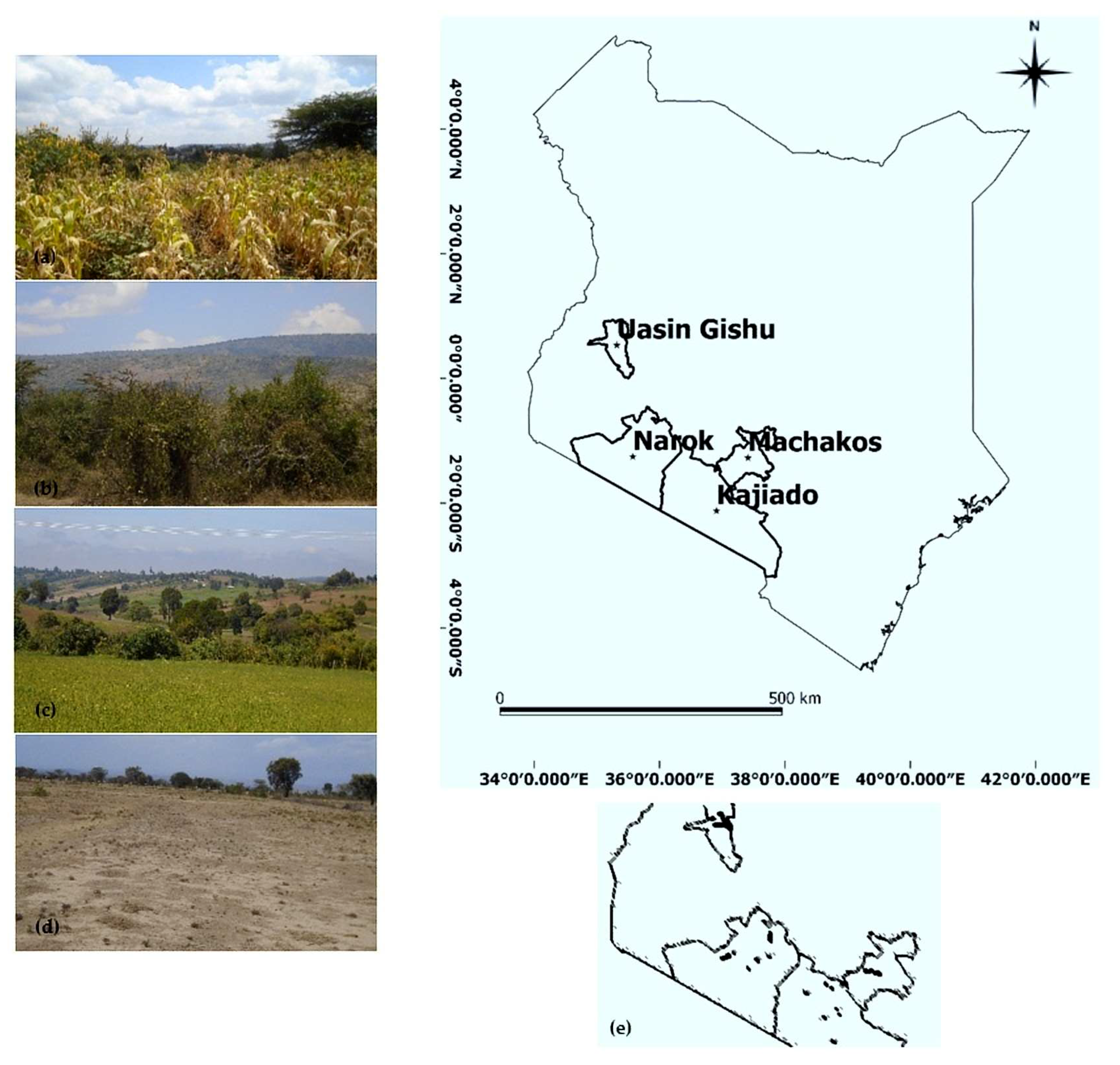
2.1. Study Area

Four different study areas, including Uasin Gishu, Machakos, Narok, and Kajiado County in Kenya, were selected for the collection of the field data. Data were collected during six field campaigns: Uasin Gishu County was visited twice and all other areas were visited once. The collected data were used for training and validation of the Support Vector Regression soil moisture retrieval algorithm. A total of 164 spatially different samples, with 2–4 replicates each, were collected. A short description of the areas visited is given below (Figure 1). The majority of the measurements are in the domain between 0 and 20% SMC. However, even with fewer samples, the domain between 20 and 50% is fully covered as well. This means that samples for the entire expected range of SMC values were collected, which is crucial since this data is also used for the training of the support vector regression retrieval model. Land use is composed of cropland (55, 72, 49, and 2%), shrubland (25, 8, 21, and 89%), forestland (11, 3, 1, and 3%), riverine (1, 0, 1, and 0%), grassland (3, 14, 23, and 5%), waterbody (0, 1, 2, and 0%), wetland (2, 0, 0, and 0%), bareland (1, 0, 2, and 0%), and settlement (2, 2, 1, and 1%) for Uasin Gishu, Machakos, Narok, and Kajiado county, respectively. It should be noted that most of the in situ data were measured within cropland, shrubland, and grassland fields. We considered four types of soil coverage, including bare soil and soil with sparse, moderate, and dense vegetation cover. The canopy height was also divided into five categories, including less than 10 cm, 10–25 cm, 25–50 cm, 50–75 cm, and greater than 75 cm.

Uasin Gishu County is a highland plateau with altitudes falling gently from 2700 m to about 1500 m above sea level. The topography is higher to the east and declines gently towards the western border. The soils, which are comprised of red loam soils, red clay soils, brown clay soils, and brown loam soils, mainly support maize, sunflower, wheat, pyrethrum, potato, and barley farming. They also support livestock rearing and forestry. Uasin Gishu experiences high and reliable rainfall, which is evenly distributed throughout the year. The average rainfall ranges between 624.9 mm and 1560.4 mm with two distinct peaks occurring between March and September and May and August. Dry spells occur between November and February. The temperatures range between 7 degrees Celsius and 29 degrees Celsius. Generally, these conditions are favorable for livestock keeping and crop and fish farming.

Machakos County is an administrative County in the eastern part of Kenya. The prevailing local climate is semi-arid and the landscape is hilly, rising from an altitude of 1000 to 1600 m above sea level. Only 31 percent of land in the high- and medium-potential area is under production, which represents only 5 percent of the land in the county. Arid and semi-arid lands (ASALs) represent 84 percent of the land, which remains largely underutilized. The high population growth rate has led to a continuous decrease in average farm sizes [46]. The average farm size under small-scale farming is 0.756 hectares while that under large-scale farming is 10 hectares.

Narok County is situated in Kenya along the Great Rift Valley. It covers an area of 17,944 km² and has a population of 850,920. The temperature range is 12 to 28 °C and the average rainfall range is 500 to 1800 mm per annum. As per the U.N. study for the Kenya Vision 2030, Narok County is marked as one of the fundamental counties for achieving an economic pillar [47]. Key contributions are in the tourism sector through the Maasai Mara and the agricultural sector through livestock farming.

Kajiado County lies at the southern edge of the former Rift Valley province, about 80 km from the Kenyan capital Nairobi. Kajiado sits on an area of 21,901 square kilometres and borders Nakuru, Nairobi, and Kiambu to the north, Narok to the west, Makueni and Machakos to the east, and Taita-Taveta and Tanzania to the south. Kajiado County is primarily semi-arid. The average annual temperature in the county is 18.9 °C. The area receives about 500 mm of rainfall annually, most of it falling in April. The month of August is usually extremely dry.

2.2. Sentinel-1 Data

Ten Sentinel-1A images were acquired between April and October 2016. The images were acquired in Interferometric Wide (IW) swath mode (a 250 km swath width at 5 m by 20 m spatial resolution) with incidence angles between 29° and 46° and using VV polarization (

Table 1. Main characteristics of the Sentinel-1 (S-1A), Sentinel-2 (S-2A), and in situ measurements used in this study in cells with two rows: S-1A (upper row), S-2A (lower row).

Site	Acquisition Date dd/mm/yy	Time UTC	Incidence Angle	Spatial Resolution (m × m)	Polarization	Number of Samples	In Situ Soil Moisture (%) [Min; Max]
Kajiado	16/08/2016 02/08/2016	15:55 07:55	38°	5 × 20 20 × 20	VV + VH	27	[3.3; 26.8]
Machakos	31/05/2016 08/04/2016	15:47 07:55	38°	5 × 20 20 × 20	VV	7	[4.1; 43.7]
Narok	05/09/2016 25/08/2016	15:55 08:05	38°	5 × 20 20 × 20	VV	35	[3.2; 33.5]
Uasin Gishu	03/10/2016 14/10/2016	15:56 08:03	38°	5 × 20 20 × 20	VV	56	[3.8; 51.4]
Uasin Gishu	18/04/2016 08/04/2016	15:56 07:55	38°	5 × 20 20 × 20	VV	39	[5.4; 38.9]

VV, single polarization mode.

). Sentinel-1A GRD data were radiometrically calibrated in SNAP software. This is a necessary step to work with SAR data. Radiometrical calibration corrects an SAR image so that the pixel values truly represent the radar backscatter of the reflecting surface. The use of these calibration processes is made possible by the mosaicking of discrete data, which is essential in our work. It should be noted that Haji et al. have assessed the radiometric stability and quality of S-1A images for use in land surface applications [48]. The radar images were multilooked to 14.25 resolution for further data analysis. To reduce speckle noise, the refined lee filter was applied to the multilooked images. Terrain correction was performed with the Range-Doppler Terrain Correction module in the SNAP software using the SRTM 1 sec digital elevation model (DEM).

2.3. Sentinel-2 Data

Five optical images were acquired by Sentinel-2A over the study sites as close as possible to the SAR data (depending on cloud coverage) (Table 1). The processing of the Optical images included orthorectification and spatial registration according to a global reference system with subpixel accuracy. Optical images were atmospherically corrected using the Sen2Cor plugin, converting top-of-atmosphere (TOA) reflectances into top-of-canopy (TOC) reflectances [49], and georeferenced using the SRTM 1 sec DEM in the SNAP software.

2.4. In Situ Measurements

Simultaneously with the Sentinel-1A acquisitions, six field campaigns were conducted in order to collect information on the SMC. Nondestructive measurements were acquired using calibrated time domain reflectometry (TDR) probes. Soil moistures were collected over depths of 0–5 cm at the time of the satellite overpasses. A total of 164 spatially different samples were collected. For each sample, two to four measurements of soil dielectric constant at a few meters distance from each other were collected and averaged. These measurements were converted into volumetric moisture (mv) based on bulk density. The location of each in situ measurement was recorded using a global positioning system (GPS) device. During the ground campaign, the soil moisture values ranged between 3.2 and 51.4 vol. % (Table 1).

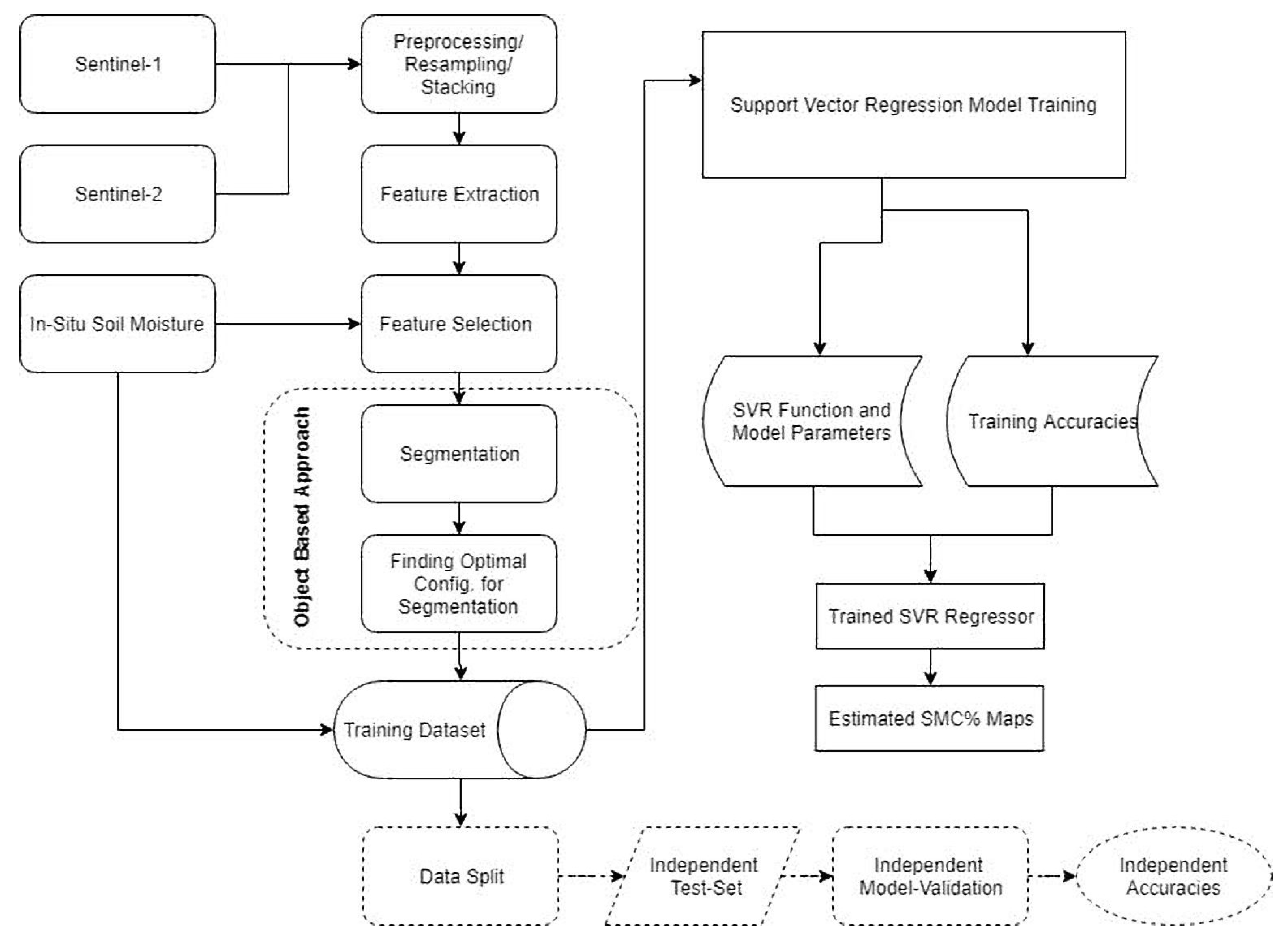
3. Soil Moisture Retrieval Algorithm

The processing chain adopted in this study for the retrieval of soil moisture is demonstrated in Figure 2. The central part of the processing chain is the retrieval algorithm. The retrieval of soil moisture is based on a machine learning approach using the support vector regression technique. SVR is a non-parametric machine learning method. It allows for the modelling of multi-dimensional and non-linear relationships between a target variable (in this case SMC) and several input features. This step enables the estimation of a desired biophysical variable from the input data. In order to achieve an efficient and robust retrieval algorithm, providing reliable and relevant inputs is a necessity. To attain this purpose, a feature extraction and selection step was developed. This procedure aims to extract and select the most appropriate features from the input data. Following these steps, soil moisture retrieval was proposed at two different levels: pixels and plots. More details on each part of the soil moisture retrieval algorithm will be given below.

3.1. Feature Extraction

Initially, we attempted to create a feature space from the Sentinel-1 and Sentinel-2 datasets. The available Sentinel-1 data for the studied region was in the single polarimetric mode while having only the VV polarization. The texture features extracted from the VV polarization were used in addition to the use of VV polarization in order to extend the radar feature space. Gray level co-occurrence (GLCM) matrix features are among the most widely used methods for textural extraction in remotely sensed images [50,51,52,53]. GLCM analysis is a second-order statistical tool generally adopted to describe texture in imagery. In this study, from a GLCM matrix, eight features are extracted: Contrast, Correlation, Dissimilarity, Entropy, Homogeneity, Mean, Standard Deviation, and Angular Second Moment.

Furthermore, due to the restriction in extracting the features from the radar data and to disentangle the vegetation effect, we attempted to utilize a broader range of the optical features. Regarding the roughness effect, we assume that information about this kind of structural contribution to the backscatter coefficient (i.e., vegetation structure and roughness) could be extracted also from the optical data. This is because there is a correlation between the type of vegetation/land cover and surface roughness—e.g., a corn-field has a different roughness than a meadow, and the corn-field will have a different roughness at different times of the year during seeding, growth, and harvest—and these could be distinguished with optical data. In this study, the optical features were extracted in three groups, namely, the soil, vegetation, and water radiometric indices. Radiometric indices are quantitative measures of features that are obtained by combining several spectral bands. The water and soil indices existing in a feature space have been considered thanks to the inherent relationship with the soil moisture parameter. In addition, the vegetation indices have been taken into account because of their dominance as a ground cover.

Table 2. Extracted texture and optical features from Sentinel-1 and Sentinel-2 imagery.

Type	Name
Radar Feature Texture Features (Extracted from VV Band)	VV Polarization GLCM Contrast GLCM Correlation GLCM Dissimilarity GLCM Entropy GLCM Homogeneity GLCM Mean GLCM Standard Dev. GLCM Angular 2nd
Optical Features	Soil Indices BI, BI2, RI, CI Vegetation Indices SAVI, NDVI, TSAVI, MSAVI, MSAVI2, DVI, RVI, PVI, IPVI, WDVI, TNDVI, GNDVI, GEMI, ARVI, NDI45, MTCI, MCARI, REIP, S2REP, IRECI, PSSRa, LAI, FCOVER Water Indices NDWI, NDWI2

GLCM, grey-level co-occurrence matrix.

exhibits all the features used in this research. More details on these radiometric indices and their formulas can be found in [54].

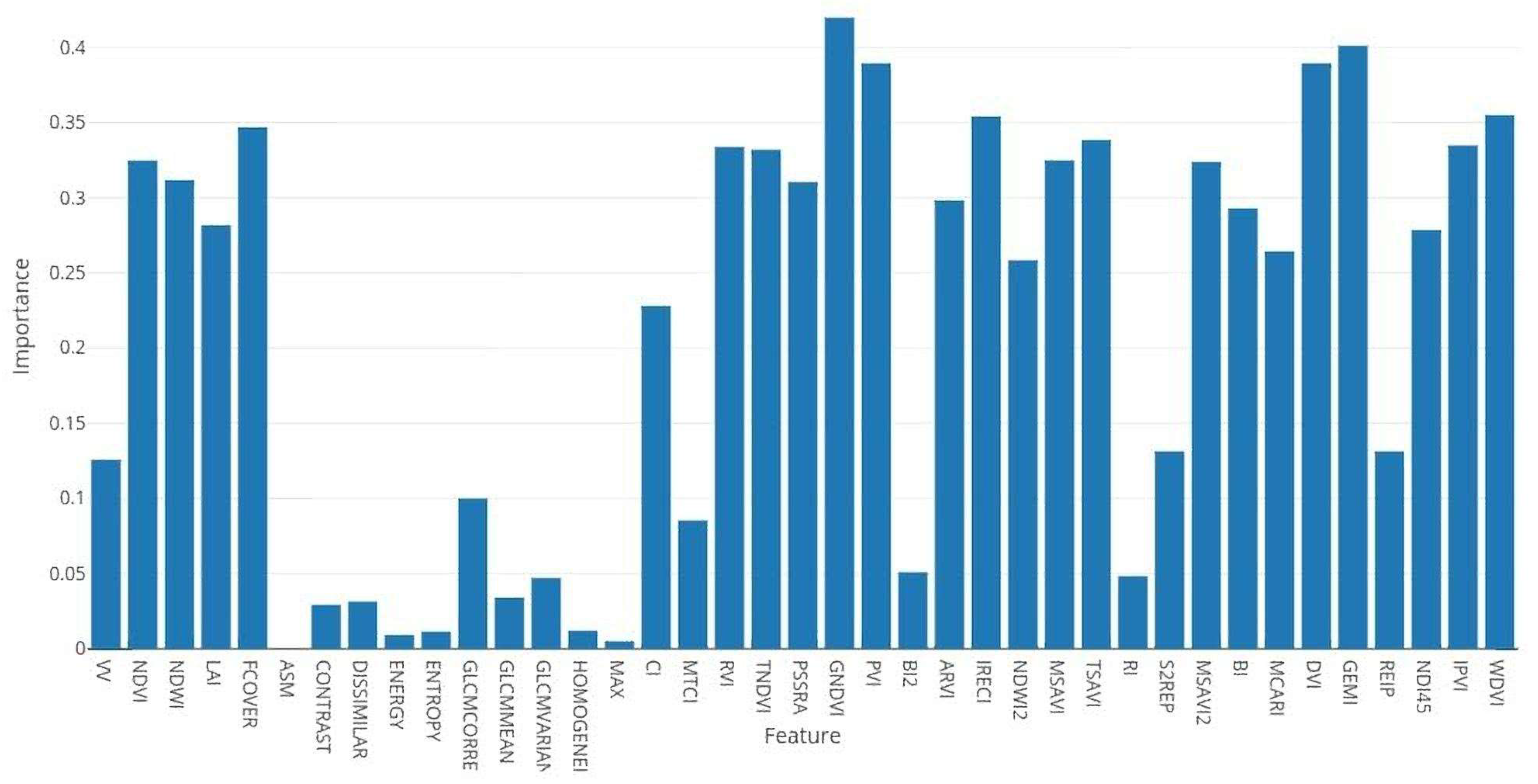
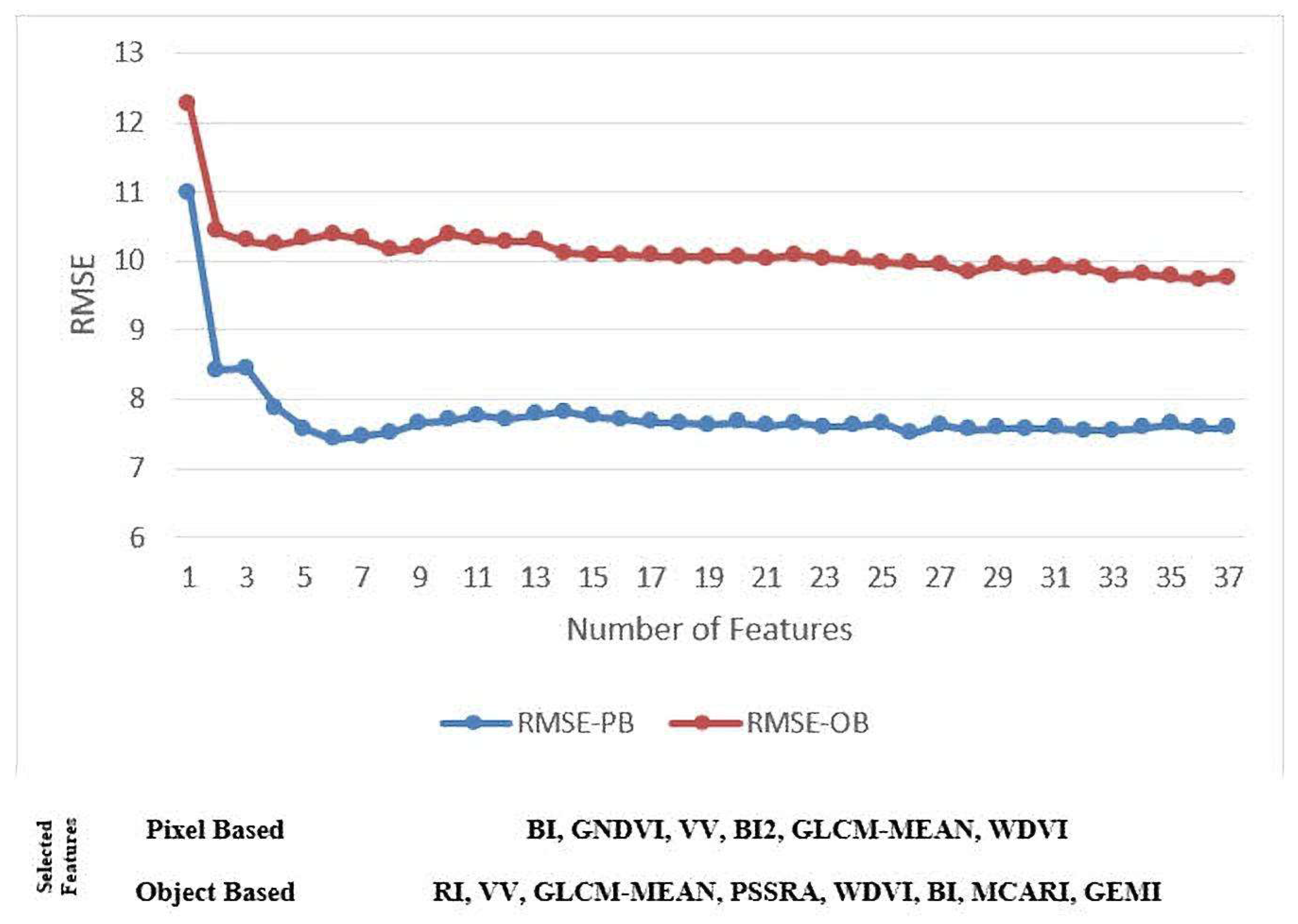
3.2. Sensivity Analysis

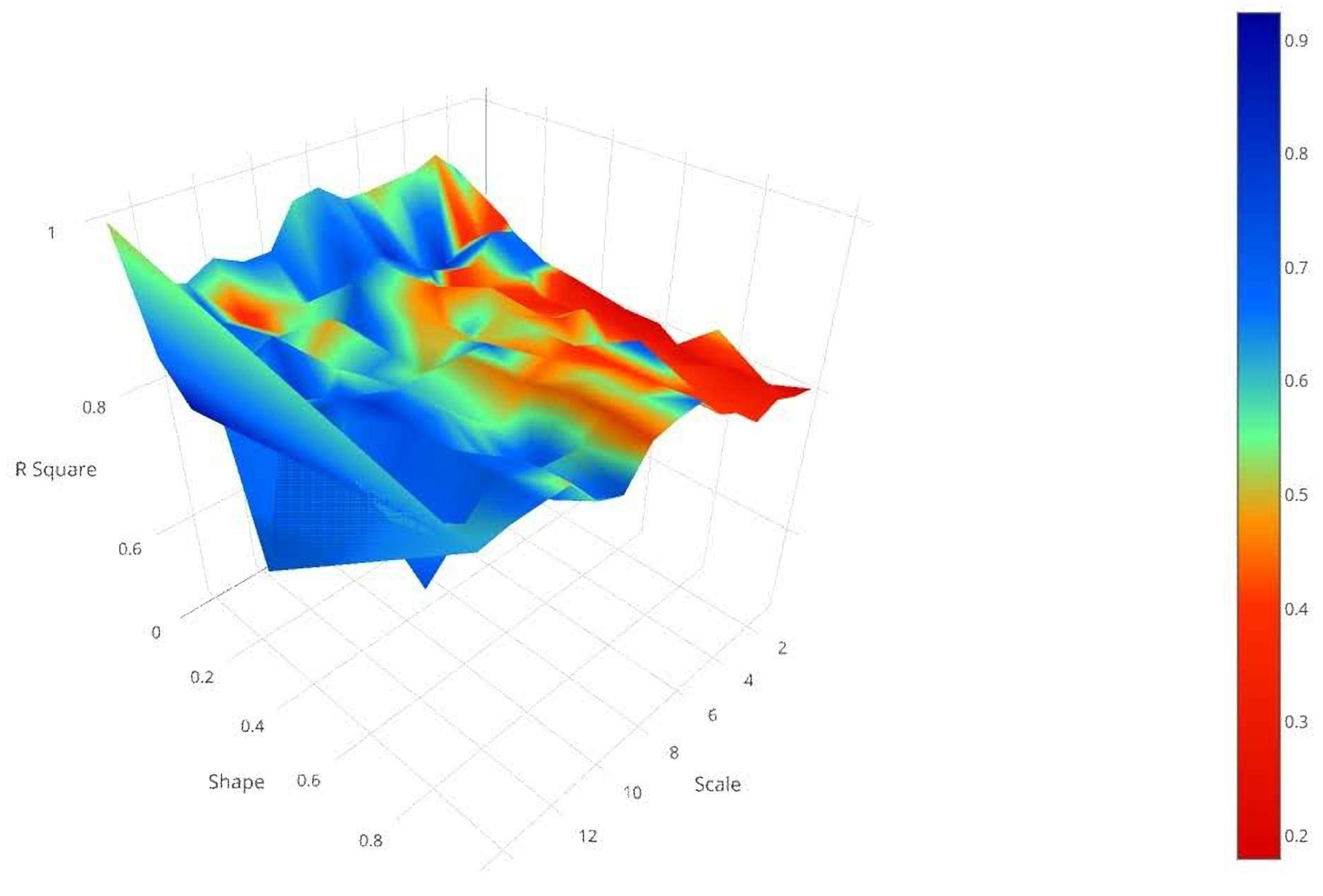
The sensitivity analysis was conducted on the extracted features from the Sentinel-1 and Sentinel-2 data in order to understand the relevance and respective weight of these features in the soil moisture retrieval approach. To fulfil this goal, the extracted features were ranked. To do so, the learning vector quantization method was used in the R software. It should be noted that in this method, the correlation of each feature with the soil moisture was measured as the degree of significance corresponding to the feature considered [55]. Figure 3 displays the output of this package. As is evident from Figure 3, the extracted optical features obtained higher significance and subsequently ranked higher, whereas the VV polarization and the texture features were found to be less important. It seems that the high correlation of the optical features, especially the vegetation indices, is due to their inherent and indirect influence on estimating the soil moisture. Further, because of the dominance of vegetation in the studied area, it seems that vegetation indices can better represent and model the existing reality.

In order to identify the best-performing subset of features in the soil moisture retrieval process, we used Random Forest-Recursive Feature Elimination (RF-RFE) as a well-known method in feature selection issues [56,57]. RF-RFE is based on the idea of repeatedly constructing a model and choosing either the best or worst performing feature, setting the feature aside, and then repeating the process with the rest of the features. A support vector machine algorithm is used on each iteration to evaluate the model. This process is applied until all features in the dataset are exhausted. Features are then ranked according to when they were eliminated. The selected features will provide the best results in terms of estimation accuracy.

As discussed below, six features have been selected among all 37 initial features for the pixel-based method. A subset with 36 features with the lowest corresponding root mean square error (RMSE) value equal to 9.73 was selected for the object-based method, although, as shown below, a subset of just 8 features yields almost comparable results.

3.3. Segmentation

Soil moisture retrieval at the plot scale has been developed based on the OBIA concept. In object-based methods, each image object is considered as a plot, which is then created at the beginning of the work using Segmentation. Segmentation was executed in the eCognition software [58] using the multiresolution segmentation algorithm (MRS).

The multiresolution segmentation algorithm primarily considers each pixel as a unique object while merging the neighboring objects through consecutive steps. Because of the merging of the two neighboring objects, the average of the homogeneity would decline; therefore, the multiresolution segmentation algorithm would seek to minimize the homogeneity decrease. In other words, an image object needs to be merged with the neighbor that results in the lowest homogeneity decrease. The segmentation procedure uses color homogeneity and shape homogeneity for object homogeneity. For a detailed review on this topic see [59,60].

Through the combining process, merging would not be achieved if the rate of the homogeneity changes for the evaluated objects exceeds the threshold defined by the user. On the other hand, if the rate is smaller than the predefined threshold, a large image object will be formed. Then, the time segmentation process will be halted so that there would be no possibility for merging two image objects exceeding the threshold rate. In this algorithm, the similarity degree of the gray value to each other in an image object is determined by the Scale Parameter. The bigger this scale parameter value is, the lesser this similarity is while the size of the objects will be bigger accordingly.

The selected scale parameter considers the color (the backscattering value for SAR data and spectral values for optical data) and shape factors simultaneously. However, in many cases the color factor is the most effective parameter in the creation process for the image objects while considering that the shape factor improves the quality of the produced objects [48]. It needs to be mentioned that the shape factor was divided into two parameters, namely smoothness and compactness.

Therefore, in the MRS algorithm, the parameters of scale, shape, and compactness have to be determined. Indeed, the amount of these parameters will exert a direct impact on the produced image objects. A determination on the optimal values for these parameters was executed in the eCognition software using a RuleSet. In this RuleSet, nested “for” loops were used, which were assigned values of 1 to 15 with an interval of 1 to the scale parameter, 0 to 1 with an interval of 0.1 to the shape parameter, and 0.1 to 0.9 with an interval of 0.1 to the compactness parameter. Finally, for each configuration, segmentation was performed and image objects are generated. The configuration obtaining the highest value of the coefficient of determination for multiple regression with field measurements of soil moisture was then considered as the optimal configuration. The optimal configuration for each region with its corresponding coefficient of determination is displayed in

Table 3. Selected configuration for each scene with the corresponding R Square.

Study Area	Segmentation Parameters
	Scale	Shape	Compactness	Max. R Square
Kajiado	9	0.1	0.4	0.92
Machakos	2	0	0.5	0.92
Narok	15	0.2	0.6	0.93
Uasin Gishu 03/10/16	11	0.2	0.4	0.74
Uasin Gishu 18/04/16	12	0.1	0.5	0.96

. Due to space constraints, Figure 4 only addresses the Machakos scene. It should be noted that there is no definite trend for defining a relationship between the values of the scale, shape, and compactness parameters in the different scenes while each scene exhibits unique behavior.

3.4. Support Vector Regression

The soil moisture retrieval algorithm is based on an advanced state-of-the-art machine learning regression method, the SVR technique. Due to its flexibility, estimation accuracy, and generalization capabilities, SVR is usually exploited in the field of geo/biophysical variable retrieval [45,61,62].

Support Vector Regression is a non-parametric machine learning method. It allows for the modelling of multidimensional and nonlinear relationships between a target variable (in this case SMC) and several input features. The application of this method for the retrieval of SMC is based on findings by [37]. The most significant gains of this method, in comparison to other retrieval strategies for our work, is its ability to handle a small training database to perform a robust retrieval. SVR overcomes this issue since it is based on a geometrical concept. SVR determines the margins of the tolerance tube around the input data. Once the margins have been determined, the mapping function can be calculated without the need for a large number of data values [63].

Due to different combinations of selected features for the pixel- and object-based approach, different SVR regressors were trained for these two cases. During the first step, model selection was carried out using a set of reference samples. Model selection refers to the process of training the SVR algorithm and tuning its free parameters, C and ε, that are kernel parameters.

These reference samples consisted of the measurements collected during the field campaigns coupled with the selected features. A window size of 3 × 3 pixels was used to compute the backscattering coefficient from the acquired Sentinel-1 images. Indeed, this window size results in a reduction of speckle noise and retains the high spatial resolution of the radar data. In the end, the prediction error for the soil moisture was evaluated using a fivefold cross-validation procedure as a good tradeoff between the stability of the results and the computational burden. To do the fivefold cross-validation, a set of 164 samples from ground measurements were divided into five equal-size subsets. Next, four of the subsets were used to train the regressor and one was retained to validate the SVR predictions.

The cross-validation procedure was then repeated five times, with each of the five subdata sets used exactly once as the validation data. The final validation result combines the five validation results. The advantage of this method over repeated random subsampling is that all observations are used for both training and validation, and each observation is used for validation exactly once [37].

In this paper, support vector regression model with the radial basis function (RBF) kernel was developed to predict soil moisture. A Gaussian RBF kernel function was chosen due to the limited computational overhead and the good performance achieved in previous analyses [49], while a grid search strategy was adopted to cover a wide spectrum of possible parameter configurations. The ranges for the grid search are [10⁻³; 10³], [10⁻⁴; 10³], and [10⁻⁴; 10] for γ (the RBF kernel width), C, and ε, respectively.

After the training/tuning phase, the independent test samples were exploited to quantitatively assess the estimation performance on reliable reference samples by means of common metrics, such as RMSE and the correlation coefficient R. With the completion of the learning phase, the trained SVR regressor was used to derive the output map of SMC. Three statistical indicators were used to evaluate the consistency between estimated parameters and measured values: the RMSE, the mean bias (Bias), and the correlation coefficient (R):

$$\mathrm{RMES}=\sqrt{\frac{1}{N}{\sum }_{i=1}^N{\left(P_i^{estimated}-P_i^{measured}\right)}^2}$$

(1)

$$\mathrm{Bias}=\frac{1}{N}{\sum }_{i=1}^N\left(P_i^{estimated}-P_i^{measured}\right)$$

(2)

$$\mathrm{R}=\frac{1}{N}{\sum }_{i=1}^N\frac{\left|P_i^{estimated}-P_i^{measured}\right|}{P_i^{measured}}$$

(3)

where P is the estimated/measured parameter and N is the number of data points.

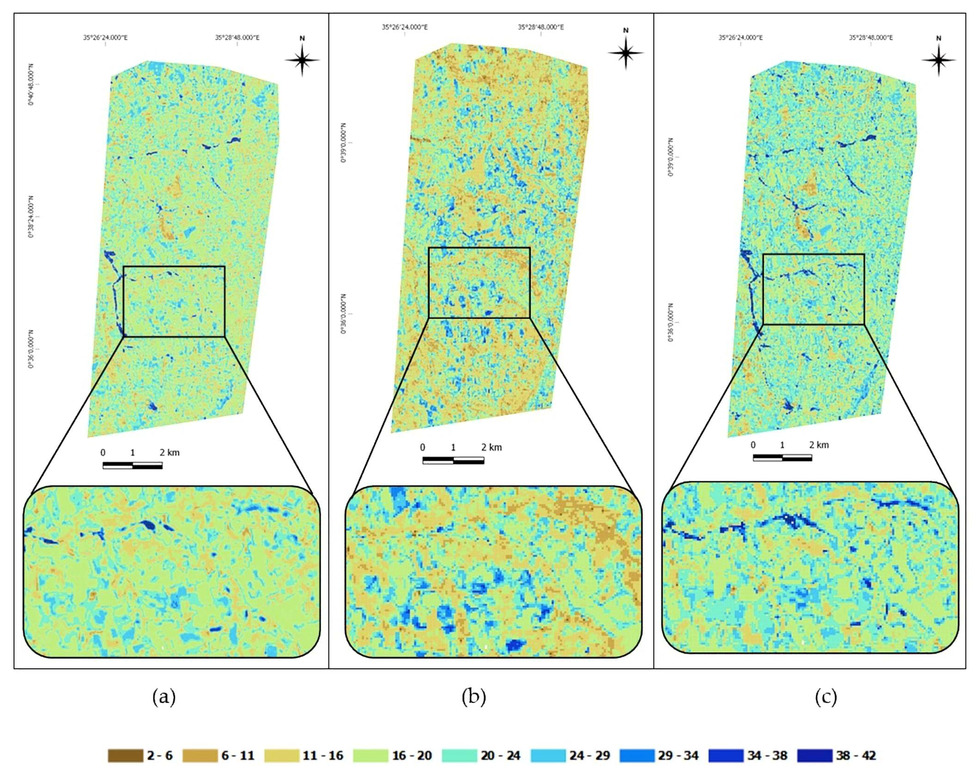
4. Results and Discussion

As illustrated in the flowchart presented in Figure 2, after preparing the radar and optical data and extracting the most relevant features using the RF-RFE method, SVR training was performed as the machine learning algorithm used in this research. Many studies have highlighted the importance of exploiting additional vegetation information provided by optical remote sensing for retrieving soil moisture from a vegetated area [21,22,23,45,46,47]. The indices NDVI and LAI are among the most widely used vegetation indices. With this in mind, we tried to broaden the range of vegetation indices in this study (Table 2). Our study confirms previous findings in the literature regarding the significance of using vegetation indices in a soil moisture retrieval process in vegetated areas. However, in this context, we found that other indices, such as GNDVI, GEMI, DVI, and FCOVER, have the potential to attract more attention. Future studies in other regions and for other data are required to validate this issue. In this study, we also adopted GLCM texture features extracted from radar data. Few researchers have addressed the use of texture features in the domain of soil moisture estimation from SAR data. Our experiments demonstrate that adopting texture features was less important than other features (Figure 3). However, in this study, the GLCM-MEAN feature has been included as one of the selected features in both the pixel-based and object-based approaches (Figure 5). It seems that this feature has been able to increase the retrieval accuracy in combination with other features.

Considering the numerous configurations available to conduct segmentation, it was necessary to choose the best configuration for each scene. It can be seen in Table 3 that the optimal values for the shape and compactness parameters have less variation than the scale parameter for the studied areas. The variation intervals are [0–0.2], [0.4–0.6], and [2–15] for the shape, compactness, and scale parameters, respectively. Object size and consequently the scale parameter appears to have wider variations than those of the shape parameters in the five study areas. However, this difference is minimal for the same region (Uasin Gishu) at two different dates (the scale parameter equals to 11 and 12 for Uasin Gishu on 3 October 2016 and 18 April 2016, respectively). This issue seems to be logical due to the fact that areas with similar characteristics, in terms of input layers to the segmentation process, are expected to have similar segmentation outputs. It seems reasonable to assign values of 0.1 and 0.5 to the shape and compactness parameters and focus more on finding the optimal scale parameter in future studies.

After the training stage and by using the generated model, the soil moisture retrieval was executed for all of the pixels in the image. The advantage of soil moisture retrieval at the pixel level is that there is no need to perform segmentation and to find the appropriate settings in order to obtain optimal image objects. Therefore, this method has less complexity in terms of implementation. As exhibited in Figure 6 and inferred from the accuracy assessment measures, this method has high accuracy in soil moisture retrieval. Nevertheless, in the display of soil moisture at the pixel level, there is a kind of Salt-and-pepper noise. The first column of Figure 7 displays the soil moisture map obtained from the pixel-based approach for the Uasin Gishu scene. The most dominant land use and land cover (LULC) classes available in this scene are cropland, grassland, riverine, and wetland. The riverine and wetland areas can be seen as dark blue pixels in the produced soil moisture map. The SMC maps for all scenes are omitted to conserve space.

In order to obtain optimal soil moisture retrieval at the plot scale, the image objects have to appropriately represent the reality in the field in relation to the soil moisture variable. For this purpose, in this paper, the six features which were selected for the pixel-based approach were used as an input for the multiresolution segmentation algorithm. The use of these six features is expected to result in the most robust image objects in relation to the soil moisture. The weight of each of the six layers in the segmentation process was considered to be equal to 1.

It should be noted that we considered different criteria for weighting the selected features. The importance of each feature or corresponding coefficients of each feature extracted from multiple regression were the two criteria which were considered. However, there was no significant difference in the final results. After segmentation and production of the image objects, the best features in the object space were selected.

Figure 5 depicts the selected features for object-based approach. Having executed the SVR training and model extraction, the soil moisture retrieval was performed for all the image objects. Figure 6 shows the retrieval accuracy in this method. As is observed, the accuracy of the object-based method experienced a diminishment in comparison with the pixel-based one. This was already reported in Figure 5. In order to examine the reason for the decrease, it should be noted that in the object-based approach, each field sample represents a specific amount of soil moisture in an image object (a group of pixels); however, the in situ field measurement is in the form of points where each field sample represents the soil moisture for a pixel. Because there is a possibility of assigning more than one field sample to an image object, the whole process of soil moisture retrieval in the object-based approach is influenced, including the segmentation, feature selection, and the training stage. Therefore, if several soil moisture field measurements belong to an image object in the process of segmentation and production of image objects, the average of the measured field soil moisture values will be attributed to that image object. Moreover, finding the optimal configuration of the segmentation will be based on the same values of the mean soil moisture values. Subsequently, this will be also influential at the feature selection stage. Bearing this in mind, the number of samples used in the SVR training phase in the object-based mode had a reduction from 164 to 110 samples in comparison with the pixel-based category. It is expected that such a reduction in the number of the samples used to carry out the training will affect the quality of the training phase in this approach. Hence, it seems that the field samples could better represent the existing fields in the object-based mode and could increase the accuracy and robustness of the object-based approach if the field sampling phase was initially undertaken at the plot scale. It is worth noting that in this research, a weighted averaging technique was used to allocate more weights to those field samples which had closer corresponding values in the pixel space. This is in comparison with the mean values of the selected feature in the object space. The final accuracy was not affected to a significant degree using this approach. The second column in Figure 7 indicates the soil moisture map compiled by this approach. As is evident from the figure, in the retrieval through the object-based mode, an underestimation has occurred so that the range of the retrieved soil moisture values in the pixel-based mode covers values in the range of 1 to 48%, whereas in the object-based mode this range is 1 to 37%. This stems from the averaging nature of this approach and its effect on the training phase. A more detailed look at the measured and estimated values (Figure 6) revealed overestimation and underestimation in soil moisture estimation for dry and wet zones, respectively. Although this is the case for both approaches, the magnitude of over and underestimation is higher in the object-based approach. The probable reason for this is that the variability of the features is too low to reflect the variability of the target. This issue is clear for riverine and wetland areas in the produced SMC map using the object-based approach (the second column of Figure 7). This SMC map proves that the underestimation rate for these wet areas is higher than that for the produced map using the pixel-based approach. Meanwhile, the object-based approach has shown a more homogeneous behavior and over and underestimation happened almost for all samples belonging to dry and wet zones. However, in the pixel-based approach, for some samples, the opposite behavior has happened. This behavior also stems from the averaging nature of the object-based approach that originates from the segmentation process. This indicates the importance of this stage for making robust image objects and subsequently robust estimation in a soil moisture retrieval process using an OBIA approach.

To resolve this issue, both the pixel-based and the object-based approaches could be integrated. To fulfil this, the output model derived from the pixel-based approach is used to retrieve the soil moisture at the plot scale. In this case, it is expected to eliminate the problems caused by calculations at the object level—allocating the measured point soil moisture to a group of pixels and the necessity of averaging the field samples belonging to an image object—while retrieving the soil moisture at the object level. In other words, the steps related to feature selection and learning are taken at the pixel level and the soil moisture retrieval step is done at the object level. In this case, the scale parameter is used to perform the segmentation and production of image objects and the soil moisture retrieval based on the user’s demand and is independent of the feature selection and learning steps. Practically, this would lead to a determination on the plot scale and the summarization level from the user’s side.

The third column in Figure 7 exhibits the output of this method. It is worth noting that, as expected, the output SMC map of the combined method is much more similar to pixel-based method (zoomed area in Figure 7). This result seem to be realistic given the fact that we used the extracted model from the pixel-based method to estimate the soil moisture for the generated image objects. In this study, the values of 1, 0.1, and 0.5 were used for the scale, shape, and compactness parameters, respectively. This configuration resulted in the production of the soil moisture map in an appropriate plot scale. In this study, in order to have image objects as close as possible to the size of the pixel in the pixel-based method, and to better compare the outputs of both the pixel- and object-based methods, the value of 1 is assigned to the scale parameter. However, according to user requirements, it is possible to increase the scale parameter and produce larger image objects (smaller plot scale) and calculate soil moisture content in a wider area. It is also possible to assign more weight to the shape parameter if this potential exists (for example, in areas with agricultural lands). The minimum and maximum areas of the image objects (in pixels) generated using this configuration for the Kajiado, Machakos, Narok, Uasin Gishu 3 October 2016, and Uasin Gishu 18 April 2016 scenes are equal to [1, 4], [1, 6], [1, 4], [1, 5], and [1, 4], respectively. It should be noted that the resampled pixel size of the used images and the scale of the plot considered by the user will have a direct impact on the configuration. In this study, the process of finding the appropriate configuration was made by visual examination. The authors of this paper intend to investigate the possibility of developing a semi-automatic method in order to find the optimal configuration to produce image objects in accordance with the external reality (in terms of size and shape) in their future studies.

5. Conclusions

This paper has investigated the possibility of soil moisture retrieval at the plot scale using object-based image analysis (OBIA) in vegetated areas. A range of extracted features from Sentinel-1 VV polarization (backscattering coefficient, texture features) and Sentinel-2 (soil, water, and vegetation indices) data were used to assess the capacity of the presented approach. The random forest-recursive feature elimination method was adopted to select the most relevant features for a soil moisture variable. The selected features were processed by means of an advanced regression algorithm based on a SVR approach to retrieve soil moisture content. We have presented a novel approach to retrieve soil moisture at the plot scale. In this approach, we work on image objects instead of pixels. This could conceivably lead to soil moisture estimation at the plot scale with a better representation of the reality of the land cover in vegetated areas. This approach will also result in reduced noise and increased readability of the results. The most important limitation of this approach is that the field measurement phase was initially undertaken at the point scale. This limitation no longer applies by using the combined pixel and object-based approach. The proposed methodology can provide an SMC map with acceptable accuracy (4.94-vol. % RMSE) at the plot scale. On account of the fact that the data used in this study did not represent the best possible scenario (single polarization (VV)-C band radar data in areas with dominant vegetation cover), this work has revealed that the proposed approach meets the requirements to be applied in operational missions. As noted earlier, the scenario used in this research is considered a challenging scenario. This comes from the characteristics of the used data for the study area. In this research, C-band Sentinel-1 data in VV polarization have been used to study the areas with dominant vegetation cover. With this in mind, the resulting accuracy is acceptable. It seems that the use of polarimetric data or data in the L band will result in improved accuracy. To further our research, we intend to examine the proposed algorithm on data and case studies with different characteristics.

References

1. Kornelsen, K.C.; Coulibaly, P. Advances in soil moisture retrieval from synthetic aperture radar and hydrological applications. J. Hydrol. 2013, 476, 460–489. [Google Scholar] [CrossRef]
2. Wang, J.R. The dielectric properties of soil-water mixtures at microwave frequencies. Radio Sci. 1980, 15, 977–985. [Google Scholar] [CrossRef] [Green Version]
3. Kerr, Y.H.; Waldteufel, P.; Wigneron, J.-P.; Delwart, S.; Cabot, F.; Boutin, J.; Escorihuela, M.-J.; Font, J.; Reul, N.; Gruhier, C.; et al. The SMOS Mission: New Tool for Monitoring Key Elements ofthe Global Water Cycle. Proc. IEEE 2010, 98, 666–687. [Google Scholar] [CrossRef] [Green Version]
4. Mecklenburg, S.; Drusch, M.; Kerr, Y.H.; Font, J.; Martin-Neira, M.; Delwart, S.; Buenadicha, G.; Reul, N.; Daganzo-Eusebio, E.; Oliva, R.; et al. ESA’s Soil Moisture and Ocean Salinity Mission: Mission Performance and Operations. IEEE Trans. Geosci. Remote Sens. 2012, 50, 1354–1366. [Google Scholar] [CrossRef] [Green Version]
5. Kerr, Y.H.; Waldteufel, P.; Wigneron, J.-P.; Martinuzzi, J.; Font, J.; Berger, M. Soil moisture retrieval from space: The Soil Moisture and Ocean Salinity (SMOS) mission. IEEE Trans. Geosci. Remote Sens. 2001, 39, 1729–1735. [Google Scholar] [CrossRef]
6. Entekhabi, D.; Njoku, E.G.; O’Neill, P.E.; Kellogg, K.H.; Crow, W.T.; Edelstein, W.N.; Entin, J.K.; Goodman, S.D.; Jackson, T.J.; Johnson, J.; et al. The Soil Moisture Active Passive (SMAP) Mission. Proc. IEEE 2010, 98, 704–716. [Google Scholar] [CrossRef]
7. Entekhabi, D.; Yueh, S.; O’Neill, P.; Kellogg, K.; Allen, A.; Bindlish, R.; Brown, M.; Chan, S.; Colliander, A.; Crow, T.W.; et al. SMAP Handbook; JPL Publication JPL 400-1567; Jet Propulsion Laboratory: Pasadena, CA, USA, 2014; 182p. [Google Scholar]
8. Wagner, W.; Lemoine, G.; Rott, H. A Method for Estimating Soil Moisture from ERS Scatterometer and Soil Data. Remote Sens. Environ. 1999, 70, 191–207. [Google Scholar] [CrossRef]
9. Bartalis, Z.; Wagner, W.; Naeimi, V.; Hasenauer, S.; Scipal, K.; Bonekamp, H.; Figa, J.; Anderson, C. Initial soil moisture retrievals from the METOP-A Advanced Scatterometer (ASCAT). Geophys. Res. Lett. 2007, 34, L20401. [Google Scholar] [CrossRef]
10. Zhang, X.; Zhao, J.; Sun, Q.; Wang, X.; Guo, Y.; Li, J. Soil Moisture Retrieval from AMSR-E Data in Xinjiang (China): Models and Validation. IEEE J. Sel. Top. Appl. Earth Obs. Remote Sens. 2011, 4, 117–127. [Google Scholar] [CrossRef]
11. Baghdadi, N.; Cerdan, O.; Zribi, M.; Auzet, V.; Darboux, F.; el Hajj, M.; Kheir, R.B. Operational performance of current synthetic aperture radar sensors in mapping soil surface characteristics in agricultural environments: Application to hydrological and erosion modelling. Hydrol. Process. 2008, 22, 9–20. [Google Scholar] [CrossRef]
12. Le Hegarat-Mascle, S.; Zribi, M.; Alem, F.; Weisse, A.; Loumagne, C. Soil moisture estimation from ERS/SAR data: Toward an operational methodology. IEEE Trans. Geosci. Remote Sens. 2002, 40, 2647–2658. [Google Scholar] [CrossRef]
13. Balenzano, A.; Mattia, F.; Satalino, G.; Davidson, M.W.J. Dense Temporal Series of C- and L-band SAR Data for Soil Moisture Retrieval Over Agricultural Crops. IEEE J. Sel. Top. Appl. Earth Obs. Remote Sens. 2011, 4, 439–450. [Google Scholar] [CrossRef]
14. Merzouki, A.; McNairn, H.; Pacheco, A. Mapping Soil Moisture Using RADARSAT-2 Data and Local Autocorrelation Statistics. IEEE J. Sel. Top. Appl. Earth Obs. Remote Sens. 2011, 4, 128–137. [Google Scholar] [CrossRef]
15. Zribi, M.; Dechambre, M. A new empirical model to retrieve soil moisture and roughness from C-band radar data. Remote Sens. Environ. 2003, 84, 42–52. [Google Scholar] [CrossRef]
16. Fung, A.K.; Liu, W.Y.; Chen, K.S.; Tsay, M.K. An Improved Iem Model for Bistatic Scattering from Rough Surfaces. J. Electromagn. Waves Appl. 2002, 16, 689–702. [Google Scholar] [CrossRef]
17. Attema, E.P.W.; Ulaby, F.T. Vegetation modeled as a water cloud. Radio Sci. 1978, 13, 357–364. [Google Scholar] [CrossRef]
18. Oh, Y.; Sarabandi, K.; Ulaby, F.T. Semi-empirical model of the ensemble-averaged differential Mueller matrix for microwave backscattering from bare soil surfaces. IEEE Trans. Geosci. Remote Sens. 2002, 40, 1348–1355. [Google Scholar] [CrossRef] [Green Version]
19. Oh, Y. Quantitative Retrieval of Soil Moisture Content and Surface Roughness from Multipolarized Radar Observations of Bare Soil Surfaces. IEEE Trans. Geosci. Remote Sens. 2004, 42, 596–601. [Google Scholar] [CrossRef]
20. Dubois, P.C.; vanZyl, J.; Engman, T. Corrections to ‘Measuring Soil Moisture with Imaging Radars’. IEEE Trans. Geosci. Remote Sens. 1995, 33, 915–926. [Google Scholar] [CrossRef]
21. Fung, A.K.; Li, Z.; Chen, K.S. Backscattering from a Randomly Rough Dielectric Surface. IEEE Trans. Geosci. Remote Sens. 1992, 30, 356–369. [Google Scholar] [CrossRef]
22. Zribi, M.; Taconet, O.; le Hégarat-Mascle, S.; Vidal-Madjar, D.; Emblanch, C.; Loumagne, C.; Normand, M. Backscattering behavior and simulation comparison over bare soils using SIR-C/X-SAR and ERASME 1994 data over Orgeval. Remote Sens. Environ. 1997, 59, 256–266. [Google Scholar] [CrossRef]
23. Baghdadi, N.; Holah, N.; Zribi, M. Calibration of the Integral Equation Model for SAR data in C-band and HH and VV polarizations. Int. J. Remote Sens. 2006, 27, 805–816. [Google Scholar] [CrossRef]
24. Baghdadi, N.; Zribi, M. Evaluation of radar backscatter models IEM, OH and Dubois using experimental observations. Int. J. Remote Sens. 2006, 27, 3831–3852. [Google Scholar] [CrossRef]
25. Sahebi, M.R.; Bonn, F.; Gwyn, Q.H.J. Estimation of the moisture content of bare soil from RADARSAT-1 SAR using simple empirical models. Int. J. Remote Sens. 2003, 24, 2575–2582. [Google Scholar] [CrossRef]
26. Oh, Y.; Sarabandi, K.; Ulaby, F.T. An empirical model and an inversion technique for radar scattering from bare soil surfaces. IEEE Trans. Geosci. Remote Sens. 1992, 30, 370–381. [Google Scholar] [CrossRef]
27. Mattia, F.; Satalino, G.; Pauwels, V.R.N.; Loew, A. Soil moisture retrieval through a merging of multi-temporal L-band SAR data and hydrologic modelling. Hydrol. Earth Syst. Sci. Discuss. 2008, 5, 3479–3515. [Google Scholar] [CrossRef]
28. Prakash, R.; Singh, D.; Pathak, N.P. A fusion approach to retrieve soil moisture with SAR and optical data. IEEE J. Sel. Top. Appl. Earth Obs. Remote Sens. 2012, 5, 196–206. [Google Scholar] [CrossRef]
29. Baghdadi, N.; el Hajj, M.; Zribi, M.; Fayad, I. Coupling SAR C-Band and Optical Data for Soil Moisture and Leaf Area Index Retrieval over Irrigated Grasslands. IEEE J. Sel. Top. Appl. Earth Obs. Remote Sens. 2016, 9, 1229–1243. [Google Scholar] [CrossRef]
30. Gao, Q.; Zribi, M.; Escorihuela, M.J.; Baghdadi, N. Synergetic use of sentinel-1 and sentinel-2 data for soil moisture mapping at 100 m resolution. Sensors 2017, 17, 1966. [Google Scholar] [CrossRef] [PubMed]
31. El Hajj, M.; Baghdadi, N.; Zribi, M.; Bazzi, H. Synergic use of Sentinel-1 and Sentinel-2 images for operational soil moisture mapping at high spatial resolution over agricultural areas. Remote Sens. 2017, 9, 1292. [Google Scholar] [CrossRef]
32. Kolassa, J.; Reichle, R.H.; Draper, C.S. Merging active and passive microwave observations in soil moisture data assimilation. Remote Sens. Environ. 2017, 191, 117–130. [Google Scholar] [CrossRef]
33. Kolassa, J.; Gentine, P.; Prigent, C.; Aires, F.; Alemohammad, S.H. Soil moisture retrieval from AMSR-E and ASCAT microwave observation synergy. Part 2: Product evaluation. Remote Sens. Environ. 2017, 195, 202–217. [Google Scholar] [CrossRef]
34. Panciera, R.; Walker, J.P.; Kalma, J.D.; Kim, E.J.; Hacker, J.M.; Merlin, O.; Berger, M.; Skou, N. The NAFE’05/CoSMOS Data Set: Toward SMOS Soil Moisture Retrieval, Downscaling, and Assimilation. IEEE Trans. Geosci. Remote Sens. 2008, 46, 736–745. [Google Scholar] [CrossRef] [Green Version]
35. Merlin, O.; Walker, J.P.; Chehbouni, A.; Kerr, Y. Towards deterministic downscaling of SMOS soil moisture using MODIS derived soil evaporative efficiency. Remote Sens. Environ. 2008, 112, 3935–3946. [Google Scholar] [CrossRef] [Green Version]
36. Piles, M.; Camps, A.; Vall-llossera, M.; Corbella, I.; Panciera, R.; Rudiger, C.; Kerr, Y.H.; Walker, J. Downscaling SMOS-Derived Soil Moisture Using MODIS Visible/Infrared Data. IEEE Trans. Geosci. Remote Sens. 2011, 49, 3156–3166. [Google Scholar] [CrossRef]
37. Peng, J.; Loew, A.; Zhang, S.; Wang, J.; Niesel, J. Spatial Downscaling of Satellite Soil Moisture Data Using a Vegetation Temperature Condition Index. IEEE Trans. Geosci. Remote Sens. 2016, 54, 558–566. [Google Scholar] [CrossRef]
38. NASA Focused on Sentinel as Replacement for SMAP Radar. Available online: http://spacenews.com/nasa-focused-on-sentinel-as-replacement-for-smap-radar/ (accessed on 2 January 2018).
39. Colliander, A.; Fisher, J.B.; Halverson, G.; Merlin, O.; Misra, S.; Bindlish, R.; Jackson, T.J.; Yueh, S. Spatial Downscaling of SMAP Soil Moisture Using MODIS Land Surface Temperature and NDVI During SMAPVEX15. IEEE Geosci. Remote Sens. Lett. 2017, 14, 2107–2111. [Google Scholar] [CrossRef]
40. Chakrabarti, S.; Bongiovanni, T.; Judge, J.; Nagarajan, K.; Principe, J.C. Downscaling Satellite-Based Soil Moisture in Heterogeneous Regions Using High-Resolution Remote Sensing Products and Information Theory: A Synthetic Study. IEEE Trans. Geosci. Remote Sens. 2015, 53, 85–101. [Google Scholar] [CrossRef]
41. Clewley, D.; Whitcomb, J.B.; Akbar, R.; Silva, A.R.; Berg, A.; Adams, J.R.; Caldwell, T.; Entekhabi, D.; Moghaddam, M. A Method for Upscaling In Situ Soil Moisture Measurements to Satellite Footprint Scale Using Random Forests. IEEE J. Sel. Top. Appl. Earth Obs. Remote Sens. 2017, 10, 2663–2673. [Google Scholar] [CrossRef]
42. Gherboudj, I.; Magagi, R.; Berg, A.A.; Toth, B. Characterization of the Spatial Variability of In-Situ Soil Moisture Measurements for Upscaling at the Spatial Resolution of RADARSAT-2. IEEE J. Sel. Top. Appl. Earth Obs. Remote Sens. 2017, 10, 1813–1823. [Google Scholar] [CrossRef]
43. Aubert, M.M.; Baghdadi, N.; Zribi, M.; Ose, K.; el Hajj, M.; Vaudour, E. Gonzalez-sosa Toward an Operational Bare Soil Moisture Mapping Using TerraSAR-X Data Acquired Over Agricultural Areas. IEEE J. Sel. Top. Appl. Earth Obs. Remote Sens. 2013, 6, 900–916. [Google Scholar] [CrossRef] [Green Version]
44. Paloscia, S.; Pettinato, S.; Santi, E.; Notarnicola, C.; Pasolli, L.; Reppucci, A. Soil moisture mapping using Sentinel-1 images: Algorithm and preliminary validation. Remote Sens. Environ. 2013, 134, 234–248. [Google Scholar] [CrossRef]
45. Pasolli, L.; Notarnicola, C.; Bertoldi, G.; Bruzzone, L.; Remelgado, R.; Greifeneder, F.; Niedrist, G.; della Chiesa, S.; Tappeiner, U.; Zebisch, M. Estimation of soil moisture in mountain areas using SVR technique applied to multiscale active radar images at C-band. IEEE J. Sel. Top. Appl. Earth Obs. Remote Sens. 2015, 8, 262–283. [Google Scholar] [CrossRef]
46. Tiffen, M.; Mortimore, M. Environment, Population Growth and Productivity in Kenya: A Case Study of Machakos District. Dev. Policy Rev. 1992, 10, 359–387. [Google Scholar] [CrossRef]
47. Kenya. Sustainable Development Knowledge Platform. Available online: https://sustainabledevelopment.un.org/memberstates/kenya (accessed on 25 June 2018).
48. El Hajj, M.; Baghdadi, N.; Zribi, M.; Angelliaume, S. Analysis of Sentinel-1 Radiometric Stability and Quality for Land Surface Applications. Remote Sens. 2016, 8, 406. [Google Scholar] [CrossRef] [Green Version]
49. Louis, J.; Debaecker, V.; Pflug, B.; Main-Knorn, M.; Bieniarz, J.; Mueller-Wilm, U.; Cadau, E.; Gascon, F. Sentinel-2 SEN2COR: L2A Processor for Users; (Special Publication) ESA SP-740; European Space Agency: Prague, Czech Repubic, 2016. [Google Scholar]
50. Haralick, R.M.; Shanmugam, K.; Dinstein, I. Textural Features for Image Classification. IEEE Trans. Syst. Man. Cybern. 1973, SMC-3, 610–621. [Google Scholar] [CrossRef]
51. Anys, H.; He, D.-C. Evaluation of textural and multipolarization radar features for crop classification. IEEE Trans. Geosci. Remote Sens. 1995, 33, 1170–1181. [Google Scholar] [CrossRef]
52. Soh, L.-K.; Tsatsoulis, C. Texture analysis of SAR sea ice imagery using gray level co-occurrence matrices. IEEE Trans. Geosci. Remote Sens. 1999, 37, 780–795. [Google Scholar] [CrossRef] [Green Version]
53. Cui, M.; Prasad, S.; Mahrooghy, M.; Aanstoos, J.V.; Lee, M.A.; Bruce, L.M. Decision Fusion of Textural Features Derived From Polarimetric Data for Levee Assessment. IEEE J. Sel. Top. Appl. Earth Obs. Remote Sens. 2012, 5, 970–976. [Google Scholar] [CrossRef]
54. STEP. Documentation. Available online: http://step.esa.int/main/doc/ (accessed on 24 February 2018).
55. Arbib, M.A. The Handbook of Brain Theory and Neural Networks; MIT Press: Cambridge, MA, USA, 1998. [Google Scholar]
56. Guyon, I.; Weston, J.; Barnhill, S.; Vapnik, V. Gene Selection for Cancer Classification using Support Vector Machines. Mach. Learn. 2002, 46, 389–422. [Google Scholar] [CrossRef] [Green Version]
57. Zhang, R.; Ma, J. Feature selection for hyperspectral data based on recursive support vector machines. Int. J. Remote Sens. 2009, 30, 3669–3677. [Google Scholar] [CrossRef]
58. Baatz, M.; Benz, U.; Dehghani, S.; Heynen, M.; Holtje, A.; Hofmann, P.; Lingenfelder, I.; Mimler, M.; Sohlbach, M.; Weber, M.; et al. eCognition Professional: User Guide 4; Definiens Imaging GmbH: München, Germeny, 2004. [Google Scholar]
59. Benz, U.C.; Hofmann, P.; Willhauck, G.; Lingenfelder, I.; Heynen, M. Multi-resolution, object-oriented fuzzy analysis of remote sensing data for GIS-ready information. ISPRS J. Photogramm. Remote Sens. 2004, 58, 239–258. [Google Scholar] [CrossRef] [Green Version]
60. Nussbaum, S.; Menz, G. Object-Based Image Analysis and Treaty Verification: New Approaches in Remote Sensing—Applied to Nuclear Facilities in Iran; Springer: Berlin, Germany, 2008. [Google Scholar]
61. Pasolli, L.; Notarnicola, C.; Bruzzone, L. Estimating soil moisture with the support vector regression technique. IEEE Geosci. Remote Sens. Lett. 2011, 8, 1080–1084. [Google Scholar] [CrossRef]
62. Bruzzone, L.; Melgani, F. Robust multiple estimator systems for the analysis of biophysical parameters from remotely sensed data. IEEE Trans. Geosci. Remote Sens. 2005, 43, 159–174. [Google Scholar] [CrossRef]
63. Vapnik, V.N. The Nature of Statistical Learning Theory; Springer: Berlin, Germany, 2000. [Google Scholar]
Figure 1. Location of study sites in Kenya: Uasin Gishu, Narok, Kajiado, and Machakos; Typical land use and land cover (LULC) classes in the study site: (a) cropland; (b) shrubland; (c) grassland; and (d) bare land; (e) in situ measurements location.
Remotesensing 10 01285 g001
Figure 2. Proposed flowchart for soil moisture retrieval using the pixel- and object-based approach. SVR, support vector regression; SMC, soil moisture content.
Remotesensing 10 01285 g002
Figure 3. Importance of all extracted features.
Remotesensing 10 01285 g003
Figure 4. Demonstration of the R Square for each segmentation configuration (scale, shape, and compactness parameters) for the Machakos scene.
Remotesensing 10 01285 g004
Figure 5. Different feature subset sizes with the corresponding root mean square error (RMSE) and final selected features for both approaches. PB, pixel-based; OB, object-based.
Remotesensing 10 01285 g005
Figure 6. Scatterplot of estimated versus measured SMC (m3/m3) values evaluated on test samples. (left) pixel-based approach; (right) object-based approach.
Remotesensing 10 01285 g006
Figure 7. Final SMC map for the Uasin Gishu 18 April 2016 scene: (a): pixel-based; (b): object-based; (c): combined approach.
Remotesensing 10 01285 g007