Article

Canopy Hyperspectral Sensing of Paddy Fields at the Booting Stage and PLS Regression can Assess Grain Yield

by
Kensuke Kawamura
1,*,
Hiroshi Ikeura
1,
Sengthong Phongchanmaixay
2 and
Phanthasin Khanthavong
2
1
Japan International Research Center for Agricultural Sciences (JIRCAS), Tsukuba, Ibaraki 305-8686, Japan
2
Rice Research Center, National Agriculture and Forestry Research Institute (NAFRI), P.O. Box 7170 Vientiane, Laos
*
Author to whom correspondence should be addressed.
Remote Sens. 2018, 10(8), 1249; https://doi.org/10.3390/rs10081249
Submission received: 26 June 2018 / Revised: 6 August 2018 / Accepted: 6 August 2018 / Published: 8 August 2018
(This article belongs to the Special Issue Remote Sensing in Support of Transforming Smallholder Agriculture)

Abstract

:
Canopy hyperspectral (HS) sensing is a promising tool for estimating rice (Oryza sativa L.) yield. However, the timing of HS measurements is crucial for assessing grain yield prior to harvest because rice growth stages strongly influence the sensitivity to different wavelengths and the evaluation performance. To clarify the optimum growth stage for HS sensing-based yield assessments, the grain yield of paddy fields during the reproductive phase to the ripening phase was evaluated from field HS data in conjunction with iterative stepwise elimination partial least squares (ISE-PLS) regression. The field experiments involved three different transplanting dates (12 July, 26 July, and 9 August) in 2017 for six cultivars with three replicates (n = 3 × 6 × 3 = 54). Field HS measurements were performed on 2 October 2017, during the panicle initiation, booting, and ripening growth stages. The predictive accuracy of ISE-PLS was compared with that of the standard full-spectrum PLS (FS-PLS) via coefficient of determination (R2) values and root mean squared errors of cross-validation (RMSECV), and the robustness was evaluated by the residual predictive deviation (RPD). Compared with the FS-PLS models, the ISE-PLS models exhibited higher R2 values and lower RMSECV values for all data sets. Overall, the highest R2 values and the lowest RMSECV values were obtained from the ISE-PLS model at the booting stage (R2 = 0.873, RMSECV = 22.903); the RPD was >2.4. Selected HS wavebands in the ISE-PLS model were identified in the red-edge (710–740 nm) and near-infrared (830 nm) regions. Overall, these results suggest that the booting stage might be the best time for in-season rice grain assessment and that rice yield could be evaluated accurately from the HS sensing data via the ISE-PLS model.

Graphical Abstract

1. Introduction

Laos is among the major rice (Oryza sativa L.) consuming countries in South-East Asia [1]. Even though Laos achieved self-sufficient rice production status in the late 1990s, and the national economy has continuously grown, rice remains the main staple food for people in Laos, and its demand is continuously growing [2]. Thus, in-season assessment of rice grain yield could benefit farmers and rice-processing industries by quantifying produce supply and market prices. Rice yield can be predicted by crop growth simulation models whose inputs are related to a wide range of environmental variables (e.g., air temperature and solar radiation) [3], and rice yield is generally related to crop growth and the nitrogen (N) status before the heading stage [4,5]. Therefore, indicators related to growth and the N status before the heading stage have been applied in various models to predict yield variation among cultivars [6,7]. However, in Laos and other developing countries, these data may not be readily available because gathering and accumulating such environmental data is difficult.
Canopy hyperspectral (HS) reflectance measurements are increasingly being used as a reliable method for the timely assessment of crop growth and nutritive status [8,9,10]. The timing of the measurements is crucial for the in-season assessment of grain yield because growth stages strongly influence the sensitivity to different wavelengths and the prediction performance [11,12,13]. The spectral signature responds to changes in aboveground biomass (BM), more precisely, leaf area index (LAI) and chlorophyll contents [14]. The green LAI, defined as the one-sided green leaf area per unit horizontal ground area [15], is directly related to the growth status of crops [16] and largely influences the canopy spectral reflectance. Leaf chlorophyll contents are vital pigments for photosynthesis, and can provide information on the physiological state of the crops. The leaf chlorophyll contents are strongly correlated with nitrogen (N) content [17], and can be used for indirect estimation of crop N status at canopy level [18,19]. Moreover, when multiplying LAI by chlorophyll contents (LAI × Chl), it is expected to have a more robust relationship with canopy N status among years and development stages [18].
A common and widely used approach involves developing relationships between ground-measured biophysical parameters (e.g., LAI and BM) and vegetation indices (VIs) [20,21,22], such as the normalized difference vegetation index (NDVI) [23] and relative vegetation index (RVI) [24]. These VIs perform well during the early stages of crop growth, but the predictive accuracy greatly decreases during the late growth stages, especially after the heading stage. A major issue with the use of VIs centers on canopy reflectance being strongly affected by both structural (e.g., LAI) and biochemical (e.g., chlorophyll) properties of the canopy [25]. During the late period of crop growth, panicles change the canopy structure of crops and affect crop canopy spectral reflectance. The VIs are influenced by saturation effects under moderate to high biomass conditions (LAI > 2.5–3.0 in NDVI) [26]. When the canopy reaches 100% coverage, the amount of red light absorbance by the leaves rapidly reaches a peak, while the near-infrared (NIR) scattering continues to increase. As a result, once the rice canopy is closed, the NIR reflectance will continue to rise, but the red reflectance will show only modest decreases, resulting in only slight changes in the VIs [26].
Most VIs use two or three wavebands, while multivariate analysis can provide more flexibility in choosing individual narrow wavebands and improve the model’s ability to estimate the biophysical or biochemical properties of rice plants [27,28]. Thus, stepwise multiple linear regression (MLR) analysis has been widely used to select critical wavebands for estimating biophysical (biomass, LAI) [12,26,27] and biochemical properties [29,30]. For the MLR analyses, 4–6 wavebands are generally used in the final model to avoid the over-fitting issue. For example, Gnyp et al. [27] developed MLR models to estimate biomass in rice at different growth stages, and obtained the best model at the tillering stage using four wavebands at 672, 696, 814, and 707 nm. Partial least squares (PLS) is another technique that has been widely applied to estimate biophysical and biochemical parameters from field HS measurements [10,31,32]. Unlike MLR, PLS regression is a bilinear calibration method [33] that can treat all available spectral wavebands without multicollinearity issues. PLS was initially used for laboratory spectroscopy but is now increasingly used for analyzing HS data of wheat [34,35,36], maize [37], paddy fields [8,9,32,38] and grasslands [39,40,41,42]. Previous studies have indicated that the selection of appropriate wavebands can refine the predictive ability of the standard full-spectrum PLS (FS-PLS) by optimizing important spectral wavebands [43,44]; therefore, several waveband selection methods have been developed, such as iterative stepwise elimination PLS (ISE-PLS) [45] and genetic algorithm PLS (GA-PLS) [46]. Nonetheless, no study has used the wavelength selection method on PLS to estimate rice yield from canopy reflectance at different growth stages.
In this study, we aimed to clarify the optimal timing for assessing rice yield from field HS measurements in Laos. Using canopy HS data, we also compared the predictive abilities of ISE-PLS and FS-PLS to evaluate the relationship with grain yield during the reproductive stages (panicle initiation and booting) to the ripening stage.

2. Materials and Methods

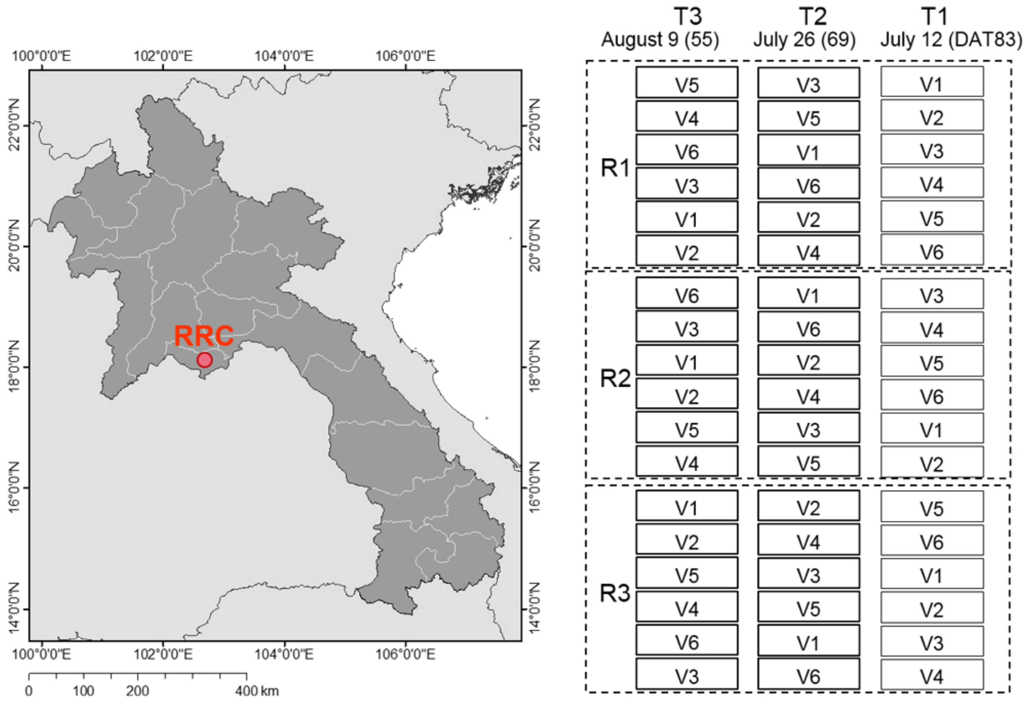
2.1. Experimental Site and Field Design

This study was conducted in an experimental field at the Rice Research Center (RRC) of the National Agriculture and Forestry Research Institute (NAFRI) (18°8′56.65″N, 102°44′9.78″E), in the northern part of Vientiane in Laos (Figure 1). The soil type is characterized by clay loam (CL, 0–30 cm) and light clay (LiC, 40–60 cm).
The experiment was performed during the growing period in 2017 using a randomized complete block design with three replications (R1–R3), shown in Figure 1. Each plot size was 5 m × 2 m. The treatments included three different transplanting dates (T1: 12 July, T2: 26 July, and T3: 8 August) and six rice cultivars (cv.) (V1: cv. Tadokkham [TDK] 8, V2: cv. TDK11, V3: cv. TSN7, V4: cv. Homsavanh [HSV], V5: cv. Khaophorbane [KPB], and V6: cv. Khaokongkane [KKK]); V4, V5, and V6 were planted in a village in southern Laos, V1, V2, and V3 were improved cultivated varieties expected to be introduced to southern rain-fed paddy fields in the future. In southern Laos, there are wide areas of rain-fed paddy fields and it is also an important area to support rice production.
In all the plots, 30-day-old seedlings were transplanted, and the planting density was 25 hills m−2 (0.2 m × 0.2 m). N-P2O5-K2O (30-30-30; kg ha−1) fertilizer was applied at transplanting, and N (15 kg ha1) was applied at 25 and 50 days after transplanting (DAT). The weeds were controlled by hand when necessary. Irrigation water was continuously supplied during the growing period.

2.2. Plant Sampling and Determination of Grain Yield

The harvest dates varied depending on differences in both the transplanting dates and the rice varieties. Figure 2 shows the transplanting, flowering (start of the heading period), and harvest dates. Plants were sampled on the harvest dates: T1 was harvested from 18 October to 27 October (day of year [DOY] = 291–300), T2 was harvested from 27 October–10 November (300–314), and T3 was harvested from 6 November to 16 November (314–320) in 2017. At each sampling, the biomass (BM) was collected by clipping ten rice hills (each hill had 3 rice plants) as five hills from the 4th and 6th columns among the ten rows (every four hills in the middle) of each plot to avoid a border effect [47,48], defined as the difference in the performance between external plants and internal plants in a plot. The rice yield was estimated at a 14% moisture content (MC) for each treatment.

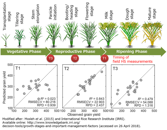
2.3. Canopy HS Measurements

Canopy HS measurements were carried out on 2 October 2017. On that date, the rice growth stages at T1, T2, and T3 included the ripening (with the exception of V4), booting, and panicle initiation stages, respectively. To help explain the timing, Figure 3 shows the days to flowering (DTF) and days to harvest (DTH) from the date of the HS field measurements. The negative values of DTF and DTH indicate the number of days before flowering or harvesting, respectively, while the positive DTF values indicate the number of days after flowering. The mean DTF values of the T1, T2, and T3 data sets were 4.11, −4.83, and −13.9 days, respectively, and the mean DTH values of the T1, T2, and T3 data sets were −20.5, −30.7, and −39.2 days, respectively.
Canopy reflectance spectra were obtained using a portable MS-720 spectroradiometer (EKO Instruments, Tokyo, Japan). The spectroradiometer has a spectral sampling wavelength of 3.3 nm in the 350–1050 nm range, which was reproduced as a 1 nm-resolution wavelength for outputting the data using MS720 software ver. 1.0 (EKO Instruments, Tokyo, Japan). A Spectralon reference panel (Labsphere, Inc., Sutton, NH, USA) was used to optimize the MS720 prior to capturing every five canopy reflectance measurements at each plot. The five spectral readings per plot were averaged for further analyses. The measurements were performed between 12:30 and 14:00 local time (GST+7) on a clear-sky day. For the irrigated rice field, the water and soil background influence the plant canopy reflectance [49,50], especially in the early growth stage when the vegetation cover is low. To reduce the background effects, the sensor head was held approximately 60 cm above the canopy at nadir. The radiometer had a 25° field of view (FOV), producing a view area with a 22 cm diameter at the canopy level.

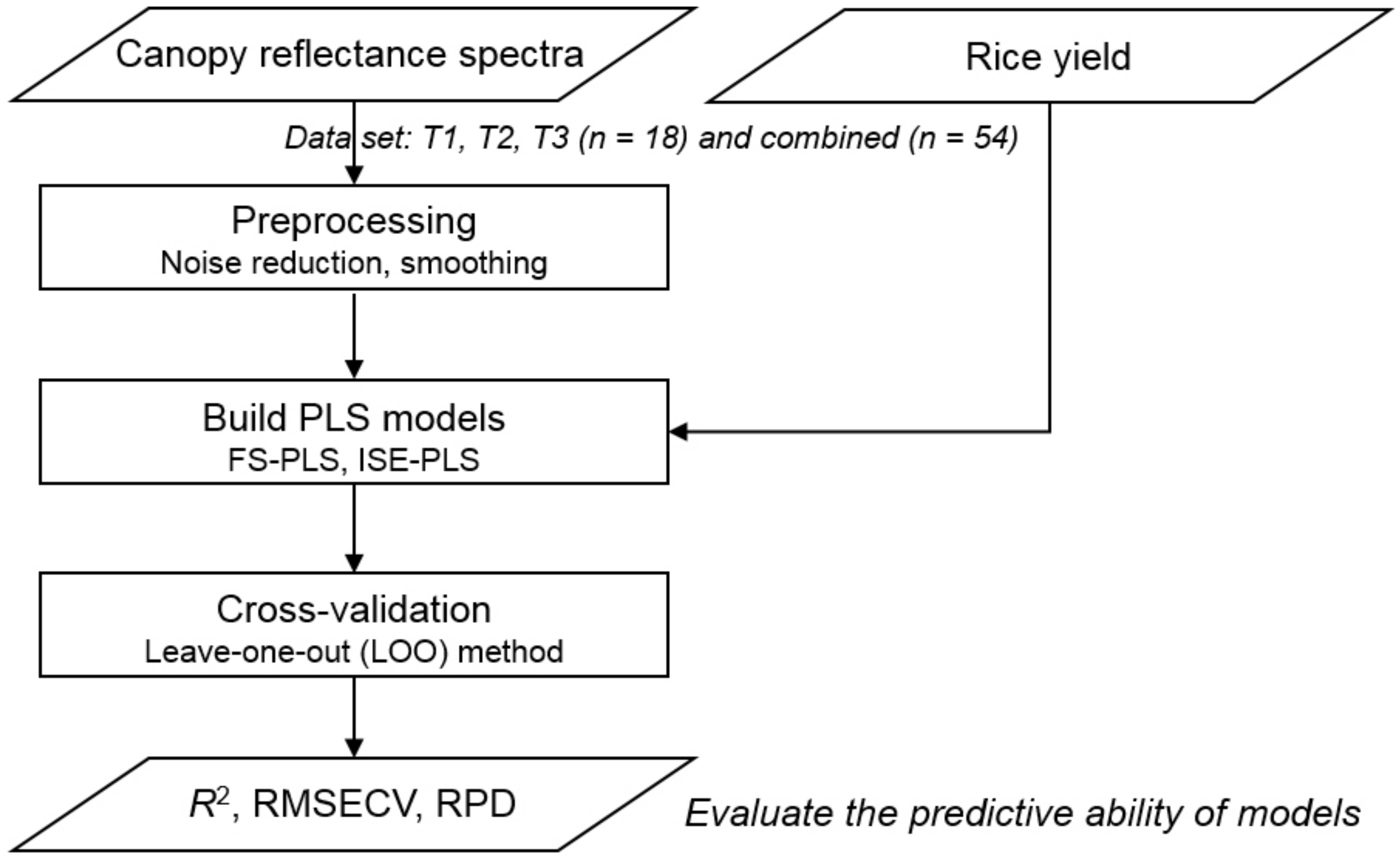
2.4. Preprocessing of Spectral Data

To make the data processing easier to understand, Figure 4 shows a flowchart depicting a general overview of the methodology.
The spectral data in both edge wavelength regions (350–399 nm and 931–1050 nm) were eliminated due to a low signal-to-noise ratio generated by the instrument; the remaining 531 bands (400–930 nm) were used for analyses. The spectral data were smoothed using the Savitsky-Golay smoothing filter [51]. A third-order, 15-band moving polynomial was fitted via the original reflectance signatures.

2.5. PLS Regression Analysis

FS-PLS and ISE-PLS were performed using smoothed reflectance data to evaluate the BM and grain yield for all combined data (n = 54) and for the T1, T2, and T3 data sets (n = 18), respectively. The FS-PLS equation is described as follows:
y   =   β 1 x 1 + β 2 x 2 +     +   β k x k   +   ε
where the response variable y is a vector of the grain yield, the explanatory variables x1 to xk are the surface reflectance values for spectral bands 1 to k (400, 401, …, 930 nm), β1 to βk are the estimated weighted coefficients, and ε is the error vector. To avoid over-fitting the model, the optimal number of latent variables (NLV) was determined by leave-one-out (LOO) cross-validation, which was based on the minimum value of the root mean squared error of cross-validation (RMSECV) [52]. The RMSECV was calculated as follows:
RMSECV   =   i   =   1 n ( y i     y p ) 2 n
where yi and yp are the measured and predicted grain yields for sample i, respectively, and n is the number of samples in the data set.
With respect to ISE-PLS, the ISE method eliminates noisy variables (wavebands) and selects useful predictors. When PLS models include large numbers of redundant variables or outliers, the models’ predictive abilities may perform poorly, while the ISE method can overcome such problems. The model performance depends on the importance of predictors (zi), which is computed as follows:
z i   =   | β k | s k k   =   1 K | β k | s k
where sk is the standard deviation and βk is the regression coefficient; both sk and βk correspond to the predictor variable of waveband k.
The PLS regression model was first developed using all available wavebands (531 bands, 400–930 nm). To create a scope in which useless predictor variables were removed and the predictive ability was improved, each zk predictor was evaluated, and the minimum values were eliminated for being less-informative wavebands. The PLS model was subsequently re-calibrated with the remaining predictors [53]. The model-building procedure was then repeated until the final model was calibrated with the maximum predictive ability. The final model was that with the maximum predictive ability, as defined by the minimum RMSECV value [54].

2.6. Predictive Ability of PLS Regressions

To assess the predictive abilities of the FS-PLS and ISE-PLS models, the coefficient of determination (R2), RMSECV, and residual predictive deviation (RPD) in conjunction with LOO cross-validation were used in this study. High R2 and low RMSECV values indicate the best model for predicting grain yield. The RPD was defined as the ratio of the standard deviation (SD) of the reference data for predicting the RMSECV [55]. For the performance ability of the calibration models, the RPD is suggested to be at least 3 for agricultural applications; RPD values between 2 and 3 indicate a model with a good predictive ability, 1.5 < RPD < 2 indicates an intermediate model needing improvement, and an RPD < 1.5 indicates that the model has a poor predictive ability [56].
All the data handling and linear regression analyses were performed using Matlab software ver. 9.0 (MathWorks, Sherborn, MA, USA).

3. Results and Discussion
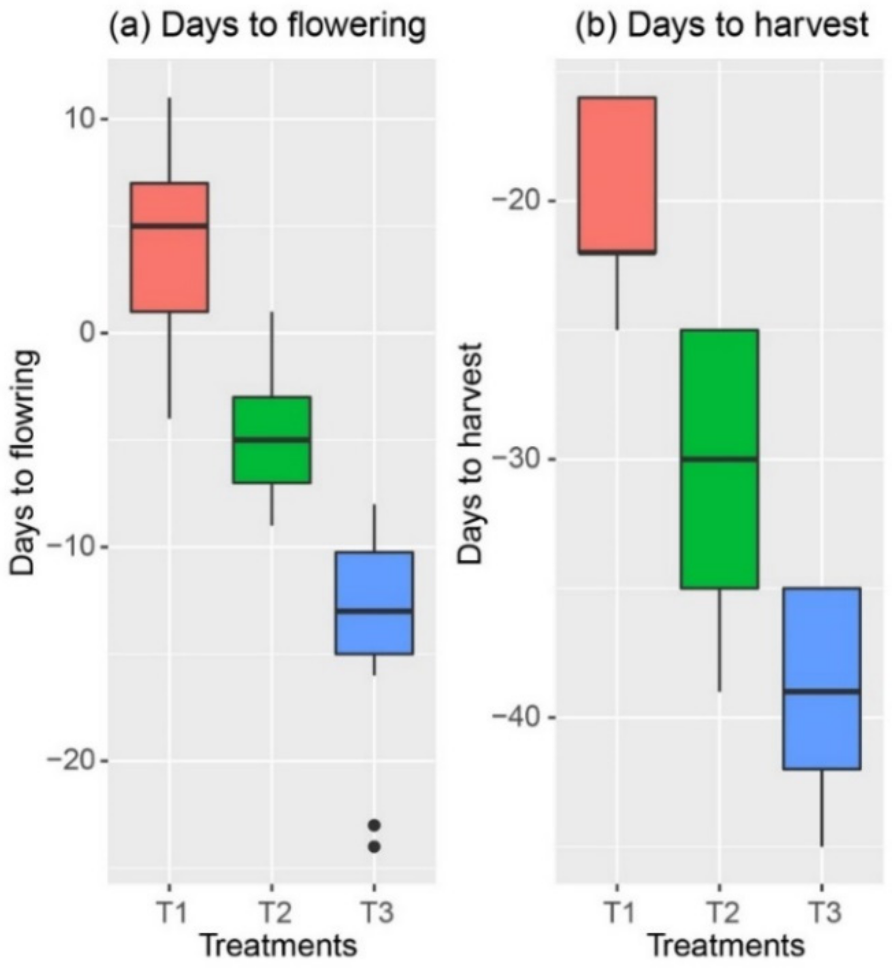
3.1. Grain Yield

The timing of transplanting to paddy fields is an important element to maximize rice productivity under various environments and is closely related to the timing of heading and maturity [57]. Table 1 shows the descriptive analysis results for the grain yield of the combined data set (n = 54) and each individual data set (n = 18). In the combined data set, treatments (transplanting dates and rice varieties) generated a wide range of yield (101.3–462.0 g m−2). Among the data sets, compared with those of T1 (292.9 g m−2, coefficient of variation [CV] = 26.5) and T3 (265.0 g m−2, CV = 27.5), the mean grain yield and variance of T2 were higher (327.9 g m−2) and lower (CV = 17.3), respectively. Although the influence of the variety was included, T2 (26 July) was considered the timing of optimal transplanting to maximize yield (Ikeura et al. unpublished).

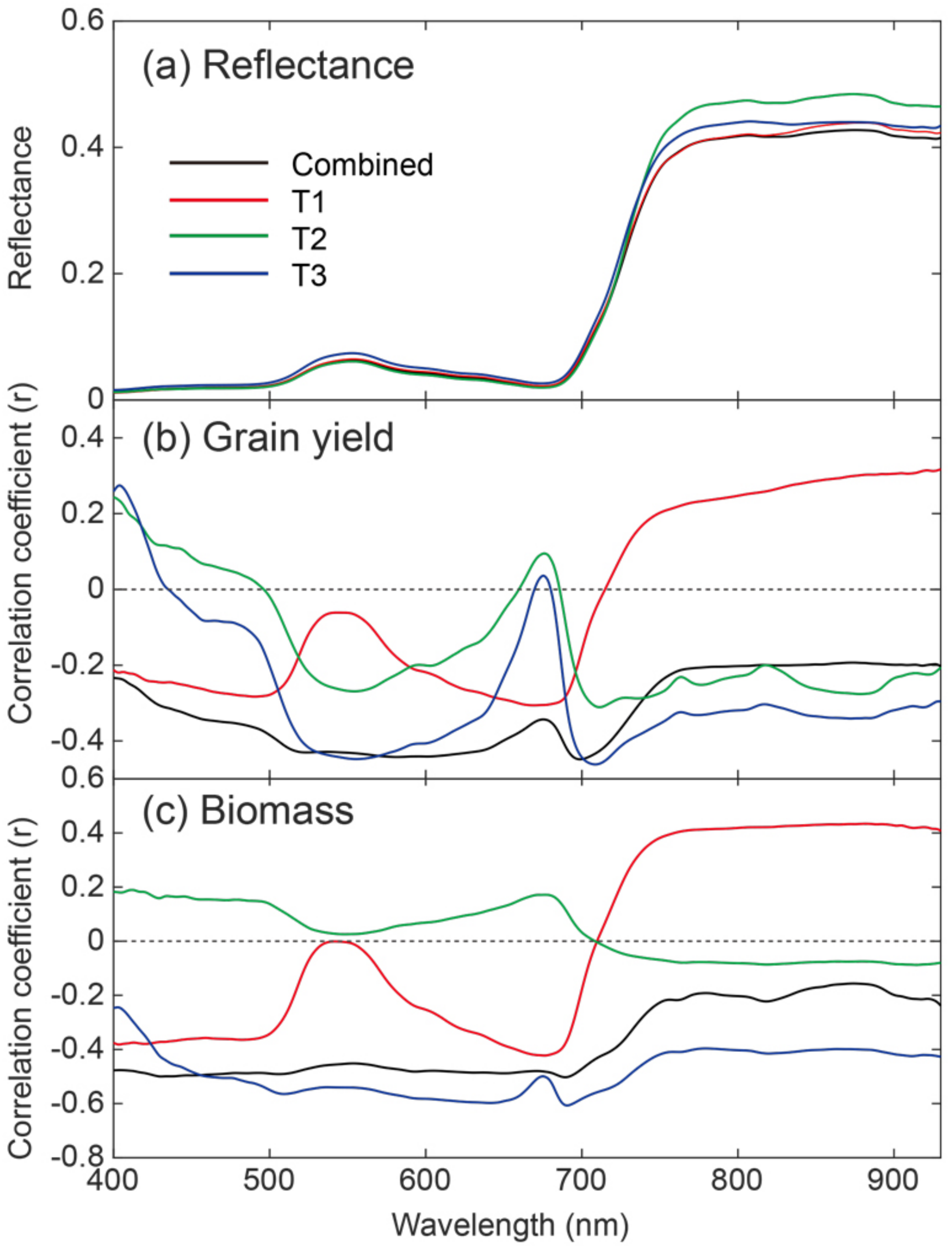
3.2. Relationships between Canopy Reflectance and Grain Yield, BM

Figure 5 shows the mean canopy reflectance and Pearson’s correlation coefficient (r) values between grain yield, BM, and reflectance spectra for the T1, T2, and T3 data sets. Differences in mean reflectance were observed mainly in the green (520–580 nm) and NIR (740–930 nm) wavelength regions. With respect to the mean reflectance at the booting stage (T2), the reflectance values in the visible regions (400–680 nm) were lower than those in the other data stages, while the values were higher in the NIR region (681–930 nm). The visible wavelength regions are related mainly to absorption by chlorophyll a (centred at 430 and 660 nm) and chlorophyll b (centred at 640 nm), while reflectance in the NIR region is determined mainly by the multiple scattering of light within the leaf due to internal leaf structure characteristics [58,59].
Regarding correlations with grain yield at the ripening stage (T1), the shape showed the opposite tendency to that shown by the other stages (Figure 5b). A similar trend was also reported by Gnyp et al. [27], who reported that the pattern of correlation curves was similar at the different stages (tillering, stem elongation, and booting stage) except for the heading stage. In the present study, the r values ranged between −0.45 and 0.35. Even though the r values were slightly insignificant, the reflectance values at 550 nm and 709–711 were highly correlated with the grain yield from the panicle initiation stage (T3) to the booting stage (T2). The 550 nm region is near the peak of green reflectance [60], whereas the 700–780 nm region is known as the red-edge region, which is strongly related to the chlorophyll concentration and has been used to assess the N status of crops [61,62,63,64]. These two spectral regions have been used because of their high sensitivity to pigment contents in various plant species [60,65]. At the ripening stage, leaf senescence that takes places in plants during seed formation is accompanied by a progressive decrease in the photosynthetic pigments.
Similar to grain yield, the shape of correlations with BM at the ripening stage (T1) showed the opposite tendency to the others (Figure 5c). Except for the booting stage (T2), the absolute r values showed relatively higher values than that shown in grain yield. This might indicate that the canopy HS reflectance was influenced by the BM more than the grain yield. Meanwhile, the canopy HS at the booting stage is less sensitive than at other stages, which might be reflected by other factors relating to the yield potential, which will be discussed more in the next section.

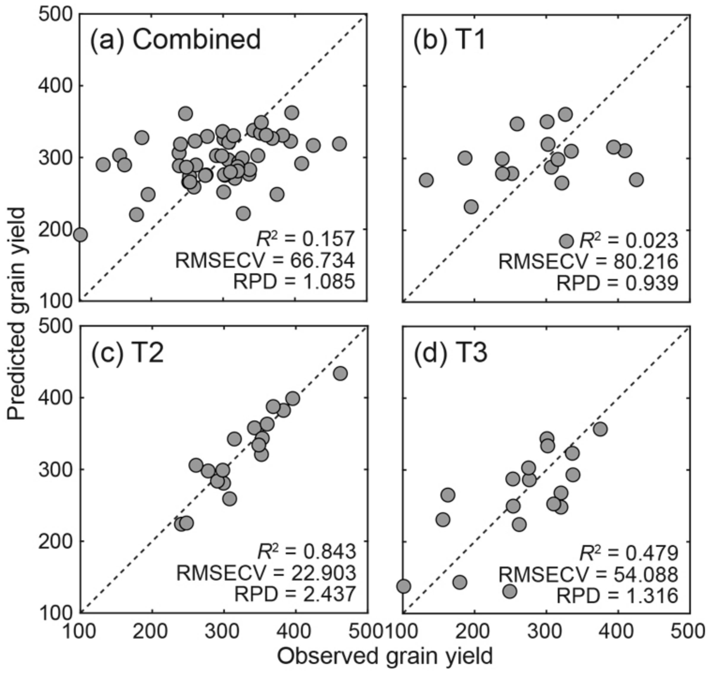
3.3. Grain Yield Evaluations with the FS-PLS and ISE-PLS Models

The cross-validated calibration results between canopy HS reflectance spectra and grain yields via FS-PLS and ISE-PLS are shown in Table 2; the selected number of wavebands (NW) and the selected NW as a percentage of the full spectrum (NW% = NW/whole waveband [531 bands] × 100) are included. The NW (NW%) ranged from 2 to131 (0.4–24.7%). The optimum NLV ranged from 1 to 10 and was determined as the lowest RMSECV values calculated from LOO cross-validation to avoid over-fitting the model. The ISE-PLS models showed better predictive accuracy than the FS-PLS models. Figure 6 shows the relationships between the observed and cross-validated prediction values of grain yield in each data set as predicted by the ISE-PLS models. These findings support previous results indicating that the performance of FS-PLS models can be improved via waveband selection [42,52].
Overall, the best R2 and lowest RMSECV values were obtained with ISE-PLS at the booting stage of the T2 data set (R2 = 0.843, RMSECV = 22.903). Moreover, low predictive accuracy from the combined data could indicate that the in-season rice yield assessment depends on the appropriate growth stage for canopy HS measurements. The RPD value indicated that the T2 data set used in the ISE-PLS model accurately predicted the rice grain yield (RPD = 2.437). Although the predictive accuracy for the T3 data set was lower, it could still be used confidently to make quantitative predictions by ISE-PLS (RPD = 1.316). These results indicated that rice yield could be evaluated from HS data of the reproductive phase, even though there were variations in the growth stage for cultivars in paddy fields. Moreover, the booting stage (prior to flowering) of T2 could be the best timing for acquiring canopy HS measurements to assess grain yield, and measurements after the flowering and heading stages of T1 might be difficult. These findings are in agreement with those of previous studies in that the booting stage may be the best time for assessing rice grain yield with remote sensing technology [66,67]. The booting stage represents the peak period of nutrient growth for rice plants and has the highest LAI, which can be attributed to the maximal photosynthetic capacity and yield potential.
The improvement in grain yield is related to both BM (dry matter accumulation) and harvest index (HI) [68], which can be explained by yield = HI × BM. Here, the relationship between canopy HS data and BM is generally site-dependent and changes over time due to the changes in specific leaf area, leaf ratio, and HI. In order to clarify the contribution of BM in yield evaluation of the present study, linear regression analysis was also performed between BM and grain yield (Figure 7). The BM at the harvest time correlated with the rice grain yield (R2 = 0.351, p < 0.01), but had a lower correlation than that of the result of canopy HS assessments using T2 data. The result confirmed that the BM was one of the parameters to assess grain yield after the heading stage, but growth and nutritive status assessed by canopy HS measurements before the heading stage were more reflective of the yield. Historically, crop physiologists have studied the importance of increased BM after the heading stage because the rice grain was determined during grain filling from heading to maturity stages [69,70]. However, recent researches clearly indicated that crop growth during the late reproductive period related to the grain yield in rice [71,72]. Takai et al. [72] stated that, even if the rice varieties differed in HI, the grain yield could be explained by the growth rate approximately two weeks before heading. Their previous knowledge supports our findings that canopy HS measurements at the booting stage is the best timing for assessing grain yield.

3.4. Important Wavebands for Predicting Rice Grain Yield

The selected wavebands from ISE-PLS with the mean reflectance spectra are shown in Figure 8. In addition, Table 3 lists the main selected wavebands found within 20 nm of known absorption features in the visible and NIR wavebands [58,61,64,73,74,75]. The red-edge (710–740 nm) wavelength region was commonly selected in the majority of the ISE-PLS models, while the wavebands in the visible region were selected in only the T3 data set (the panicle initiation stage). In the booting stage of the T2 data set, the red-edge and NIR (830 nm) wavebands were selected in the final model and exhibited good predictive accuracy.
The importance of these selected wavebands could be explained by process of N accumulation and distribution during the rice growth stages. The accumulation and distribution of N in the vegetative and reproductive organs of rice are the important processes in the determination of grain yield [76], and leaves are major storage organs for N. From mid-tillering to 10 days after panicle initiation, the period at which N uptake is maximal, 65% of the aboveground N is located within green leaf blades [77]. Besides, the red-edge region is strongly related to LAI and chlorophyll concentration, and indirectly correlated with leaf N [18]. Thus, the red-edge region was selected as having important wavebands for the final model in this study. During the grain-filling period, a large amount of N is required. The amount of N absorbed by the plant during this period is much smaller than the amount of N that accumulates in the mature grains, and a large portion of grain N is translocated from vegetative organs, especially leaf blades [78]. Therefore, canopy HS data at the ripening stage, when leaf N diminishes, is not considered a suitable period for estimating rice yield.

4. Conclusions

Timely and accurate rice yield assessments prior to harvest enable farmers and rice-processing industries to quantify the production supply and market prices. In this study, we evaluated the feasibility of using canopy HS data for in-season grain yield evaluations at the reproductive phase of rice. We also investigated the performance of the ISE-PLS model by comparing it with the standard FS-PLS model and discussed the importance of the selected wavebands for ISE-PLS.
Our results indicated that rice grain yield can be assessed by the ISE-PLS model, and the booting stage was identified as the best time for in-season evaluations via canopy HS assessments. The selected wavebands occurred in the red-edge and NIR wavelength regions. The selected wavebands in the ISE-PLS model allowed assessments of rice grain yield with 84% accuracy. These findings suggest that it is possible to evaluate rice yield from rice canopy reflectance approximately one month prior to harvest (average DTH = −30.7 days) which could be useful information not only for famers but also for rice processing industries to quantify rice supply and market prices. Moreover, the wavebands selected with ISE-PLS in the booting stage could be tested by Sentinel-2 or other sensors from space. These wavebands could also be evaluated in a rain-fed rice field by HS sensors or multi-spectral cameras onboard an unmanned aerial vehicle (UAV). Thus, the models and methods should be further examined with multi-year data sets.

Author Contributions

K.K., H.I., and S.P. designed this study; K.K., H.I., S.P., and P.K. performed the field work and carried out the field HS measurements; K.K. processed the HS data and wrote the manuscript; and all the authors revised the paper.

Funding

This study was conducted as part of a project sponsored by the Japan International Research Center for Agricultural Sciences (JIRCAS) on the “Formation of food value chain through value addition of food resources to support sustainable rural development”.

Acknowledgments

We are grateful to Naruo Matsumoto and Hidetoshi Asai of the JIRCAS, Japan, for their valuable comments. We also thank Thavone Inthavong and Mr. Soukasdachanh Souvannasing of the NAFRI, Laos, for their supports in the field experiments.

Conflicts of Interest

The authors declare no conflict of interest.

References

  1. Global Rice Science Partnership. Rice Almanac, 4th ed.; International Rice Research Institute: Los Banos, Philippines, 2013; ISBN 978-9712203008. [Google Scholar]
  2. World Bank. Lao People’s Democratic Republic Rice Policy Study; World Bank: Washington, DC, USA, 2012. [Google Scholar]
  3. Yoshida, H.; Takehisa, K.; Kojima, T.; Ohno, H.; Sasaki, K.; Nakagawa, H. Modeling the effects of N application on growth, yield and plant properties associated with the occurrence of chalky grains of rice. Plant Prod. Sci. 2016, 19, 30–42. [Google Scholar] [CrossRef] [Green Version]
  4. Ntanos, D.A.; Koutroubas, S.D. Dry matter and N accumulation and translocation for Indica and Japonica rice under Mediterranean conditions. Field Crops Res. 2002, 74, 93–101. [Google Scholar] [CrossRef]
  5. Kamiji, Y.; Yoshida, H.; Palta, J.A.; Sakuratani, T.; Shiraiwa, T. N applications that increase plant N during panicle development are highly effective in increasing spikelet number in rice. Field Crops Res. 2011, 122, 242–247. [Google Scholar] [CrossRef]
  6. Yoshida, H.; Horie, T. A process model for explaining genotypic and environmental variation in growth and yield of rice based on measured plant N accumulation. Fied Crops Res. 2009, 113, 227–237. [Google Scholar] [CrossRef]
  7. Bouman, B.A.M.; Kropff, M.J.; Tuong, T.P.; Wopereis, M.C.S.; ten Berge, H.F.M.; van Laar, H.H. Oryza2000: Modeling Lowland Rice; International Rice Research Institute and Wageningen University and Research Centre: Los Baños, Philippines, 2001; ISBN 9712201716. [Google Scholar]
  8. Inoue, Y.; Sakaiya, E.; Zhu, Y.; Takahashi, W. Diagnostic mapping of canopy nitrogen content in rice based on hyperspectral measurements. Remote Sens. Environ. 2012, 126, 210–221. [Google Scholar] [CrossRef]
  9. Nguyen, H.T.; Lee, B.-W. Assessment of rice leaf growth and nitrogen status by hyperspectral canopy reflectance and partial least square regression. Eur. J. Agron. 2006, 24, 349–356. [Google Scholar] [CrossRef]
  10. Tan, K.; Wang, S.; Song, Y.; Liu, Y.; Gong, Z. Estimating nitrogen status of rice canopy using hyperspectral reflectance combined with BPSO-SVR in cold region. Chemom. Intell. Lab. Syst. 2018, 172, 68–79. [Google Scholar] [CrossRef]
  11. Wang, L.; Zhang, F.C.; Jing, Y.S.; Jiang, X.D.; Yang, S.B.; Han, X.M. Multi-temporal detection of rice phenological stages using canopy stagespectrum. Rice Sci. 2014, 21, 108–115. [Google Scholar] [CrossRef]
  12. Yu, K.; Li, F.; Gnyp, M.L.; Miao, Y.; Bareth, G.; Chen, X. Remotely detecting canopy nitrogen concentration and uptake of paddy rice in the Northeast China Plain. ISPRS J. Photogramm. Remote Sens. 2013, 78, 102–115. [Google Scholar] [CrossRef]
  13. Hatfield, J.L.; Prueger, J.H. Value of using different vegetative indices to quantify agricultural crop characteristics at different growth stages under varying management practices. Remote Sens. 2010, 2, 562–578. [Google Scholar] [CrossRef]
  14. Atzberger, C.; Darvishzadeh, R.; Immitzer, M.; Schlerf, M.; Skidmore, A.; le Maire, G. Comparative analysis of different retrieval methods for mapping grassland leaf area index using airborne imaging spectroscopy. Int. J. Appl. Earth Obs. Geoinf. 2015, 43, 19–31. [Google Scholar] [CrossRef] [Green Version]
  15. Campbell, G.S.; Norman, J.M. The Description and Measurement of Plant Canopy Structure; Cambridge University Press: Cambridge, UK, 1989; Volume 31, pp. 1–19. [Google Scholar]
  16. Casa, R.; Varella, H.; Buis, S.; Guérif, M.; De Solan, B.; Baret, F. Forcing a wheat crop model with LAI data to access agronomic variables: Evaluation of the impact of model and LAI uncertainties and comparison with an empirical approach. Eur. J. Agron. 2012, 37, 1–10. [Google Scholar] [CrossRef]
  17. Schlemmer, M.; Gitelson, A.; Schepers, J.; Ferguson, R.; Peng, Y.; Shanahan, J.; Rundquist, D. Remote estimation of nitrogen and chlorophyll contents in maize at leaf and canopy levels. Int. J. Appl. Earth Obs. Geoinf. 2013, 25, 47–54. [Google Scholar] [CrossRef] [Green Version]
  18. Baret, F.; Houlès, V.; Guérif, M. Quantification of plant stress using remote sensing observations and crop models: The case of nitrogen management. J. Exp. Bot. 2007, 58, 869–880. [Google Scholar] [CrossRef] [PubMed]
  19. Filella, I.; Serrano, L.; Serra, J.; Peñuelas, J. Evaluating Wheat Nitrogen Status with Canopy Reflectance Indices and Discriminant Analysis. Crop Sci. 1995, 35, 1400–1405. [Google Scholar] [CrossRef]
  20. Gnyp, M.L.; Miao, Y.; Yuan, F.; Ustin, S.L.; Yu, K.; Yao, Y.; Huang, S.; Bareth, G. Hyperspectral canopy sensing of paddy rice aboveground biomass at different growth stages. Field Crops Res. 2014, 155, 42–55. [Google Scholar] [CrossRef]
  21. Yao, Y.; Miao, Y.; Huang, S.; Gao, L.; Ma, X.; Zhao, G.; Jiang, R.; Chen, X.; Zhang, F.; Yu, K.; et al. Active canopy sensor-based precision N management strategy for rice. Agron. Sustain. Dev. 2012, 32, 925–933. [Google Scholar] [CrossRef] [Green Version]
  22. Cao, Q.; Miao, Y.; Shen, J.; Yu, W.; Yuan, F.; Cheng, S.; Huang, S.; Wang, H.; Yang, W.; Liu, F. Improving in-season estimation of rice yield potential and responsiveness to topdressing nitrogen application with Crop Circle active crop canopy sensor. Precis. Agric. 2016, 17, 136–154. [Google Scholar] [CrossRef]
  23. Rouse, J.W. Monitoring Vegetation Systems in the Great Plains with ERTS; NASA: Washington, DC, USA, 1973; pp. 309–317. [Google Scholar]
  24. Jordan, J.C. Derivation of leaf-area index from quality of light on the forest floor. Ecology 1969, 50, 663–666. [Google Scholar] [CrossRef]
  25. Haboudane, D.; Miller, R.J.; Pattey, E.; Zarco-Tejada, J.P.; Strachan, B.I. Hyperspectral vegetation indices and novel algorithms for predicting green LAI of crop canopies: Modeling and validation in the context of precision agriculture. Remote Sens. Environ. 2004, 90, 337–352. [Google Scholar] [CrossRef]
  26. Thenkabail, P.S.; Smith, R.B.; De Pauw, E. Hyperspectral vegetation indices and their relationships with agricultural crop characteristics. Remote Sens. Environ. 2000, 71, 158–182. [Google Scholar] [CrossRef]
  27. Gnyp, M.L.; Yu, K.; Aasen, H.; Yao, Y.; Huang, S.; Miao, Y.; Bareth, G. Analysis of crop reflectance for estimating biomass in rice canopies at different phenological stages: Reflexions analyse zur Abschätzung der Biomasse von Reis in unterschiedlichen phänologischen Stadien. Photogramm. Fernerkundung Geoinf. 2013, 2013, 351–365. [Google Scholar] [CrossRef]
  28. Yang, C.-M.; Chen, R.-K. Modeling rice growth with hyperspectral reflectance data. Crop Sci. 2004, 44, 1283–1290. [Google Scholar] [CrossRef]
  29. Kokaly, R.F.; Clark, R.N. Spectroscopic determination of leaf biochemistry using band-depth analysis of absorption features and stepwise multiple linear regression. Remote Sens. Environ. 1999, 67, 267–287. [Google Scholar] [CrossRef]
  30. Zhao, D.; Reddy, K.R.; Kakani, V.G.; Read, J.J.; Koti, S. Selection of optimum reflectance ratios for estimating leaf nitrogen and chlorophyll concentrations of field-grown cotton. Agron. J. 2005, 97, 89–98. [Google Scholar] [CrossRef]
  31. Nguyen, H.T.; Kim, J.H.; Nguyen, A.T.; Nguyen, L.T.; Shin, J.C.; Lee, B.-W. Using canopy reflectance and partial least squares regression to calculate within-field statistical variation in crop growth and nitrogen status of rice. Precis. Agric. 2006, 7, 249–264. [Google Scholar] [CrossRef]
  32. Yu, K.; Gnyp, M.L.; Gao, L.; Miao, Y.; Chen, X.; Bareth, G. Estimate leaf chlorophyll of rice using reflectance indices and partial least squares. Photogramm.–Fernerkundung–Geoinf. 2015, 2015, 45–54. [Google Scholar] [CrossRef]
  33. Wold, S.; Sjöström, M.; Eriksson, L. PLS-regression: A basic tool of chemometrics. Chemom. Intell. Lab. Syst. 2001, 58, 109–130. [Google Scholar] [CrossRef]
  34. Hansen, P.M.; Schjoerring, J.K. Reflectance measurement of canopy biomass and nitrogen status in wheat crops using normalized difference vegetation indices and partial least squares regression. Remote Sens. Environ. 2003, 86, 542–553. [Google Scholar] [CrossRef]
  35. Fu, Y.; Yang, G.; Wang, J.; Song, X.; Feng, H. Winter wheat biomass estimation based on spectral indices, band depth analysis and partial least squares regression using hyperspectral measurements. Comput. Electron. Agric. 2014, 100, 51–59. [Google Scholar] [CrossRef]
  36. Li, F.; Mistele, B.; Hu, Y.; Chen, X.; Schmidhalter, U. Reflectance estimation of canopy nitrogen content in winter wheat using optimised hyperspectral spectral indices and partial least squares regression. Eur. J. Agron. 2014, 52, 198–209. [Google Scholar] [CrossRef]
  37. Weber, V.S.; Araus, J.L.; Cairns, J.E.; Sanchez, C.; Melchinger, A.E.; Orsini, E. Prediction of grain yield using reflectance spectra of canopy and leaves in maize plants grown under different water regimes. Field Crops Res. 2012, 128, 82–90. [Google Scholar] [CrossRef]
  38. Ryu, C.; Suguri, M.; Umeda, M. Multivariate analysis of nitrogen content for rice at the heading stage using reflectance of airborne hyperspectral remote sensing. Field Crops Res. 2011, 122, 214–224. [Google Scholar] [CrossRef] [Green Version]
  39. Kawamura, K.; Watanabe, N.; Sakanoue, S.; Lee, H.J.; Inoue, Y.; Odagawa, S. Testing genetic algorithm as a tool to select relevant wavebands from field hyperspectral data for estimating pasture mass and quality in a mixed sown pasture using partial least squares regression. Grassl. Sci. 2010, 56, 205–216. [Google Scholar] [CrossRef]
  40. Kawamura, K.; Watanabe, N.; Sakanoue, S.; Lee, H.J.; Lim, J.; Yoshitoshi, R. Genetic algorithm-based partial least squares regression for estimating legume content in a grass-legume mixture using field hyperspectral measurements. Grassl. Sci. 2013, 59, 166–172. [Google Scholar] [CrossRef]
  41. Darvishzadeh, R.; Skidmore, A.; Schlerf, M.; Atzberger, C.; Corsi, F.; Cho, M. LAI and chlorophyll estimation for a heterogeneous grassland using hyperspectral measurements. ISPRS J. Photogramm. Remote Sens. 2008, 63, 409–426. [Google Scholar] [CrossRef]
  42. Cho, M.A.; Skidmore, A.; Corsi, F.; van Wieren, S.E.; Sobhan, I. Estimation of green grass/herb biomass from airborne hyperspectral imagery using spectral indices and partial least squares regression. Int. J. Appl. Earth Obs. Geoinf. 2007, 9, 414–424. [Google Scholar] [CrossRef]
  43. Bolster, K.L.; Martin, M.E.; Aber, J.D. Determination of carbon fraction and nitrogen concentration in tree foliage by near infrared reflectance: A comparison of statistical methods. Can. J. For. Res. 1996, 26, 590–600. [Google Scholar] [CrossRef]
  44. Kawamura, K.; Watanabe, N.; Sakanoue, S.; Inoue, Y. Estimating forage biomass and quality in a mixed sown pasture based on PLS regression with waveband selection. Grassl. Sci. 2008, 54, 131–146. [Google Scholar] [CrossRef]
  45. Boggia, R.; Forina, M.; Fossa, P.; Mosti, L. Chemometric study and validation strategies in the structure-activity relationships of new cardiotonic agents. Quant. Struct. Relationsh. 1997, 16, 201–213. [Google Scholar] [CrossRef]
  46. Leardi, R.; González, A.L. Genetic algorithms applied to feature selection in PLS regression: How and when to use them. Chemom. Intell. Lab. Syst. 1998, 41, 195–207. [Google Scholar] [CrossRef]
  47. Gomez, K.A.; De Datta, S.K. Border effects in rice experimental plots I. unplanted borders. Exp. Agric. 2008, 7, 87–92. [Google Scholar] [CrossRef]
  48. Wang, K.; Zhou, H.; Wang, B.; Jian, Z.; Wang, F.; Huang, J.; Nie, L.; Cui, K.; Peng, S. Quantification of border effect on grain yield measurement of hybrid rice. Field Crops Res. 2013, 141, 47–54. [Google Scholar] [CrossRef]
  49. Tubaña, B.; Harrell, D.; Walker, T.; Teboh, J.; Lofton, J.; Kanke, Y.; Phillips, S. Relationships of spectral vegetation indices with rice biomass and grain yield at different sensor view angles. Agron. J. 2011, 103, 1405–1413. [Google Scholar] [CrossRef]
  50. Qi, J.; Chehbouni, A.; Huete, A.R.; Kerr, H.Y.; Sorooshian, S. A modified soil adjusted vegetation index. Remote Sens. Environ. 1994, 48, 119–126. [Google Scholar] [CrossRef]
  51. Savitzky, A.; Golay, M.J.E. Smoothing and differentiation of data by simplified least squares procedures. Anal. Chem. 1964, 36, 1627–1639. [Google Scholar] [CrossRef]
  52. Kawamura, K.; Tsujimoto, Y.; Rabenarivo, M.; Asai, H.; Andriamananjara, A.; Rakotoson, T. Vis-NIR spectroscopy and PLS regression with waveband selection for estimating the total C and N of paddy soils in Madagascar. Remote Sens. 2017, 9, 1081. [Google Scholar] [CrossRef]
  53. Forina, M.; Lanteri, S.; Oliveros, M.C.C.; Millan, C.P. Selection of useful predictors in multivariate calibration. Anal. Bioanal. Chem. 2004, 380, 397–418. [Google Scholar] [CrossRef] [PubMed]
  54. Mevik, B.-H.; Cederkvist, H.R. Mean squared error of prediction (MSEP) estimates for principal component regression (PCR) and partial least squares regression (PLSR). J. Chemom. 2004, 18, 422–429. [Google Scholar] [CrossRef]
  55. Williams, P.C. Implementation of near-infrared technology. In Near-Infrared Technology in the Agricultural and Food Industries; Williams, P.C., Norris, K.H., Eds.; American Association of Cereal Chemists Inc.: St. Paul, MN, USA, 2001; pp. 145–169. [Google Scholar]
  56. D’Acqui, L.P.; Pucci, A.; Janik, L.J. Soil properties prediction of western Mediterranean islands with similar climatic environments by means of mid-infrared diffuse reflectance spectroscopy. Eur. J. Soil Sci. 2010, 61, 865–876. [Google Scholar] [CrossRef]
  57. Zhao, H.; Fu, Y.H.; Wang, X.; Zhao, C.; Zeng, Z.; Piao, S. Timing of rice maturity in China is affected more by transplanting date than by climate change. Agric. For. Meteorol. 2016, 216, 215–220. [Google Scholar] [CrossRef]
  58. Curran, P. Remote sensing of foliar chemistry. Remote Sens. Environ. 1989, 30, 271–278. [Google Scholar] [CrossRef]
  59. Curran, P.; Dungan, J.; Peterson, D. Estimating the foliar biochemical concentration of leaves with reflectance spectrometry Testing the Kokaly and Clark methodologies. Remote Sens. Environ. 2001, 76, 349–359. [Google Scholar] [CrossRef]
  60. Gitelson, A.A.; Kaufman, Y.J.; Merzlyak, N.M. Use of a green channel in remote sensing of global vegetation from EOS-MODIS. Remote Sens. Environ. 1996, 58, 289–298. [Google Scholar] [CrossRef]
  61. Horler, H.N.D.; Dockray, M.; Barber, J. The red edge of plant leaf reflectance. Int. J. Remote Sens. 1983, 4, 273–288. [Google Scholar] [CrossRef]
  62. Kanke, Y.; Tubaña, B.; Dalen, M.; Harrell, D. Evaluation of red and red-edge reflectance-based vegetation indices for rice biomass and grain yield prediction models in paddy fields. Precis. Agric. 2016, 17, 507–530. [Google Scholar] [CrossRef]
  63. Evri, M.; Akiyama, T.; Kawamura, K. Spectrum analysis of hyperspectral red edge position to predict rice biophysical parameters and grain weight. J. Jpn. Soc. Photogramm. Remote Sens. 2008, 47, 4–15. [Google Scholar] [CrossRef] [Green Version]
  64. Peñuelas, J.; Gamon, J.A.; Fredeen, A.L.; Merino, J.; Field, C.B. Reflectance indices associated with physiological changes in nitrogen- and water-limited sunflower leaves. Remote Sens. Environ. 1994, 48, 135–146. [Google Scholar] [CrossRef]
  65. Gitelson, A.; Merzlyak, M.N. Spectral relfectance changes associated with autumn senescence of Aesculus hippocastanum L. and Acer platanoides L. leaves. Spectral features and relation to chlorophyll estimation. J. Plant Physiol. 1994, 143, 286–292. [Google Scholar] [CrossRef]
  66. Chang, K.-W.; Shen, Y.; Lo, J.-C. Predicting rice yield using canopy reflectance measured at booting stage. Agron. J. 2005, 97, 872–878. [Google Scholar] [CrossRef]
  67. Zhou, X.; Zheng, H.B.; Xu, X.Q.; He, J.Y.; Ge, X.K.; Yao, X.; Cheng, T.; Zhu, Y.; Cao, W.X.; Tian, Y.C. Predicting grain yield in rice using multi-temporal vegetation indices from UAV-based multispectral and digital imagery. ISPRS J. Photogramm. Remote Sens. 2017, 130, 246–255. [Google Scholar] [CrossRef]
  68. Peng, S.; Laza, R.C.; Visperas, R.M.; Sanico, A.L.; Cassman, K.G.; Khush, G.S. Grain yield of rice cultivars and lines developed in the Philippines since 1966. Crop Sci. 2000, 40, 307–314. [Google Scholar] [CrossRef]
  69. Murchie, E.H.; Yang, J.; Hubbart, S.; Horton, P.; Peng, S. Are there associations between grain-filling rate and photosynthesis in the flag leaves of field-grown rice? J. Exp. Bot. 2002, 53, 2217–2224. [Google Scholar] [CrossRef] [PubMed] [Green Version]
  70. Saitoh, K.; Shimoda, H.; Ishihara, K. Characteristics of dry matter production process in high-yield rice varieties: VI. Comparisons between new and old rice varieties. Jpn. J. Crop Sci. 1993, 62, 509–517. [Google Scholar] [CrossRef]
  71. Horie, A.; Isono, K.; Koseki, H. Generation of a monoclonal antibody against the mouse Sf3b1 (SAP155) gene product for U2 snRNP component of spliceosome. Hybrid. Hybrid. 2003, 22, 117–119. [Google Scholar] [CrossRef] [PubMed]
  72. Takai, T.; Matsuura, S.; Nishio, T.; Ohsumi, A.; Shiraiwa, T.; Horie, T. Rice yield potential is closely related to crop growth rate during late reproductive period. Field Crops Res. 2006, 96, 328–335. [Google Scholar] [CrossRef]
  73. Ben-Dor, E.; Inbar, Y.; Chen, Y. Reflectance spectra of organic matter in the visible near-infrared and short wave infrared region (400–2500 nm) during a controlled decomposition process. Remote Sens. Environ. 1997, 61, 1–15. [Google Scholar] [CrossRef]
  74. Dawson, T.P.; Curran, P.J.; North, P.R.J.; Plummer, S.E. The propagation of foliar biochemical absorption features in forest canopy reflectance: A theoretical analysis. Remote Sens. Environ. 1999, 67, 147–159. [Google Scholar] [CrossRef]
  75. Elvidge, D.C. Visible and near infrared reflectance characteristics of dry plant materials. Int. J. Remote Sens. 1990, 11, 1775–1795. [Google Scholar] [CrossRef]
  76. Guindo, D.; Wells, B.R.; Wilson, C.E.; Norman, R.J. Seasonal accumulation and partitioning of nitrogen-15 in rice. Soil Sci. Soc. Am. J. 1992, 56, 1521–1527. [Google Scholar] [CrossRef]
  77. Ladha, J.K.; Kirk, G.J.D.; Bennett, J.; Peng, S.; Reddy, C.K.; Reddy, P.M.; Singh, U. Opportunities for increased nitrogen-use efficiency from improved lowland rice germplasm. Field Crops Res. 1998, 56, 41–71. [Google Scholar] [CrossRef]
  78. Mae, T. Physiological nitrogen efficiency in rice: Nitrogen utilization, photosynthesis, and yield potential. Plant Soil 1997, 196, 201–210. [Google Scholar] [CrossRef]
Figure 1. Location of the experimental field at the Rice Research Center (RRC) of the National Agriculture and Forestry Research Institute (NAFRI), and the plot design. V1–V6: Rice varieties (TDK8, TDK11, TSN7, HSV, KPB, and KKK); R1–R3: Three replicates; T1–T3: Transplanting date (12, 26 July and 9 August 2017); DAT: Days after transplanting until the canopy reflectance measurement on 2 October 2017.
Remotesensing 10 01249 g001
Figure 2. Transplanting, flowering, and harvest dates of rice for each single plot in the experimental field.
Remotesensing 10 01249 g002
Figure 3. Days to flowering (DTF) and days to harvest (DTH) from the date of field hyperspectral (HS) measurements on 2 October 2017.
Remotesensing 10 01249 g003
Figure 4. Flowchart depicting a general overview of the methodology.
Remotesensing 10 01249 g004
Figure 5. Mean canopy reflectance (a) and correlation coefficient (r) between the grain yield (b), biomass (BM) (c) and reflectance at each waveband for the T1, T2, and T3 data sets.
Remotesensing 10 01249 g005
Figure 6. Observed and cross-validated predicted values of rice grain yield (ad) using ISE-PLS regression for the combined (n = 54) and T1, T2 and T3 data sets (n = 18), respectively (see Table 2).
Remotesensing 10 01249 g006
Figure 7. Relationship between BM and grain yield.
Remotesensing 10 01249 g007
Figure 8. Canopy reflectance and selected wavebands (red bars) in the ISE-PLS models for the (a) combined (n = 54) and (b) T1, (c) T2, and (d) T3 data sets (n = 18 per transplanting date).
Remotesensing 10 01249 g008
Table 1. Descriptive statistics of rice grain yield (g m−2).
Data SetnMinMaxMeanSDCV
Combined54101.3462.0295.373.124.8
T118133.0425.6292.977.526.5
T218240.7462.0327.956.817.3
T318101.3375.1265.072.927.5
n, number of samples; SD, standard deviation; CV; coefficient of variation (= Mean/SD × 100%).
Table 2. Optimum number of latent variables (NLV), coefficient of determination (R2), root mean squared errors of cross-validation (RMSECV), and residual predictive values (RPD) from full-spectrum partial least squares (FS-PLS) and iterative stepwise elimination PLS (ISE-PLS) models with a selected number of wavebands (NW) and their percentages of the full spectrum (NW%).
Data SetRegressionNLVR2RMSECVRPDNWNW%
CombinedFS-PLS30.11368.9271.050
ISE-PLS20.15766.7341.08520.4
T1FS-PLS10.00986.1140.875
ISE-PLS20.02380.2160.9398415.8
T2FS-PLS30.07858.4800.944
ISE-PLS100.84322.9032.437112.1
T3FS-PLS80.30166.4181.068
ISE-PLS70.47954.0881.31613124.7
Bold font represents RPD > 2.0.
Table 3. Selected wavebands from the iterative stepwise elimination partial least squares (ISE-PLS) model to predict grain yield via previously known absorption features in the visible and near-infrared (NIR) wavelengths.
Previously Known Wavebands with Related Biochemical ComponentsWaveband Selected in the Present Study from ISE-PLS
Wavelength (nm)Biochemical ComponentsReferencesCombinedT1T2T3
430Chlorophyll a58, 64400, 411, 412, 433
--588–596
640Chlorophyll b58, 64643–649
660Chlorophyll a58, 64, 73690–694
700–780Chlorophyll61714723–749706, 708, 712, 717, 719, 736, 740, 741, 744731, 732, 747–762, 777–804
800Lignin, Tannin74813, 820809–813
--818–842, 861–866, 890
910Protein58, 75893–910
930Water, starch58, 75927874–930924, 926, 927, 929, 930

