Article

Ocean Wave Measurement Using Short-Range K-Band Narrow Beam Continuous Wave Radar

1
Faculty of Engineering and Applied Science, Memorial University, St. John’s, NL A1B 3X5, Canada
2
MARUM, University of Bremen, 28359 Bremen, Germany
3
Department of Physics and Physical Oceanography, Memorial University, St. John’s, NL A1B 3X7, Canada
*
Author to whom correspondence should be addressed.
Remote Sens. 2018, 10(8), 1242; https://doi.org/10.3390/rs10081242
Submission received: 11 June 2018 / Revised: 31 July 2018 / Accepted: 1 August 2018 / Published: 7 August 2018
(This article belongs to the Special Issue Ocean Radar)

Abstract

:
We describe a technique to measure ocean wave period, height and direction. The technique is based on the characteristics of transmission and backscattering of short-range K-band narrow beam continuous wave radar at the sea surface. The short-range K-band radar transmits and receives continuous signals close to the sea surface at a low-grazing angle. By sensing the motions of a dominant facet at the sea surface that strongly scatters signals back and is located directly in front of the radar, the wave orbital velocity can be measured from the Doppler shift of the received radar signal. The period, height and direction of ocean wave are determined from the relationships among wave orbital velocity, ocean wave characteristics and the Doppler shift. Numerical simulations were performed to validate that the dominant facet exists and ocean waves are measured by sensing its motion. Validation experiments were conducted in a wave tank to verify the feasibility of the proposed ocean wave measurement method. The results of simulations and experiments demonstrate the effectiveness of the short-range K-band narrow beam continuous wave radar for the measurement of ocean waves.

Graphical Abstract

1. Introduction

There are two general approaches for the measurement of ocean waves: in situ and remote sensing measurements. The in situ measurements are usually made with the instrument located in the proximity of the site of interest and typically produces a more accurate local result. For example, motion and attitude sensors mounted on a wave rider buoy [1], moored at the sea surface, detect local wave motions. Acoustic and pressure sensors fixed below the sea surface measure distance to the surface and water pressure to detect wave elevation; radar and laser wave sensors mounted above the surface look downward observing wave elevation by measuring the distance to the surface [2]. Remote sensing is conducted at a location distant from sea surface. HF radar [3,4,5,6] is employed to measure the sea wave spectrum, wave height, wind field, and surface current velocity. Both non-coherent and coherent microwave radars have been used to measure wave spectra and estimate wave characteristics at sea surface [7,8,9,10]. ISR CORrad Digital Imaging Radar [11] and Sigma S6 WaMoS II Wave Radar [12] are two commercially available X-band marine radars for which the wave measurements are based on the analysis of various radar images. Synthetic-aperture radar employs L-band and C-band to measure directional and power spectra of wave fields with interferometric configuration [13] and measure near-surface ocean currents with the phase difference between Synthetic-aperture radar image scenes [14]. Airborne Ku-band and L-band wave spectrometers were developed to measure ocean wave spectra [15]. Here, we propose a new approach to measure ocean waves with a short-range K-band narrow beam continuous wave radar (NBCWR) deployed on a surface platform. Its detection range is just tens of meters, shorter than most of the wavelengths of sea swells. Therefore a short-range K-band NBCWR is not able to scan the sea surface to generate large-area radar images covering long ocean waves. The innovation here is that ocean waves are measured by sensing the motions of a relatively small facet with a short-range K-band NBCWR at a low-grazing angles. The preliminary research on the measurement method was presented in [16]. A more detailed description and the follow-up developed research works are presented in this paper.
Due to strong atmospheric attenuation, K-band (18~27 GHz) radar is generally used for short-range applications, such as vehicle navigation and traffic supervision [17]. While restricted in range, K-band radar does exhibit great sensitivity and resolution. In this research, we use short-range K-band NBCWR for three reasons. First, K-band radar is very sensitive to wind-generated capillary waves because of the short wavelength (~1 cm). Second, the narrow beam enables the radar to transmit and receive in a specific direction such that the detected velocities can be considered as the components along the direction. Third, since the wave motions are derived from the Doppler effect [18], the radar needs to transmit a continuous wave with constant amplitude and frequency to continuously detect the Doppler shift frequency at very high resolution. Further advantages of short-range K-band NBCWR are their affordability and small size. Therefore, a short-range K-band NBCWR is used to sense the motions of a small facet of the sea surface to measure ocean wave characteristics.
The K-band radar is typically located close to the sea surface, transmitting energy at a low-grazing angle. The transmitted power and the received power are within the narrow beam antenna pattern of the radar transceiver. With these configurations and properties of the radar, a small facet at the sea surface close to, and directly in front of, the radar scatters the strongest power back to the radar transceiver. The facet is smaller than gravity waves so that the points on the facet orbit in nearly identical orbital velocities and, furthermore, the facet can also produce Bragg or breaking wave scattering because it is much greater than the radar wavelength. The facet is referred to as dominant facet and denoted by F 0 . Using numerical simulations, a typical narrow beam antenna pattern of short-range K-band NBCWR and a mathematical model of the radar cross-section (RCS) at the sea surface are implemented to calculate the received power at the radar transceiver. It is found that the received power is dominated by a facet F 0 at the sea surface which is close to, and directly in front of, the radar. The dominant facet F 0 oscillates with wave propagation. The wave orbital velocity can be measured through analysis of the Doppler shift frequency caused by the dominant facet. The period, height, and direction of the ocean waves are measured through the deterministic relationships between wave orbital velocity, ocean wave characteristics, and Doppler shift. We evaluated the proposed wave measurement method with wave tank experiments as well.

2. Methodology

2.1. Radar Signals and Dominant Facet

The short-range K-band NBCWR works with three primary radar signals: transmitted signal S T ( t ) , received signal S R ( t ) , and radar intermediate frequency (IF) output signal S I F ( t ) . They can be represented by the following three equations, respectively:
S T ( t ) = 2 P T R T s i n ( 2 π f T t ) ,
S R ( t ) = 2 P R R R s i n ( 2 π ( f T + f d ) t + φ ) ,
S I F ( t ) = 2 P I F R I F [ c o s ( 2 π f d t + φ ) + i s i n ( 2 π f d t + φ ) ] ,
where P T is the transmission power, R T is the impedance of the transmitter, P R is the received power at the radar receiver, R R is the impedance of the receiver, f d is the Doppler shift frequency, φ is the signal phase. P I F is the output power of the IF signal, and R I F is the impedance of the IF output.
In comparison with the transmitted signal, the received signal is shifted in frequency and phase, and attenuated in power, but its center frequency f T remains unchanged. The received signal is amplified and then mixed with a portion of the transmitted signal to create the complex IF signal in which only the Doppler shift frequency component f d is kept, and the power of the IF signal can be expressed by the following equation [19]:
P I F = P T G T G R σ λ 2 ( 4 π ) 3 R 4 ,
where G T is the gain of radar transmitter, G R is the gain of radar receiver, σ is the sea surface RCS, λ is the wavelength of the continuous radar wave, and R is the range to the scattering area. P T , G T , G R , and λ are the inherent properties of the radar, σ is the property of the sea surface, and R is related to the relative position of the scattering area to the radar.
If the short-range K-band NBCWR is set close to the sea surface and transmits at low-grazing angle, a dominant facet F 0 will form and it dominates the backscattered power to the radar. The formation of the dominant facet is due to the narrow radar beam width in the azimuth and a sharp attenuation in the sea surface RCS for a low-grazing K-band radar. The narrow radar beam in the azimuth concentrates the radar’s transmission and reception at a small angle, and the sharp attenuation of RCS ensures that the near surface scatters much higher power back to radar than the far surface. The radar’s low height can reduce the size of the dominant facet. Its size is much smaller than the gravity waves so that it can be considered as a surface object moving with orbital motion of the gravity waves and, furthermore, it is much greater than the radar wavelength so that it can produce Bragg or breaking wave scattering. The orbital motions of the dominant facet cause the Doppler shift frequency f d which can be obtained through analyzing the spectrogram of the continuous IF outputs. The period and the amplitude of the Doppler shift frequency variation are related to the wave period, height, and direction.

2.2. Measurement of Wave Period, Height and Direction

Wave measurement by measuring the orbital motions of gravity waves using X-band radar (8~12 GHz) has already been conducted [7,11]. Here, the relationship among the wave orbital velocity, ocean wave characteristics, and Doppler shift frequency is elaborated with the orbital motions of the dominant facet. If T , H , and α denote the wave period, height, and direction, respectively, and suppose v w is the wave orbital velocity, the three relationships are conceptually given as γ 1 :   T ,   H ,   α   v w , γ 2 :   v w f d   , and γ 3 :   f d   T ,   H ,   α , and illustrated in Figure 1.
Theoretically, γ 1 is defined by linear wave theory and γ 2 through the Doppler effect. γ 3 is consequently deduced from γ 1 and γ 2 . These relationships suggest that ocean wave characteristics can be obtained from the deterministic relationship for γ 3   if the Doppler shift frequency f d is measured.
The relationship for γ 1 is discussed first. On the basis of linear wave theory [20], the orbit of the orbital motion of ocean wave is circular in deep water or elliptical in intermediate and shallow waters. The wave orbital velocity v w can be decomposed into a horizontal component v x and a vertical component v z :
v x = π H T [ cosh k ( d + z ) sinh k d ] cos ( k x ω t ) ,
v z = π H T [ sinh k ( d + z ) sinh k d ] sin ( k x ω t ) ,
where, k is the wave number, d is the water depth, ω is the wave angular frequency and equal to 2 π / T , x is the horizontal coordinate, z is the vertical coordinate, and t is the time. v x points toward the wave direction α and v z is vertically upward. Equations (5) and (6) express the relationship γ 1 . The velocity components v x and v z can be approximately calculated by setting the coordinates x and z to a fixed point in the orbit [21]. Therefore, given H, T, k, d, and ω , and assuming the coordinates x and z to be the mean position ( x 0 , z 0 ) of the orbit, Equations (5) and (6) become periodic cosine and sine functions of time t with period of T .
Figure 2 illustrates a dominant facet F 0 (black dot) that is formed in the radiation of a short-range K-band NBCWR and traveling in a clockwise circle along with a long surface wave which propagates from left to right. The radar grazing angle is θ g . The radial velocity to the radar, v L O S , is the vector projection of wave orbital velocity v w on the radar line of sight (LOS) and can be calculated as:
v L O S = π H T [ cosh k ( d + z 0 ) sinh k d ] c o s ( k x 0 ω t θ g ) ,
Equation (7) is similar to Equation (5) except for the constant values x 0 and z 0 , and the phase difference θ g between v x and v L O S . Furthermore, supposing that θ g is a constant, v L O S is also a periodic cosine function with period of T . If a continuous radar signal with a stable frequency f T is transmitted to the dominant facet F 0 along the radar LOS, the Doppler effect modifies the continuous wave, and the Doppler shift frequency f d is calculated with:
f d = 2 f T v L O S c = 2 π f T H c T [ cosh k ( d + z 0 ) sinh k d ] cos ( k x 0 ω t θ g ) ,
where c is the speed of light. f d   is proportional to the radial velocity v L O S , so f d can also be expressed by a periodic cosine function with period of T and the term before the cos notation is the amplitude of the cosine function. Equation (8) expresses the relationship for γ 2 .
According to the relationships γ 1 and γ 2 , we know that the wave period coincides with the periods of radial velocity v L O S and Doppler shift frequency f d :
T = T L O S = T d ,
where T L O S is the period of radial velocity v L O S , and T d is the period of the Doppler shift frequency variation. The Doppler shift frequency reaches its amplitude as the dominant facet F 0 moving along the LOS, i.e., cos ( k x 0 ω t θ g ) = 1 . Therefore, the wave height can be deduced from Equation (8) and calculated from:
H = A d c T 2 π f T [ sinh k d cosh k ( d   +   z 0 ) ] ,
where A d is the amplitude of the Doppler shift frequency variation. In Equation (10), T has the measured value from Equation (9), k = 2 π / L , and the wavelength L is calculated with dispersion relation for ocean waves [22]. Equations (9) and (10) express the relationship for γ 3 . Consequently, the wave height T and wave period H are obtained through measuring the period T d and the amplitude A d of the Doppler shift frequency variation. The Doppler shift frequency can be measured by sensing the orbital motion of the dominant facet F 0 at the sea surface with the short-range K-band NBCWR which functions as a super heterodyne radar [23].
The measured wave period is considered as the true value because the period of orbital motion does not change in the radar view even if the radar is not transmitting along the wave direction. However, the measured wave height is not necessarily the true value because the angle between the wave direction and radar looking direction (here referred to as angle to the wave, β ) will affect the wave height estimation. In Equation (10), the measured amplitude A d of the Doppler shift frequency variation decreases with the coefficient | cos ( β ) | . In practice, the wave direction α and the angle to the wave β are unknown. This problem can be solved using the geometrical relationship between the true value and the several measured values. Figure 3 shows an example of the geometrical relationship for three measured wave heights.
Three vectors can be illustrated for three different magnitudes H 1 , H 2 , and H 3 and measurement directions. The three created vectors H 1 , H 2 , and H 3 are the true wave height projections in the measurement directions. By combining the three vectors at point A and constructing three perpendiculars at the end of each vector, the intersection point B is determined. The length of the line segment AB is the true value of wave height and the wave direction runs from point A to point B or the reverse. The angles β 1 , β 2 , and β 3 between line segment AB and the three vectors are also measured, respectively. The wave direction α is the angle between line segment AB and the north. In practice, a more precise result can be produced if more measured wave heights are applied.

2.3. Multiple Ocean Waves

In reality, many waves are simultaneously present at the sea surface traveling with different periods, heights, and directions. The orbital motion of the dominant facet F 0 depends on the propagation of all the waves. The wave orbital velocity v w is:
v w = n = 1 N v n ,
where v n is a velocity component which originates from the nth ocean wave, and N is the number of ocean waves. Therefore, the radial velocity to the radar v L O S and the Doppler shift frequency f d are calculated as:
v L O S = n = 1 N v n L O S ,
f d = 2 f T n = 1 N v n L O S c = n = 1 N f n d ,
where v n L O S is the radial velocity of component v n to radar, and f n d is the nth Doppler shift frequency component. Equation (13) implies that f d results from the sum of all the radial velocities and contains different frequency components, i.e., f d is the linear combination of a set of periodic cosine functions of different periods T d and amplitudes A d . It is known that the periods and the amplitudes can be demonstrated through analyzing the spectrum of f d . According to Equation (9), the resultant periods are the wave periods. Meanwhile, wave height can be calculated by Equation (10) for each wave.

3. Numerical Simulations

The measurement method is first validated via numerical simulations. The important thing is to prove that a dominant facet exists at the sea surface when the K-band NBCWR transmits and receives signals close to sea surface at low-grazing angle. Due to the short detection range, the length and width of the wave field are limited within a few hundred meters. In order to describe the orbital motion of the gravity wave and emphasize that the measurement method is based on sensing a small dominant facet at the sea surface, we use a regular wave in the wave field which is generated using the spectral peak in the Pierson-Moskowitz spectrum [24]. Each facet in the wave field scatters energy back to the radar. The received power from each facet can be calculated using Equation (4) in which the antenna pattern gains and the sea surface RCS for the K-band radar are two important parameters. In the numerical simulations, we use the typical antenna pattern gains of a K-band radar transceiver module and the calculated K-band RCS for Bragg backscattering. Through calculating the IF power received from each facet in the wave field and comparing the powers of all facets, we find that the dominant facet exists and oscillates with wave propagations.
The time series of Doppler shift frequency caused by the motions of the dominant facet can be identified and extracted from spectrogram of IF signals. We can find significant peaks in the amplitude spectrum of the time series of Doppler shift frequency. The amplitude spectrum is calculated using Fourier Transforms. Each peak gives two values: T d and A d . Consequently, the wave period and height are obtained by substituting these two values into Equations (9) and (10). Different wave heights can be measured if different radar looking directions are used. The true wave height is retrieved according to the method shown in Figure 3, in which wave direction is also measured. All the details of the process of the numerical simulations will be described in the following sub-sections.

3.1. Wave Field

By collecting the data of surface waves under differing wind conditions, the ocean wave spectra were established to describe the wave energy distribution for different wave frequencies. The Pierson-Moskowitz spectrum, which defines a wave spectrum for a fully developed sea, is given by:
S ( f ) = α 0 g 2 ( 2 π ) 4 f 5 e x p [ 0.74 ( g 2 π f U ) 4 ] ,
where f is wave frequency, α 0 is equal to 8.1 × 10⁻³, g is the gravitational acceleration, and U is the wind speed at an elevation of 19.5 m above sea surface. The significant wave height H s and the wave frequency at the spectral peak f p can be deduced with Equation (14) and expressed by the following equations:
H s 0.21 U 2 g   and   f p 0.877 g 2 π U ,
Table 1 shows the characteristics of ocean waves at the spectral peaks under wind conditions from 8–18 m/s. The wavelength L p is calculated with dispersion relation for deep water (d = 1000 m). The wave at the spectral peak is dominant because it has more energy than the others. The dominant wave generated by the 8 m/s wind is used first. 
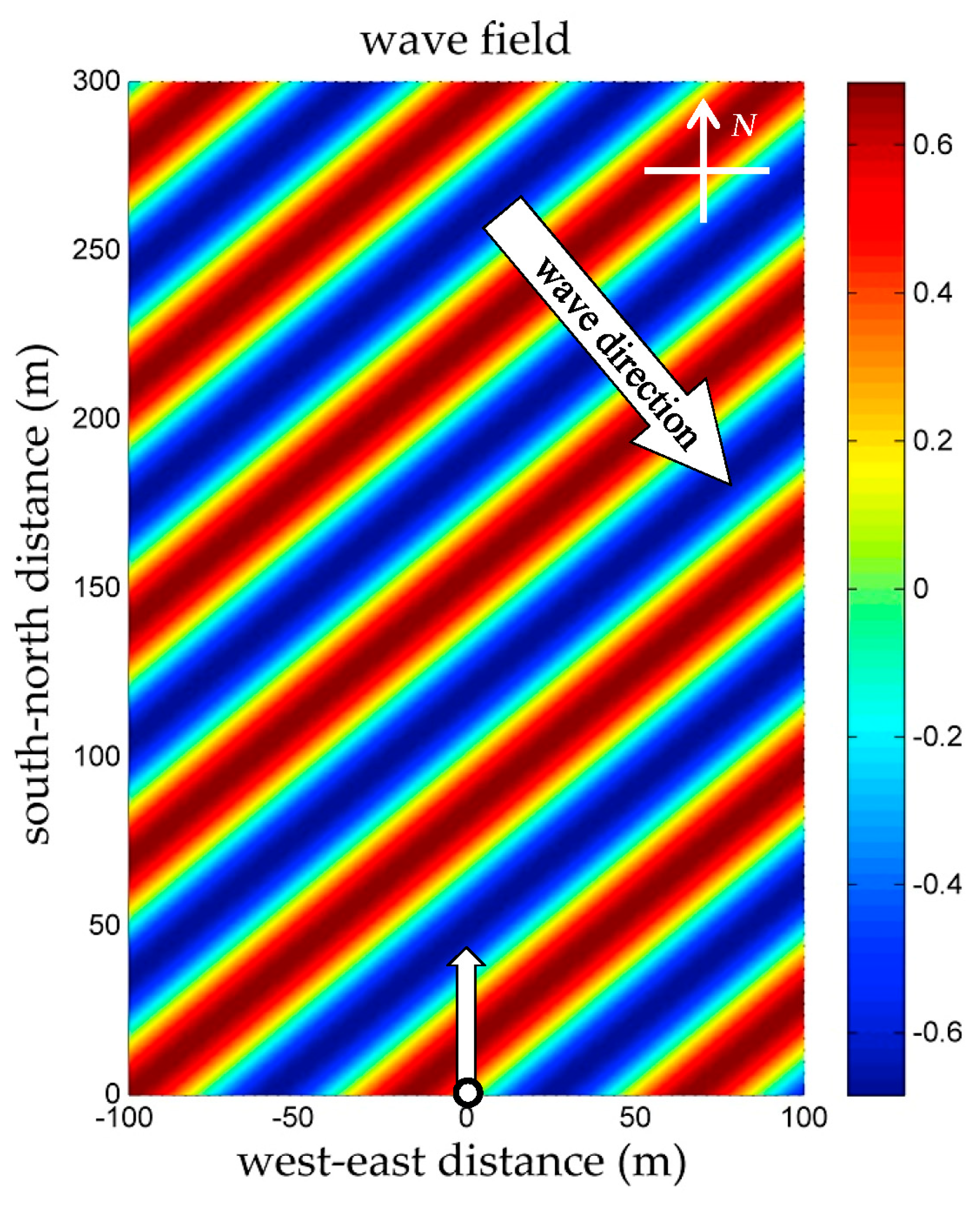
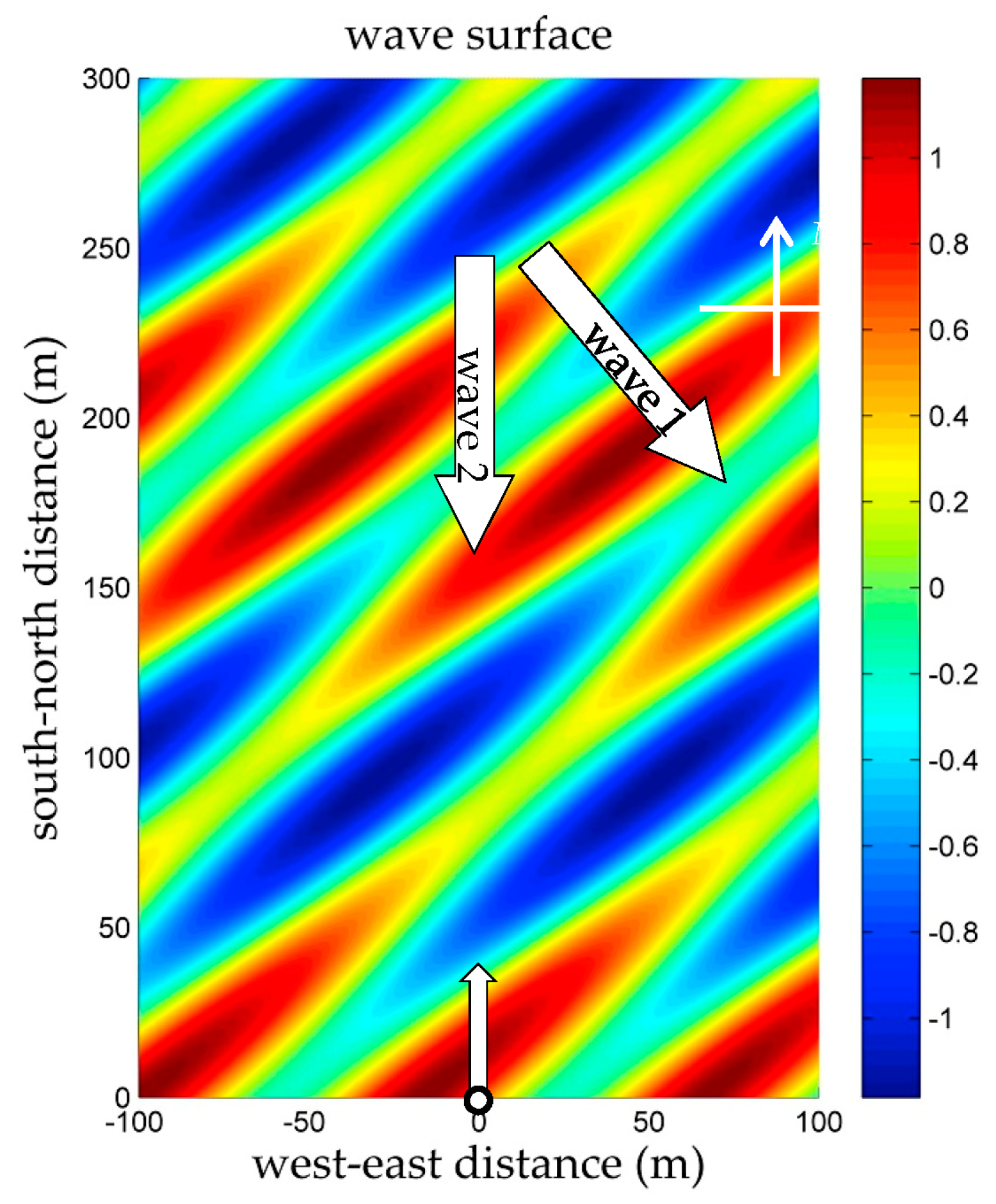
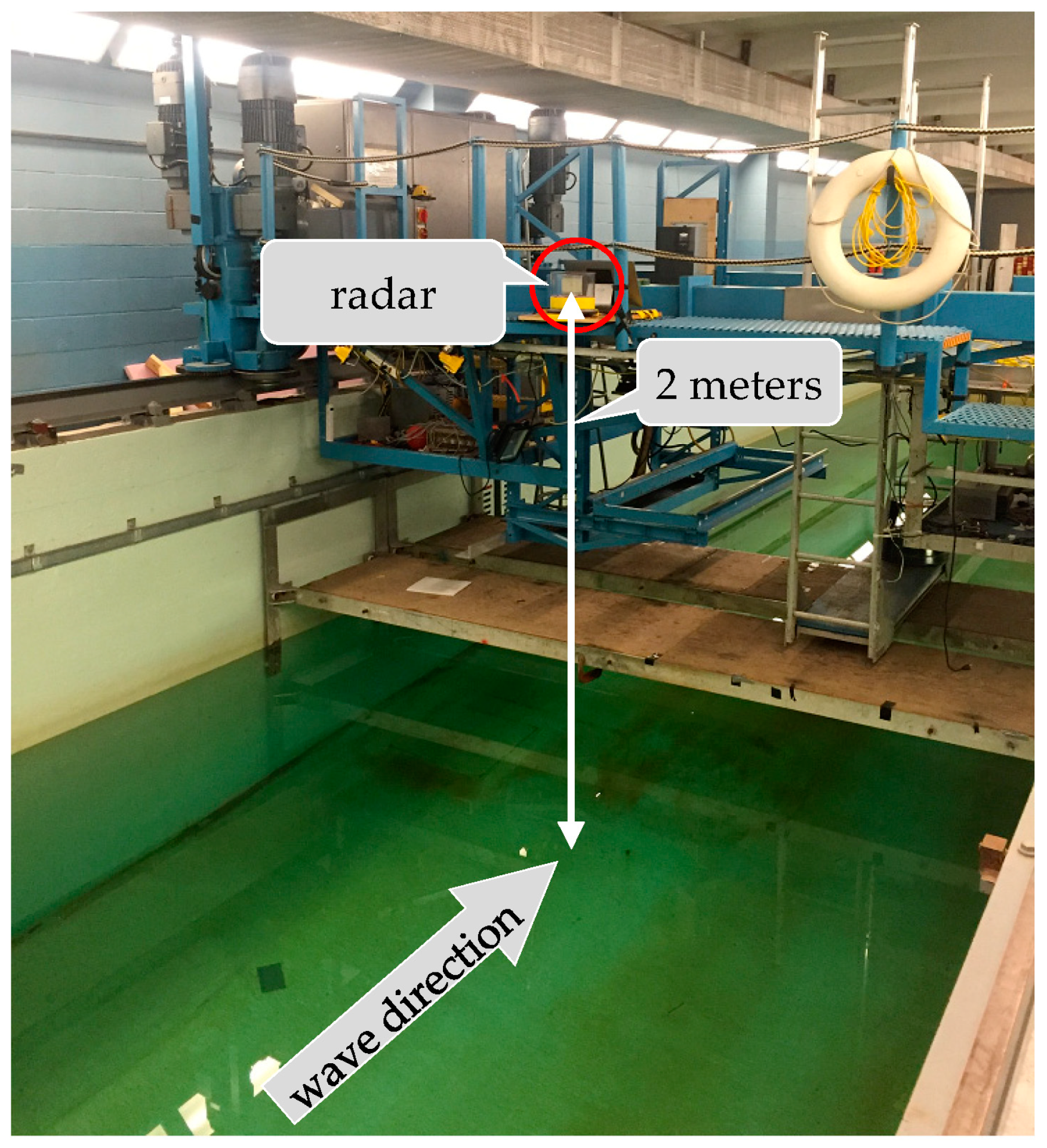
Figure 4 shows the wave field with the generated ocean waves.
The modeled sea surface size is 200 m × 300 m, and the unit facet size is 1 m × 1 m. The wave is propagating towards 140 degrees, indicated with the upper arrow. The colored stripes reveal the waveform. The radar transceiver is set 2 m above the sea level and horizontally points to the north. The small black circle at (0, 0) is its location and the lower arrow indicates the direction of the radar transceiver. Each facet is much smaller than the waves and the orbital velocities of the points in one facet are nearly identical. In addition to the waves shown in the wave field, there are also wind-generated capillary waves which are not shown in the wave field but generate backscatter. Therefore, the facets at the surface are not only orbiting with the gravity waves but also scattering radar signals back to the radar. The impacts of capillary waves will be incorporated in the calculation of RCS of sea surface.

3.2. Radar IF Output Signal

The IF output signal is regarded as the sum of all the IF components that are received from all facets at the sea surface in Figure 4 and already processed through the radar transceiver. The IF component from each facet is given by Equation (3). The Doppler shift frequency f d can be calculated by Equation (8). It should be noted that the angle to wave β must be included in the calculation. The phases of incidence and scattered waves in a single facet have possible values ranging from 0 to 2 π since the radar wavelength λ is much less than the facet size. Therefore, the phase φ of each IF component from one facet has a random value in [0, 2 π ]. The power of the IF component is calculated using the radar power equation, expressed by Equation (4).
The radar transmitter gain G T is the antenna pattern gains, while the radar receiver gain G R is composed of the global antenna gain, the amplifier gain and the antennae pattern gains [25]. They are expressed as:
G T ( θ a , θ e ) = G p a ( θ a ) + G p e ( θ e ) ,
G R ( θ a , θ e ) = G p a ( θ a ) + G p e ( θ e ) + G a n + G a m ,
where G T ( θ a , θ e ) and G R ( θ a , θ e ) are respectively the gains of transmitter and receiver in a direction denoted by the azimuth angle θ a and elevation angle θ e . G p a ( θ a ) and G p e ( θ e ) are antenna pattern gains in the azimuth and elevation, respectively, G a n and G a m are the global antenna gain and total gain of the amplifiers, respectively. All the gains in Equations (16) and (17) have values in decibels. In the numerical simulation, the antenna pattern gains of 
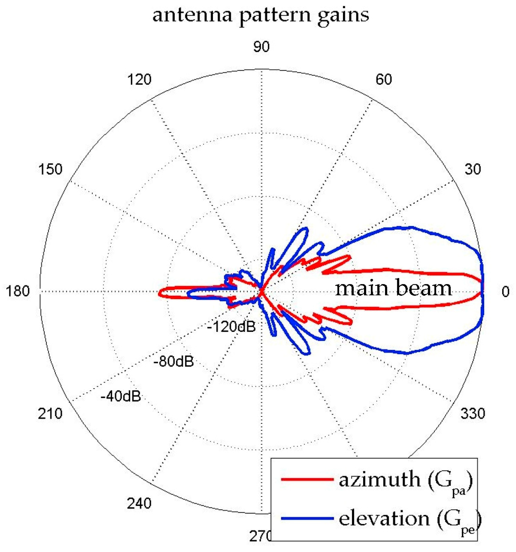
VV (vertical transmit and vertical receive) polarized K-MC3 transceiver module made by RFbeam Microwave GmbH in St. Gallen, Switzerland will be used, which transmits 24 GHz continuous wave with narrow beam widths, seven degrees in azimuth and 25 degrees in elevation, as shown in Figure 5. The seven-degree beam width in the azimuth enables the radar transceiver to transmit and receive in a specified direction; and the 25 degrees beam width in elevation includes not only the far facets but also the close ones at the sea surface.
Another important parameter in Equation (4) is the sea surface RCS ( σ ) . The microwave backscattering from the sea surface has been investigated by many researchers. One of the dominant scattering mechanisms at microwave frequencies and low-to-medium grazing angle is Bragg scattering, and non-Bragg scattering from the breaking waves was also observed and studied at a low-grazing angle [26,27,28,29]. According to the electromagnetic scattering perturbation theory, the first-order backscatter cross-sections were established in [30]. The radar cross-section for backscattering from capillary waves for VV and HH (horizontal transmit and horizontal receive) polarization and the results of measurements in the wind wave tank with an X-band radar was introduced in [31]. A mathematical model of normalized radar cross-section (NRCS) for Bragg backscattering and breaking wave in equilibrium conditions was presented in [32]. Microwave Doppler spectra models based on Bragg-scattering and composite-surface theory were developed and used to show backscattering from rough water surfaces under many wind speed and incidence angle conditions [33]. The backscattering mechanism from rough sea surface for both Ku- and C-bands was studied with the small-slope approximation method and a theoretical model for numerical calculations of a radar backscattering cross section was presented in [34].
The transceiver module has VV polarization so that the backscattering is dominated by Bragg scattering. Therefore, we use the mathematical model of NRCS for Bragg backscattering established under equilibrium condition [32]:
σ 0 = π β 0 2 2 | cos Φ | 1 2 sin 1 2 θ cot 1 4 θ F v v ( θ ) ( u 2 κ g ) 1 2 ,
where β 0 is the attenuation coefficient, Φ the direction of observation relative to wind, θ the incidence angle, u the friction velocity, κ the radar wavenumber, and F v v ( θ ) the first-order scattering coefficient for VV polarization [35]:
F v v ( θ ) = | ( ε r     1 ) [ ε r ( 1   +   sin 2 θ )     sin 2 θ ] [ ε r cos θ   +   ( ε r   sin 2 θ ) 1 / 2 ] 2 | 2 ,
where ε r is the relative complex dielectric constant of sea water. Although the NRCS model was established for equilibrium conditions, Phillips compared it with some radar experiments and concluded that it can be extended to a wide range of applications. Table 2 shows the parameters used for the NRCS calculation.
Here, ε r is the relative dielectric constant for sea water with salinity of 35 ppt and a temperature of 0 °C [36], u is a measured value with 7.3 m/s wind speed [
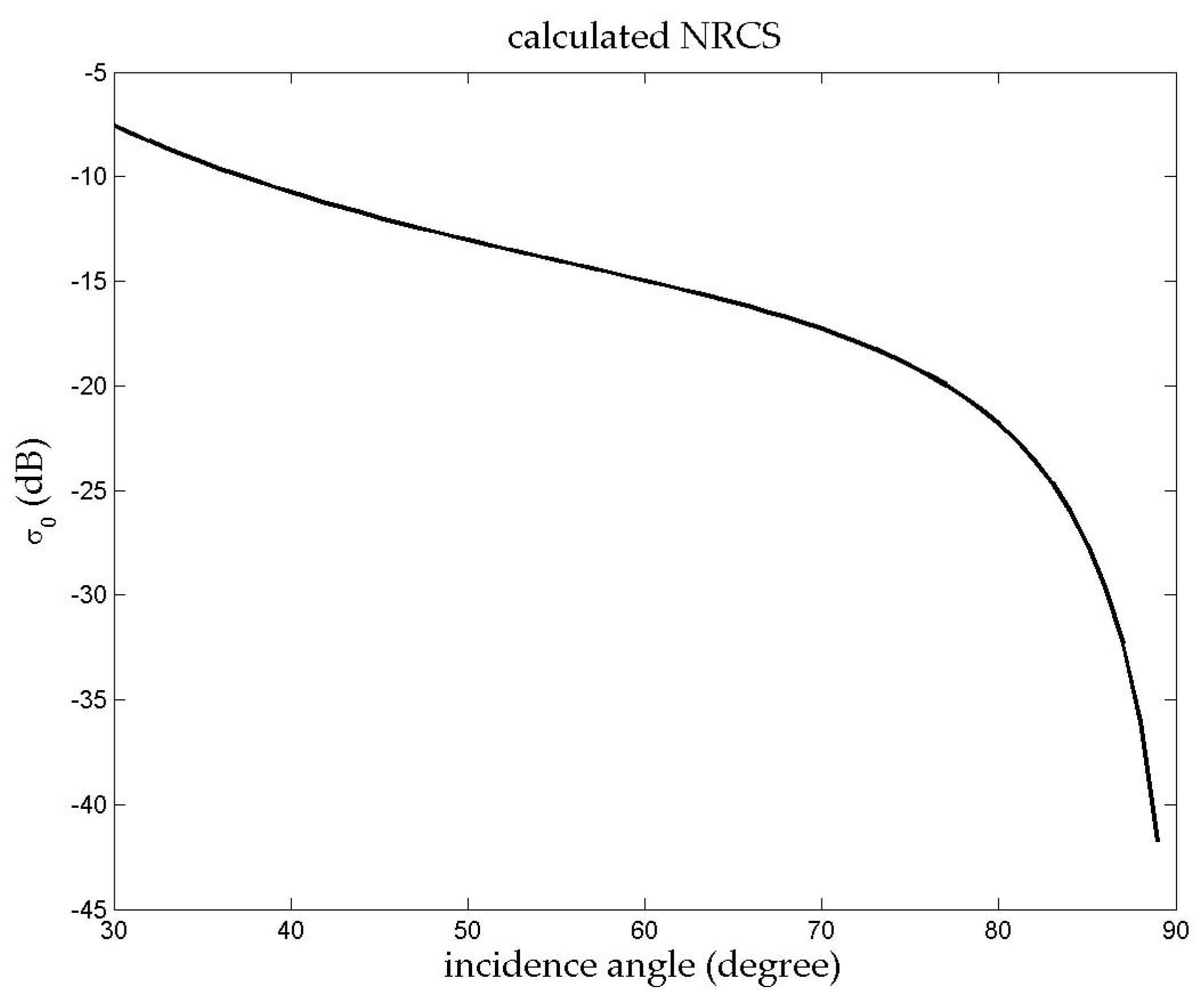
37]. The calculated NRCS is shown in Figure 6. The value at 90-degree is not shown in the figure because of much lower than others. The backscattering from the simulated sea surface is weak because the radar transceiver transmits and receives at a low-grazing angle, i.e., most of the incidence angles to the facets are approaching 90 degrees. Therefore, depressing the radar transceiver slightly is recommended to increase the radar grazing angle. Here the grazing angle is five degrees. Table 3 shows the parameters of numerical simulation conditions about ocean wave, wave field, radar transceiver, and IF signal.
For the given simulation conditions, the IF component power from each facet can be determined from Equation (4). The 
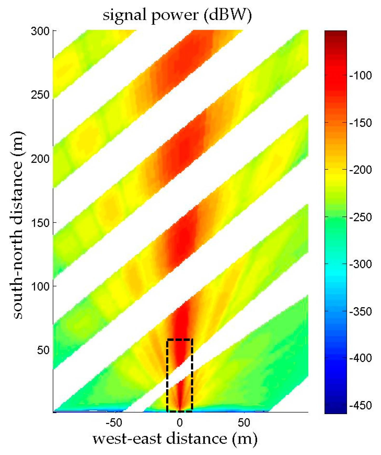
IF component power distribution, as shown in Figure 7, is obtained if the IF component powers are laid out on the wave field. The blank areas are the geometric shadows in which the facets cannot be seen by the radar transceiver. For microwave backscattering, partial shadowing [38] may cause some signals from the geometrically shadowed areas. However, they are invisible and below the noise floor because of low incident power. The warm color areas, which stand for the relatively strong scattering, are confined within the narrow azimuthal beam width of the radar transceiver.
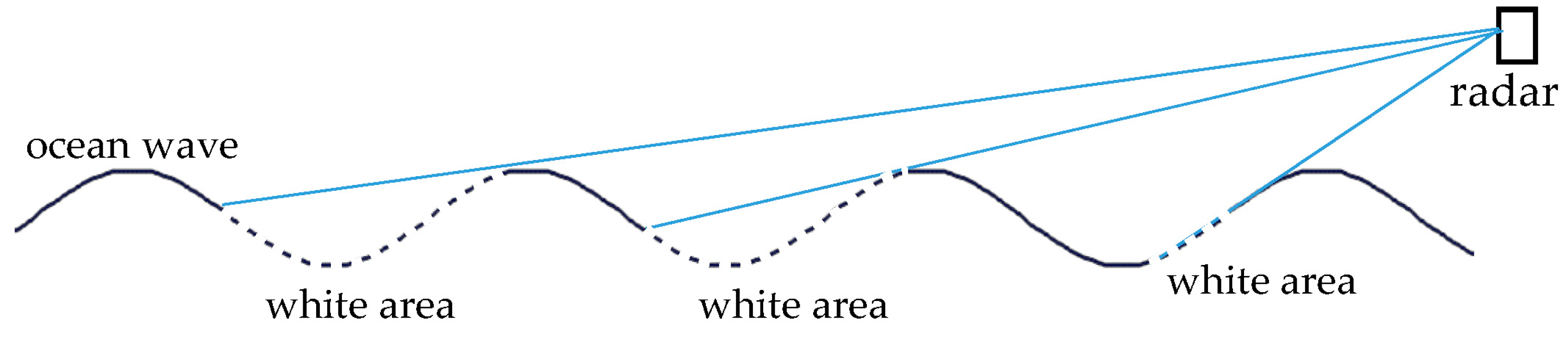
From the geometric viewpoint, the closer the wave approaches to the radar, the more surface of the wave the radar can see (see Figure 8). Thus, the white area at shorter range is narrower than those at longer ranges. Contrarily, the white areas are gradually getting wider at long range, as shown in 
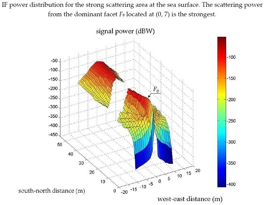
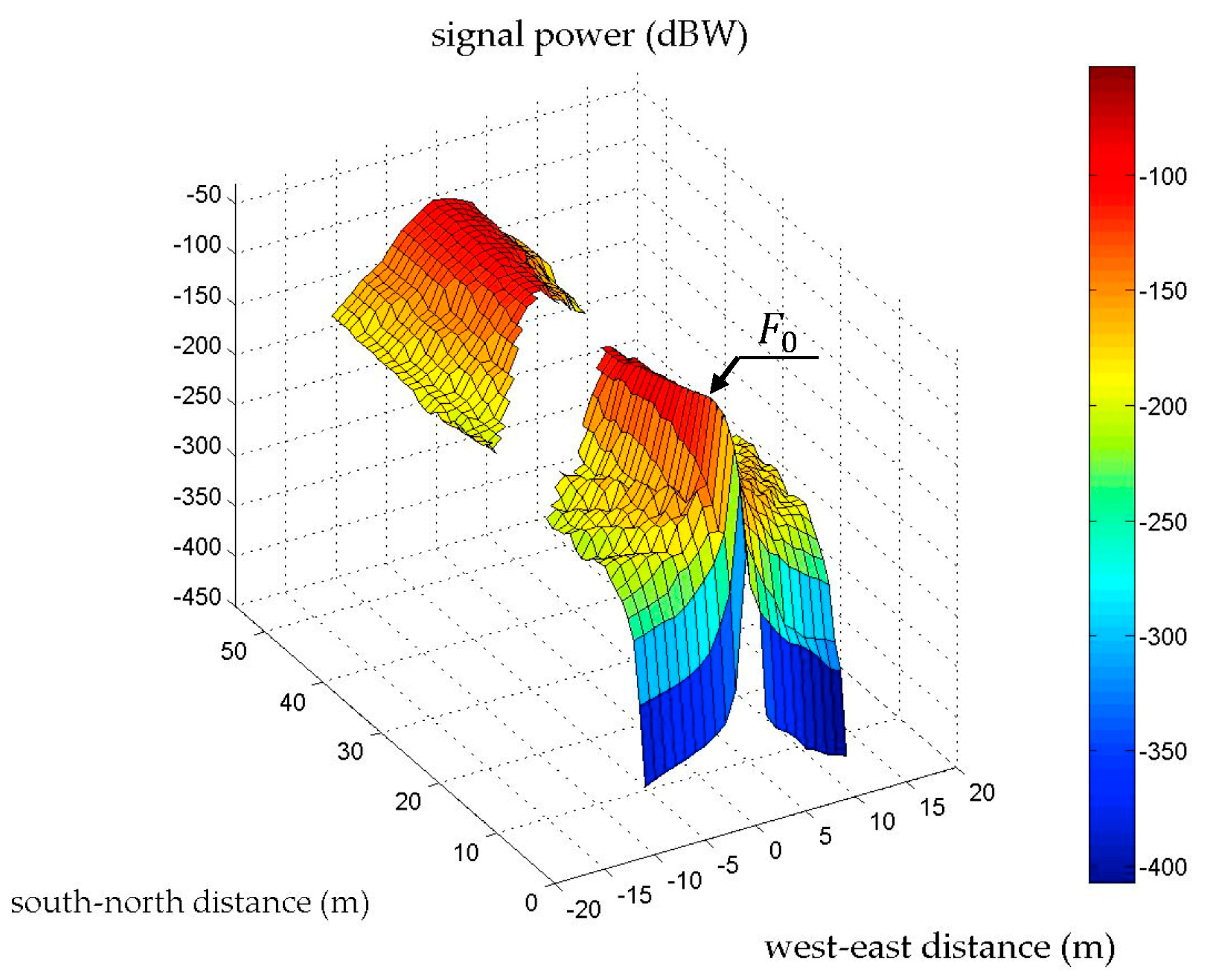
Figure 7. Strong scattering appears at locations close to the radar transceiver, and Figure 9 shows the 3-D plot of the IF power distribution of the strong scattering area which is marked as the dashed rectangle with a size of 55 m × 20 m in Figure 7. 
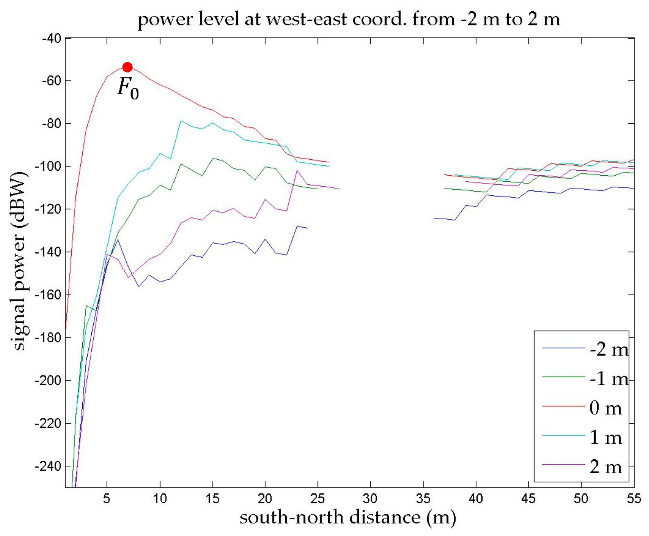
Figure 10 shows the powers distribution with the west-east coordinates from −2 m to 2 m. The power level at dominant facet the F 0 is much higher than for the side facets whose coordinates are −2 m, −1 m, 1 m, and 2 m.
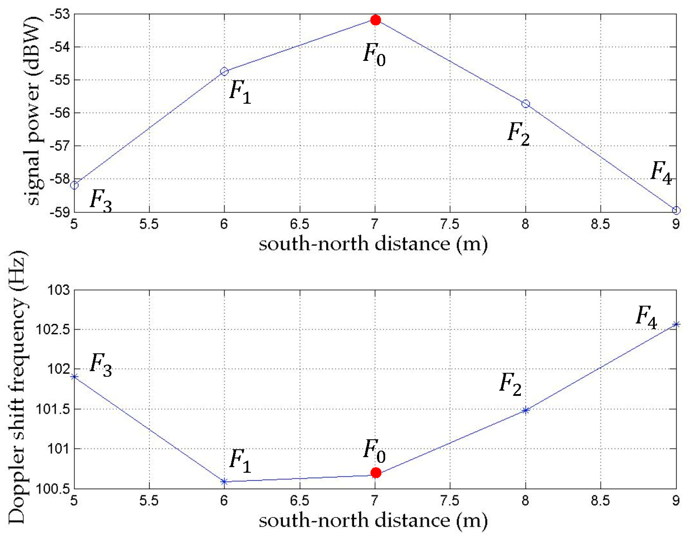
Figure 11 shows the power levels and Doppler shift frequencies of dominant facet F 0 and its four adjacent facets with the west-east coordinate being 0 m. The power of F 0 is not much higher than that of the two facets next to it, F 1 and F 2 , but the Doppler shift frequencies of these three facets are almost same. However, the power of F 0 is much higher than that of the two facets F 3 and F 4 .
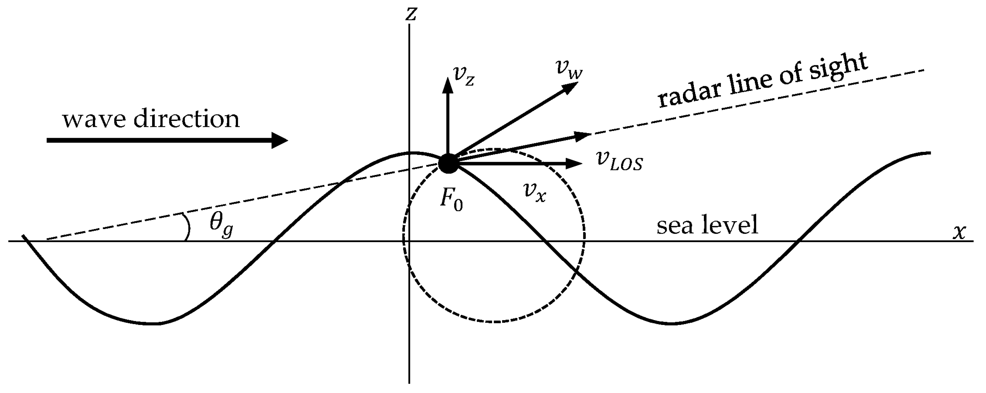
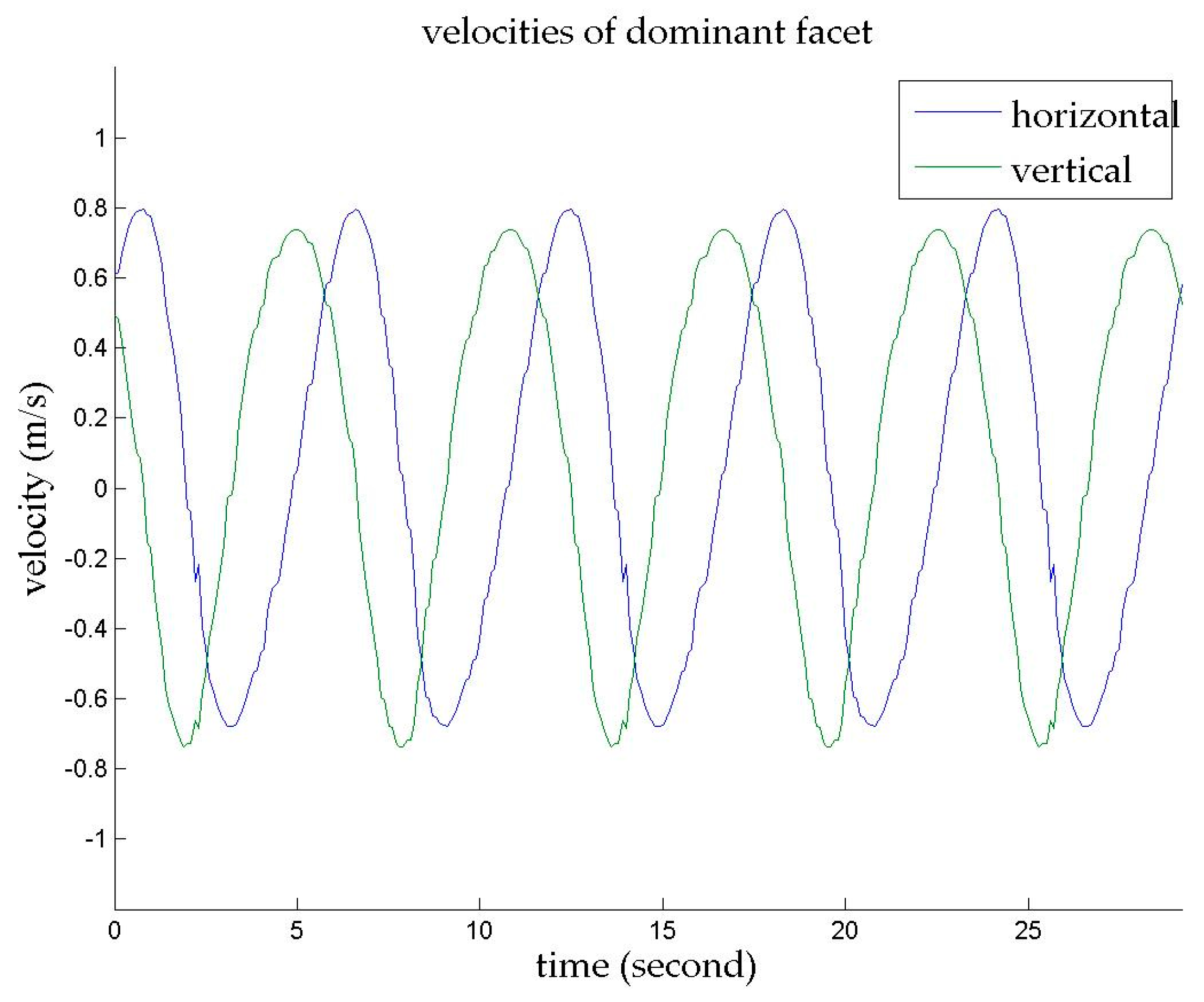
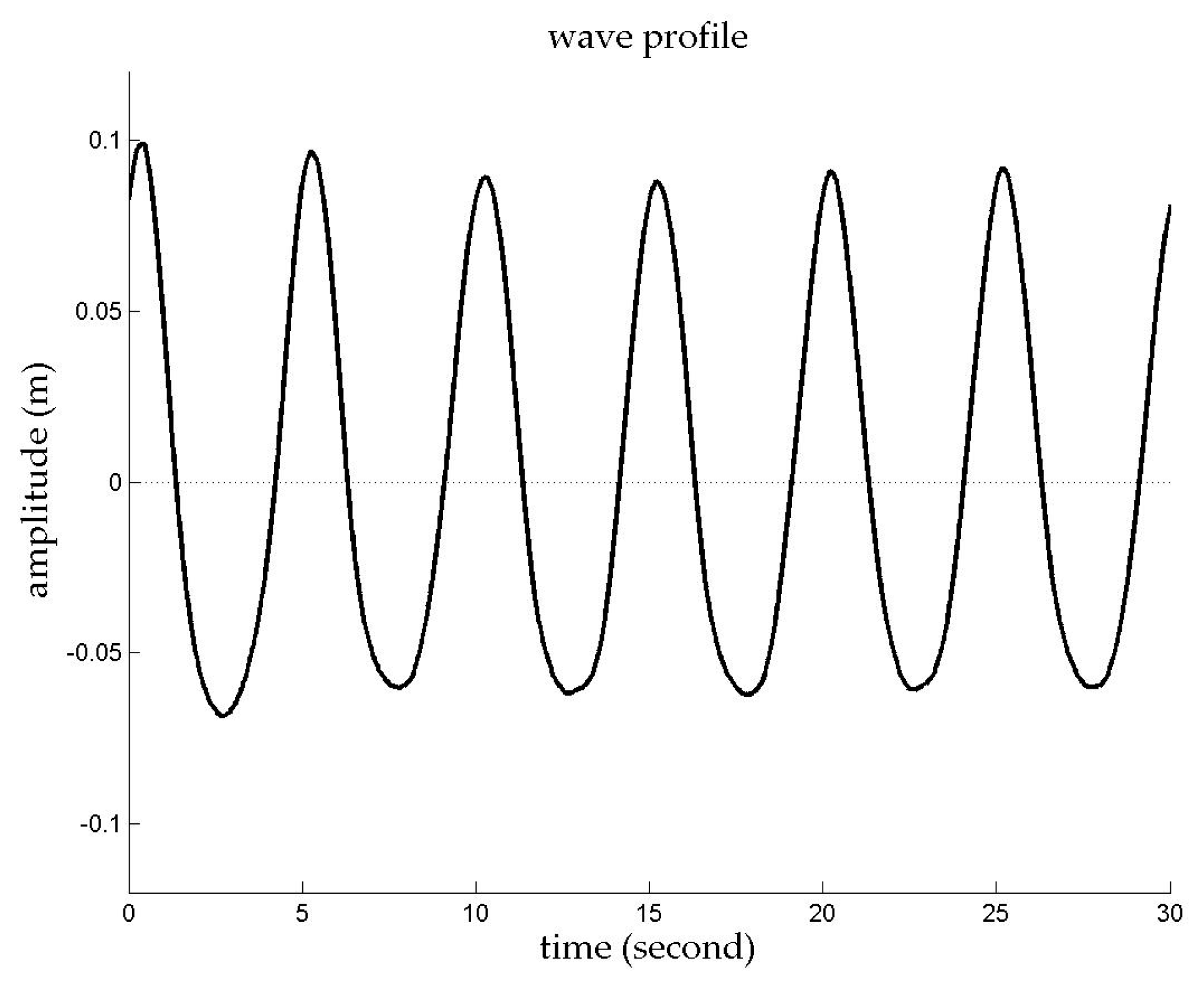
Figure 12 shows the horizontal velocity and vertical velocity of the dominant facet F 0 in five wave periods (29.25 s). The curves are sinusoids and oscillate with same amplitude, and the phase difference is π/2. Therefore, the motions of the dominant facet F 0 represent the orbital motions of the generated ocean waves.

3.3. Signal Processing and Results

The calculations of the power P I F , frequency f d , and phase φ of the IF component originated from each facet of the simulated ocean waves have been introduced. The total IF signal is the sum of the 
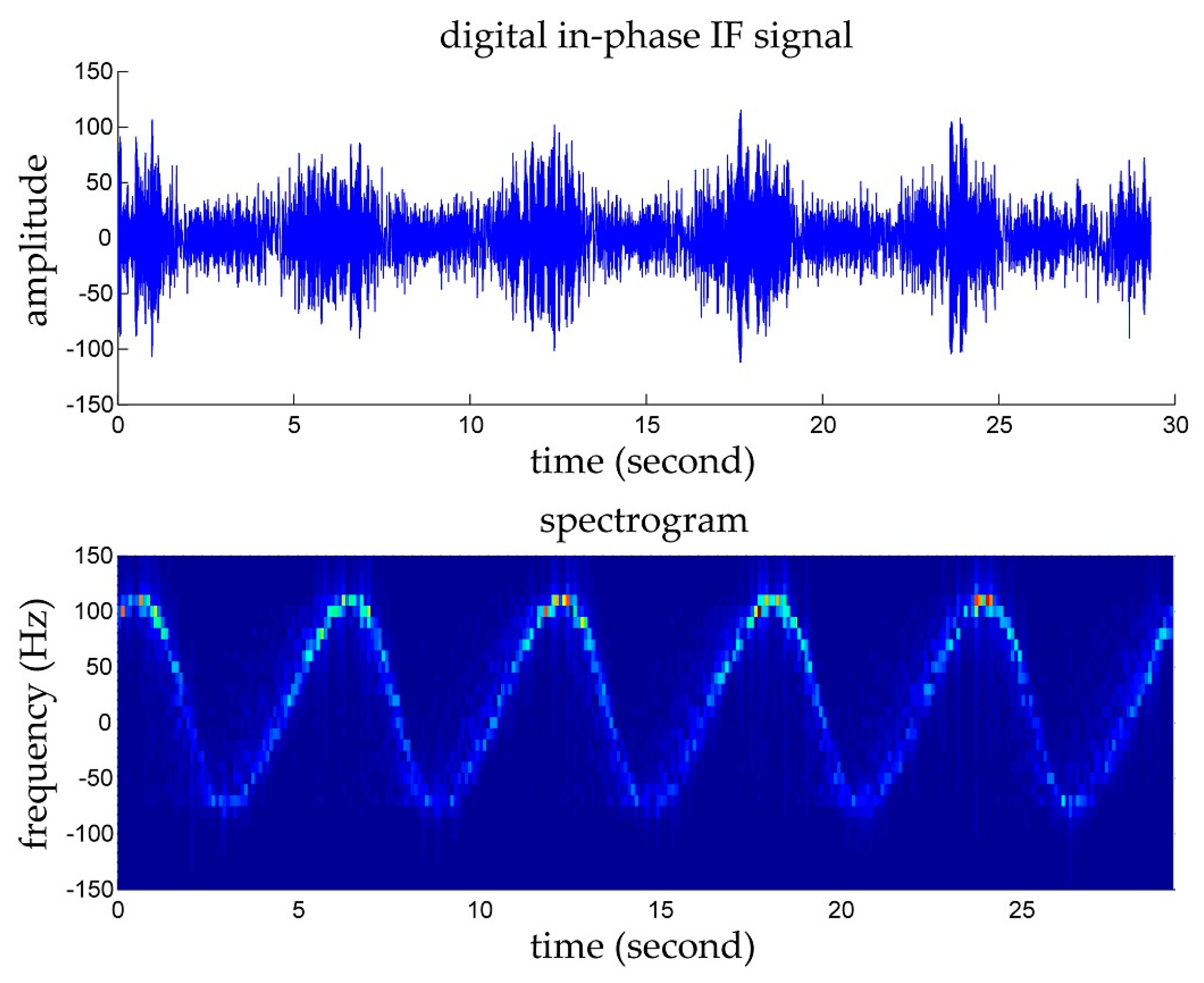
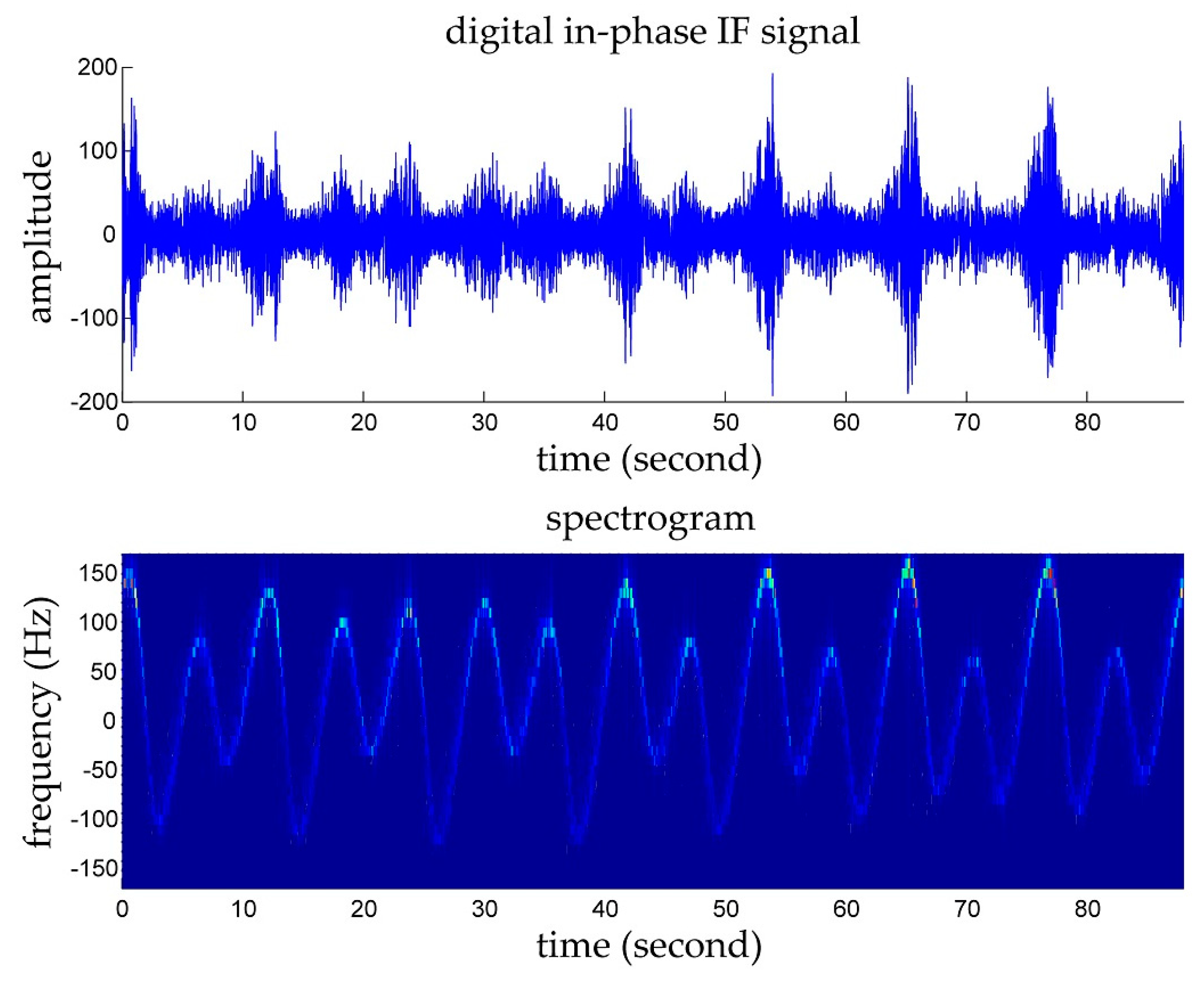
IF components and noise components. The IF signal and its spectrogram are shown in Figure 13. In the spectrogram, a bright line appears and is almost synchronized with the horizontal velocity of the dominant facet F 0 in Figure 12. This implies that the dominant facet F 0 dominates the received power from the simulated sea surface, and the bright line illustrates the variation of the Doppler shift frequency caused by the motions of the dominant facet F 0 . The bright line is extracted by finding the maximum value at each moment.
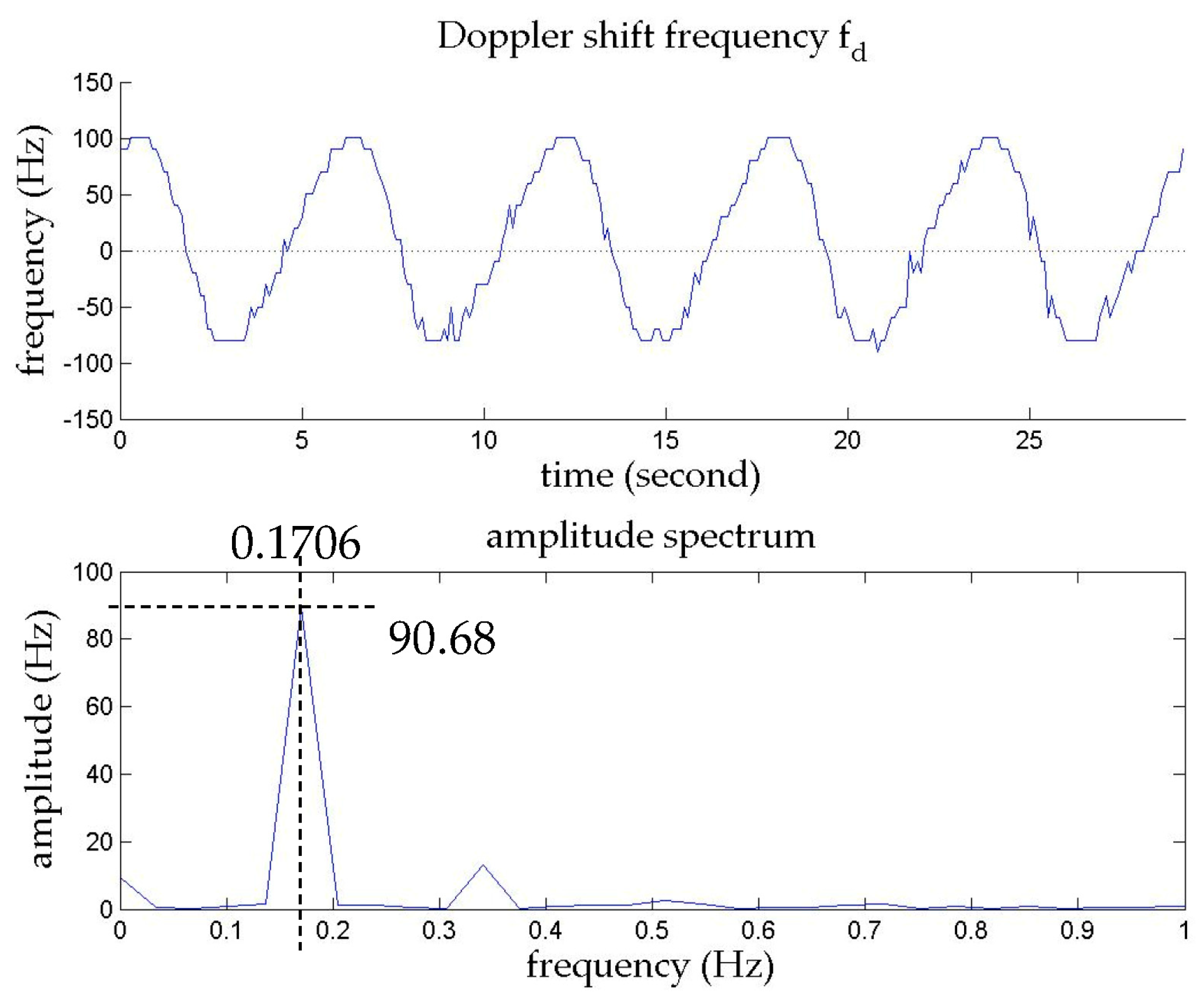
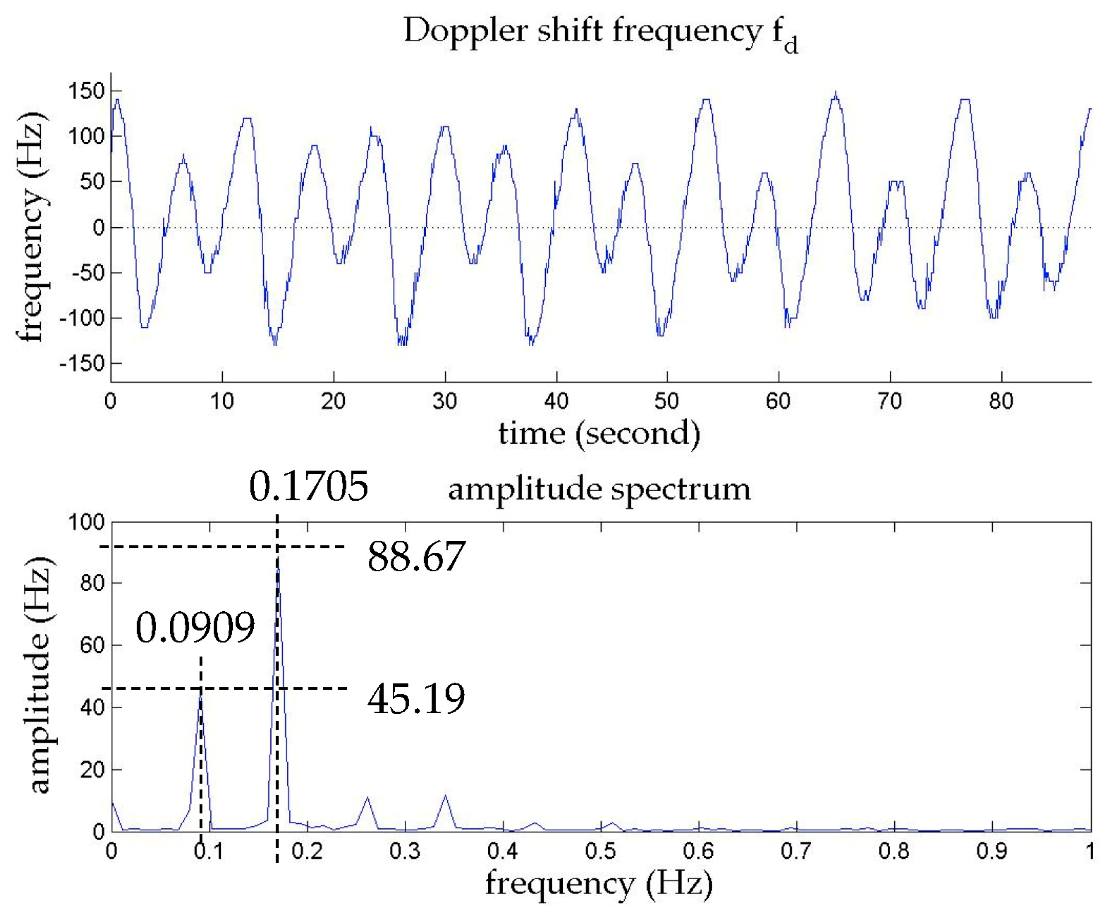
The extracted bright line, i.e., the time series of the Doppler shift frequency f d , and its amplitude spectrum are plotted in Figure 14. A significant peak can be seen in the amplitude spectrum and the corresponding amplitude and frequency are 90.68 Hz and 0.1706 Hz. Therefore, A d is 90.68 Hz and T d is 5.86 s. Substituting T d and A d into Equations (9) and (10), the measured wave period and wave height are 5.86 s and 1.05 m, respectively.
In addition to the significant peak at 0.1706 Hz, some other secondary peaks show up at the integer multiples of the frequency 0.1706 Hz because the velocities of the dominant facet are calculated according to Equations (5) and (6), which contain not only sinusoidal terms but also hyperbolic terms. According to the Taylor Series expansion of hyperbolic functions, the terms of cosh and sinh with variable z can be expressed as an infinite sum of terms which contain zn, n = 0, 1, 2, 3, …. Therefore the harmonics of the wave frequency exist in the velocities of the dominant facet as the result of the vertical coordinate z varying with same period of the generated wave.
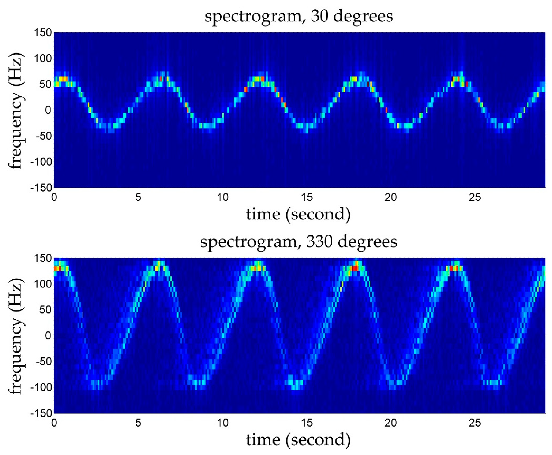
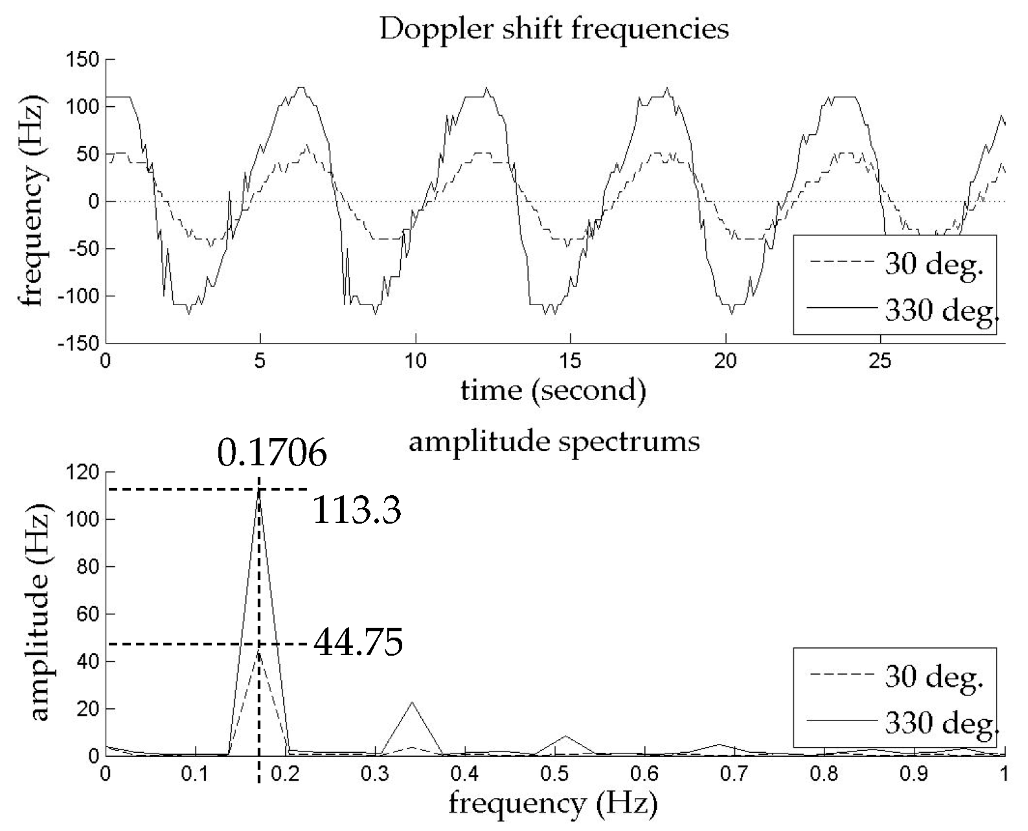
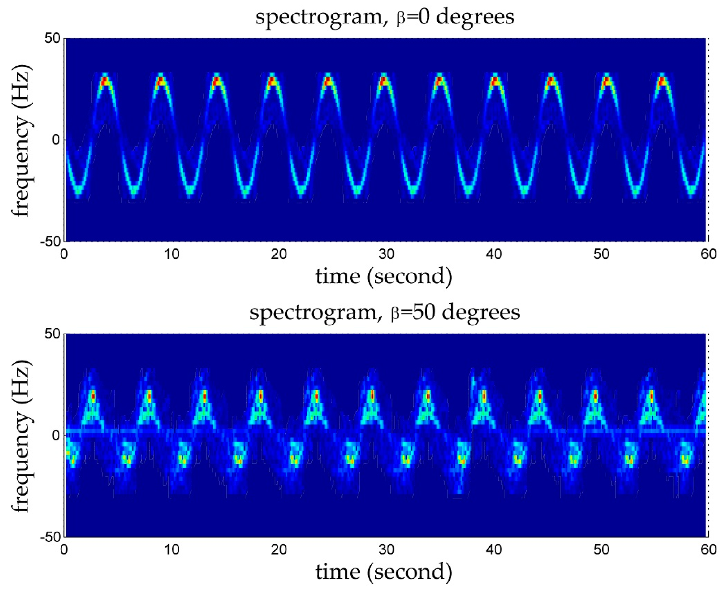
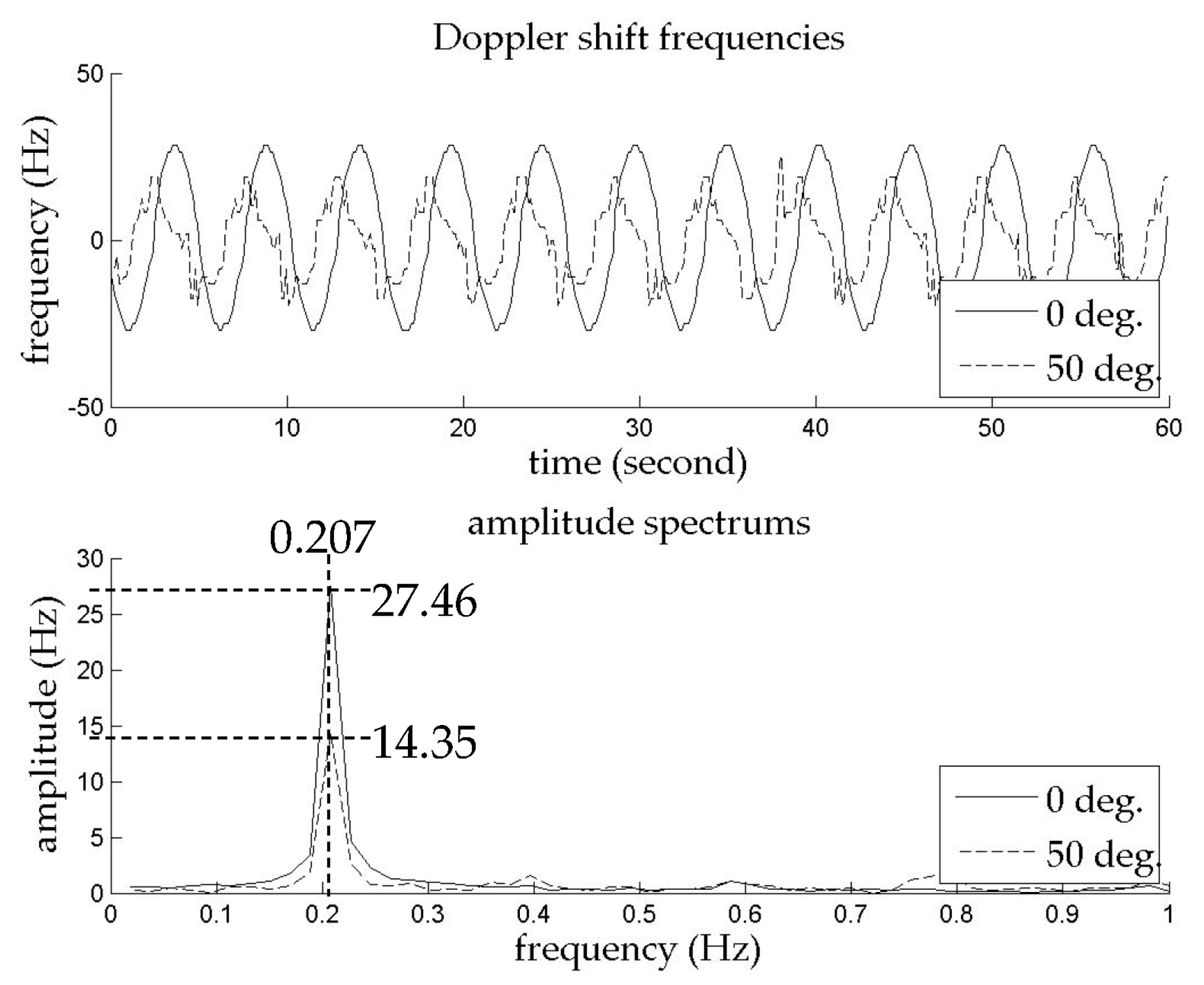
Two other simulations were executed for two radar directions, 30 degrees and 330 degrees. Two spectrograms of the IF signals are shown in Figure 15. Two extracted Doppler shift frequencies and two amplitude spectra are shown in Figure 16.
Similarly, two sets of results of wave period and height are obtained and shown in Table 4 with the first results. The three measured wave periods are identical, 5.84 Hz, which are very close to the period of the simulated ocean wave. The error mainly comes from the frequency resolution of the amplitude spectrum.
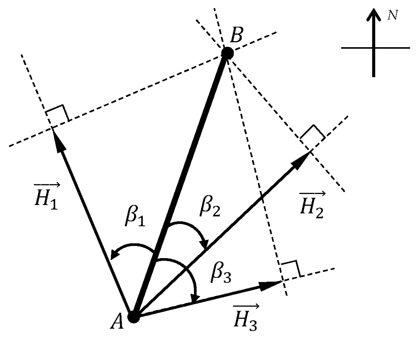
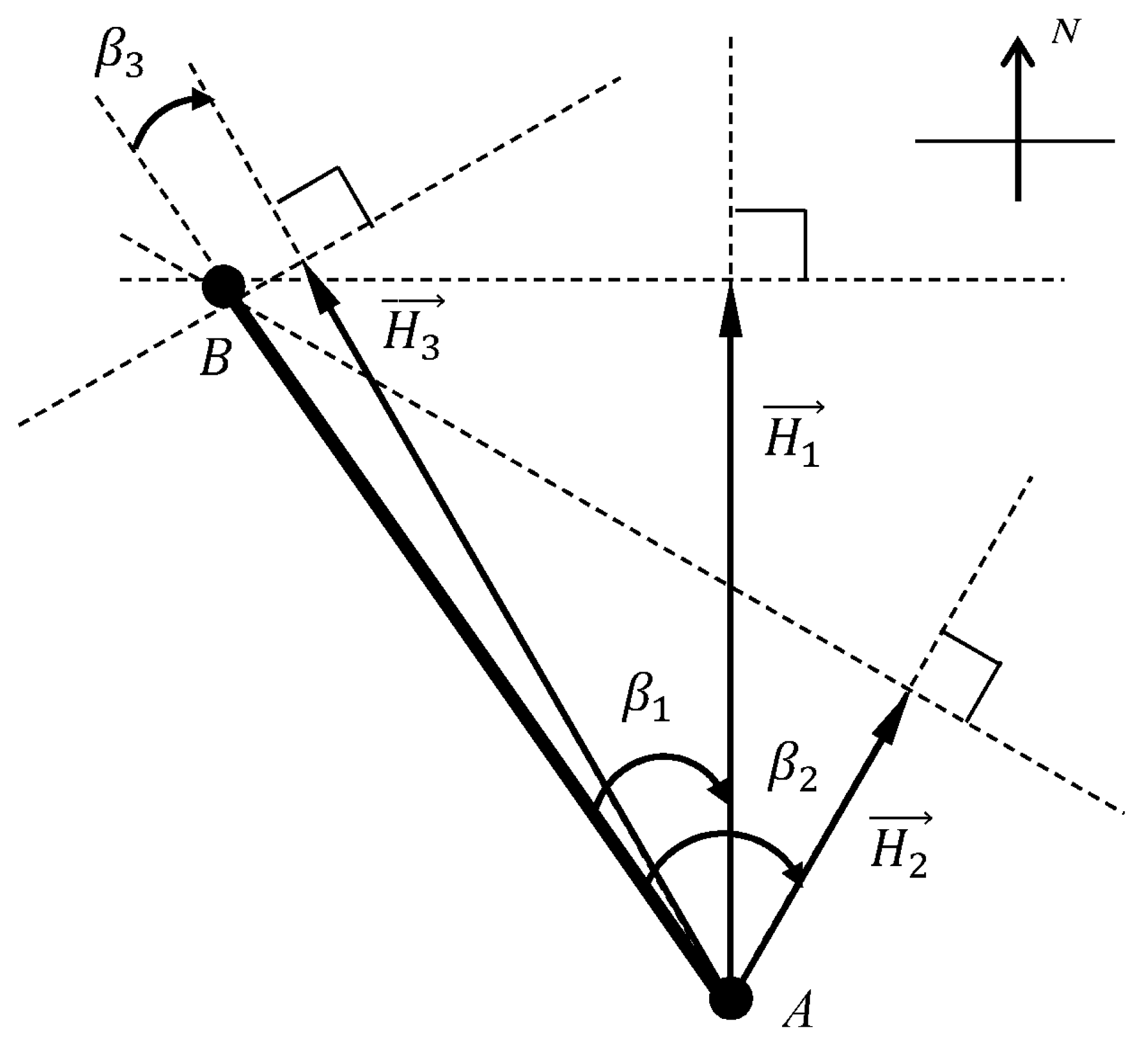
Three measured wave heights are less than 1.37 m because of the angles to the wave direction. Similarly, the true wave height can be retrieved with three measured wave heights and three radar directions, as shown in Figure 17.
In this case, these perpendicular lines cannot cross because of the wave height measurement errors. Here, the centroid B of the intersecting points of the perpendiculars is used. The length of the line segment AB, 1.33 m, is the final result of wave height measurement and the wave direction is measured to be about 142.13 degrees. The resultant measurement approximates the wave height and direction in the simulation conditions but with errors of 3.7% and 1.5%, respectively. There are three main error sources: the frequency resolution in the spectrogram of IF signal; the noise components in IF signal; the constructive or destructive scattering originated from the facets adjacent to the dominant facet F 0 . The errors can be greatly decreased if the frequency resolution and the extraction method are improved.

3.4. Measurement of Multiple Ocean Waves

Considering the ocean waves generated by a distant storm and propagating into the wave field shown in Figure 4, two ocean waves present and the respective characteristics are shown in Table 5. The wave 1 is identical with the previous simulations. The period of wave 2 is 10.97 s which is consistent with the period T p generated by 15 m/s wind, but the wave height has reduced to 1 m. Wave 1 and wave 2 are superposed in the wave field (see Figure 18). Figure 19 includes the in-phase IF signal and the spectrogram of the IF signal in fifteen periods of wave 1 (87.75 s).
The bright line in the spectrogram demonstrates the fluctuations of the Doppler shift frequency, and it obviously contains multiple frequency components. Figure 20 shows the extracted Doppler shift frequency and its amplitude spectrum. Two significant peaks stand out indicating the amplitudes and frequencies for the two waves.
Table 6 shows the simulation results as well as some wave characteristics. The wave heights are calculated with Equation (10) and amended with the angles to wave. The measured wave periods and the amended wave heights are very close to the settings shown in Table 5. Furthermore, the true values of the wave heights can be obtained by measuring in several different directions when the wave directions and the angles to wave are unknown.

4. Validation in the Wave Tank

4.1. Experimental Configurations

The validation experiment was conducted in the wave tank of the Fluids Laboratory of Memorial University of Newfoundland. The tank is 50 m long and 4.5 m wide, and 1.8 m deep. The short-range K-band NBCWR was mounted on the towing carriage about 2 m above the water surface. Figure 21 shows the radar installation in the wave tank. Additionally, two wave sensors were also used to profile the generated waves. The experimental configurations are shown in Table 7. The wave period and height were set by the wave generator of the wave tank. The wavelength was measured with the two wave sensors. Figure 22 shows the wave profiles output of one of the wave sensors. It can be seen that six waves passed in 30 s because of the 5-s wave period, and the troughs are wider than the crests because the troughs were slowed down by the friction from the bottom of the tank.

4.2. Experimental Results

The short-range K-band NBCWR measured the generated waves in two angles to wave, 0 degrees and 50 degrees, respectively. Two 60-s spectrograms of the IF signals for two measurement directions are shown in Figure 23. By comparing the two spectrograms, the strong signals which denote the Doppler shift frequencies caused by the dominant facets at the surface are fluctuating in almost the same period but different amplitudes. The extracted Doppler shift frequencies and the amplitude spectrums are shown in Figure 24. Two significant peaks show up in the amplitude spectrums to manifest the periods and amplitudes of the variations of the Doppler shift frequencies. The Doppler frequency variation range depends on | cos ( β ) | . It drops significantly for the case of β = 50-deg since the coefficient cos(50°) is smaller than cos(0).
The measurement results are shown in Table 8 and the bottom row gives the wave height obtained with the geometrical relationship of the two results, H 1 and H 2 . The measured period (4.81 s) and height (0.1552 m) are very close to the configured values of the generated wave, and errors are less than 3.8% and 3.5%, respectively. The measurement accuracy could be improved if more signals were sampled and more directions were applied.

5. Discussion

We performed the numerical simulation and validated the existence of the dominant facet, as shown in Figure 10 and Figure 11. Given space limitations, we cannot present more cases with different simulation conditions. However, the waves were successfully measured in the simulation for multiple waves and the experiment in wave tank. It implies that dominant facets existed and oscillated with wave propagations. The dominant facet just has a size of a few square meters and is very close to the radar. Therefore, the technique provides a possibility of measuring ocean waves by sensing a small facet in a limited local area but not scanning a large area of sea surface to generate a radar image. The technique can be applied to surface craft and offshore platform to measure local ocean waves for enhancing operation safety.
In order to improve measurement accuracy, the size of dominant facet must be formed as small as possible because the orbital velocities of the points on a small dominant facet are much more uniform than those on a large one. The facet size can be reduced by using radar transceiver with a much narrower beam and setting the radar transceiver much closer to the sea surface. For this reason, the technique cannot be applied if the sensor is installed at a relatively high location, in which case a large dominant facet is formed, but inconsistent orbital velocities exist.
In the numerical simulations and the wave tank experiment, we also found that there were always errors in the measured heights, periods, and directions. There are three main error sources: the frequency resolution in the spectrogram of IF signal; the noise components in IF signal; and the constructive or destructive scattering originated from the facets adjacent to the dominant facet. As shown in Figure 17, the true wave height measurement has error because of the errors of three wave height measurements. This also causes wave direction measurement errors as well as a 180-degree ambiguity. However, the errors can be greatly decreased if the frequency resolution and the extraction method are improved. The frequency resolution can be improved by extending the total sampling time because the frequency resolution of amplitude spectrum is equal to the reciprocal of total sampling time. With a higher frequency resolution, we can select the significant peaks at the frequencies much closer to the true wave frequencies. In additions, the extracted time series of Doppler shift frequency have some noise components which might introduce errors even if the regular waves are used in numerical simulations and tank experiments. The error may be reduced by considering the weighted average of the values around the maximum value at a certain moment on bright line. Improved method and a study of the effect of sampling time on measurement error at complex sea sate will be investigated in the future.
Meanwhile, we considered only the wave propagations which contributed the periodical components of Doppler shift frequency. In practice, the phase velocity of Bragg scattering wave, velocity of the surface current, and wind-induced surface drift usually add non-periodical components to the Doppler shift frequency. However, these non-periodical components can be identified and removed in the phase of data processing. In addition, platform motions cause additional components which can be identified by recording the platform’s relative velocity to the average position of the dominate facet. These operations cannot completely remove undesired components but the remainders are weak and negligible.
Regular waves were used in the numerical simulations and the wave tank experiments. Therefore, the orbital motions of the regular waves can be explained by linear wave theory, and the wave periods and heights were calculated using Equations (9) and (10), which are based on linear wave theory. The impacts of wind and wave age are not included. The simulated waves had the same period and height as the spectral peak wave in the Pierson-Moskowitz spectrum; the waves in the tank were generated by the back-and-forth motions of the wave generator but not by wind. However wind waves at the real sea surface are not regular waves. The horizontal and vertical components of the dominant facet’s velocities caused by wind waves can be explained more precisely using nonlinear wave theory. According to the Stokes’ second-order theory, the horizontal and vertical components are functions of wave period, height, and steepness [39]. Wind wave steepness is a function of wave age and young age wind waves are much steeper, as described in [40], and a wind-wave spectrum model described in [41] shows how wave age affects the spectral peak and energy distribution, which is also used to retrieve the wind speed [42]. Consequently, if wind waves show up in an amplitude spectrum, the wave age must be taken into consideration to improve the accuracy of the retrieval of wave period and height.
The amplitude spectrum measured at the real sea surface can be transformed to the wave spectrum in a specific direction. If many wave spectra for different directions are obtained, directional wave spectra can be established, which presents the wave energy distribution in the wave frequency and direction. The range of wave spectrum measurements is limited. It depends on the relative size of the dominant facet to the wave lengths. A capillary wave cannot be measured if its whole waveform is totally covered by the dominant facet, and a long period gravity wave cannot be measured if the component of Doppler shift frequency caused by it is less than the frequency resolution in the spectrogram of the IF signal.

6. Conclusions

In this paper, a measurement method of period, height and direction of ocean wave is presented. The short-range K-band NBCWR is employed as the wave sensor to measure orbital motions of ocean waves at low-grazing angle. The measurement is not based on the image generated by scanning sea surface but based on a dominant facet at the sea surface.
In the numerical simulations, we used the dominant waves from the Pierson-Moskowitz spectrum, the typical antenna pattern gains of the K-MC3 transceiver module and the K-band NRCS for Bragg backscattering. IF power distribution illustrates the existence of the dominant facet. It can be identified that it oscillates with wave propagations and its motions represent the orbital motions of the ocean waves. Wave period and height were obtained through measuring the period and amplitude of the variation of Doppler shift frequency caused by the dominant facet, and wave direction was deduced with the geometrical relationship of the measurement results in different directions. The multiple waves were measured as well.
In the wave tank validation experiments, we configured the radar with the same conditions as those for the numerical simulations. The generated wave is measured in two angles to the wave, 0 degrees and 50 degrees, respectively. The IF signals were strong enough to allow us to distinguish the Doppler shift frequencies and the strong signal in spectrograms shows the existence of the dominant facet. The measurement results were consistent with the characteristics of the generated wave. Therefore, the proposed method is reasonable and potentially feasible for ocean wave measurement.

Author Contributions

J.C. performed the numerical simulations and experiments and drafted the manuscript. R.B., B.d.Y., and W.H. supervised the study, and contributed to the design of the experiments and the interpretation of the results. All the authors contributed to the editing of the manuscript.

Funding

This research was undertaken as part of the Ice Ocean Sentinel System (IOSS) project, funded by the Canadian Atlantic Innovation Fund (#781-2636-201155) the Research and Development Corporation Newfoundland, the Province of Newfoundland and the Terra Nova Project.

Acknowledgments

The research is part of the research of the unmanned surface craft program funded by Ice Ocean Sentinel System, Atlantic Innovation Funds. The authors appreciate the assistance and support of Neil Riggs, Haibing Wang, and Federico Luchino during the development of the short-range K-band NBCWR and the wave tank experiments.

Conflicts of Interest

The authors declare no conflict of interest.

Abbreviations

The following abbreviations are used in this manuscript:
HHHorizontal transmit and Horizontal receive
IFIntermediate Frequency
LOSLine Of Sight
NBCWRNarrow Beam Continuous Wave Radar
NRCSNormalized Radar Cross Section
RCSRadar Cross Section
VVVertical transmit and Vertical receive

References

  1. Thomson, E.R.; Emery, J.W. Data Analysis Methods in Physical Oceanography, 3rd ed.; Newnes: Oxford, UK, 2014; pp. 77–78. ISBN 978-0-12-387782-6. [Google Scholar]
  2. Chen, A.C.; Nihoul, C.J.J. Oceanography—Volume III; EOLSS Publications: Oxford, UK, 2009; pp. 116–118. ISBN 978-1-905839-64-3. [Google Scholar]
  3. Wyatt, L.R. High-frequency radar measurements of the ocean wave-directional spectrum. IEEE J. Ocean. Eng. 1991, 16, 163–169. [Google Scholar] [CrossRef]
  4. Barrick, D.E. The ocean wave height non-directional spectrum from inversion of the HF sea-echo Doppler spectrum. Remote Sens. Environ. 1977, 201–227. [Google Scholar] [CrossRef]
  5. Huang, W.; Wu, S.; Gill, E.; Wen, B. HF radar wave and wind measurement over the eastern China Sea. IEEE Trans. Geosci. Remote Sens. 2002, 40, 1950–1955. [Google Scholar] [CrossRef]
  6. Zhao, C.; Chen, Z.; Jiang, Y.; Fan, L.; Zhen, G. Exploration and validation of wave-height measurement using multifrequency HF radar. Am. Meteorol. Soc. 2013, 30, 2189–2202. [Google Scholar] [CrossRef]
  7. Trizna, B.D. Coherent marine radar measurements of ocean surface currents and directional wave spectra. In Proceedings of the OCEANS 2011 IEEE—Spain, Santander, Spain, 6–9 June 2011. [Google Scholar] [CrossRef]
  8. Borge, J.; Hessner, K.; Reichert, K. Estimation of the significant wave height with X-band nautical radars. In Proceedings of the 28th International Conference on Offshore Mechanics and Arctic Engineering (OMAE), St. John’s, NL, Canada, 11–16 July 1999. [Google Scholar]
  9. Carrasco, B.; Horstmann, J.; Seemann, J. Significant wave height measured by coherent X-band radar. IEEE Trans. Geosci. Remote Sens. 2017, 55, 5355–5365. [Google Scholar] [CrossRef]
  10. Wang, H.; Li, H.; Zhang, Y.; Guo, L. The measurement of sea surface profile with X-band coherent marine radar. Acta Oceanol. Sin. 2015, 34, 65–70. [Google Scholar] [CrossRef]
  11. Trizna, B.D. Method and Apparatus for Coherent Marine Radar Measurements of Properties of Ocean Waves and Currents. U.S. Patent US8305257 B2, 6 November 2012. [Google Scholar]
  12. Seemann, J.; Senet, M.C.; Ziemer, F. Method for Determining Hydrographic Parameters Which Describe a Sea Swell Field In Situ Using a Radar Device. U.S. Patent US6775617 B2, 10 August 2004. [Google Scholar]
  13. Marom, M.; Goldstein, R.M.; Thornton, E.B.; Shemer, L. Remote sensing of ocean wave spectra by interferometric synthetic aperture radar. Nature 1990, 345, 793–795. [Google Scholar] [CrossRef]
  14. Goldstein, R.M.; Barnett, T.P.; Zebker, H.A. Remote sensing of ocean currents. Science 1989, 246, 1282–1285. [Google Scholar] [CrossRef] [PubMed]
  15. Schuler, D.L.; Keller, W.C. Pier-based Measurements of Ocean Wave Spectra Using Three-frequency Ku- and L-band Radars. In Proceedings of the 12th Canadian Symposium on Remote Sensing Geoscience and Remote Sensing Symposium, Vancouver, BC, Canada, 10–14 July 1989. [Google Scholar] [CrossRef]
  16. Cui, J.; Bachmayer, R.; deYoung, B.; Huang, W. Retrieval of ocean wave characteristics from K-band radar. In Proceedings of the OCEANS 2016 MTS/IEEE, Monterey, CA, USA, 19–23 September 2016. [Google Scholar] [CrossRef]
  17. Gray, J.O.; Caldwell, G.D. Advanced Robotics & Intelligent Machines; IET: Stevenage, UK, 1996; pp. 165–168. ISBN 978-0852968536. [Google Scholar]
  18. Raju, G.S.N. Radar Engineering; I. K. International Pvt Ltd.: New Delhi, India, 2008; pp. 55–56. ISBN 13 978-8190694216. [Google Scholar]
  19. Silver, S. Microwave Antenna Theory and Design; IET, Technology & Engineering: Stevenage, UK, 1949; pp. 2–6. ISBN 0-86341-017-0. [Google Scholar]
  20. Sorensen, M.R. Basic Wave Mechanics: For. Coastal and Ocean. Engineers; John Wiley & Sons: New York, NY, USA, 1993; pp. 14–17. ISBN 978-0471551652. [Google Scholar]
  21. Lewandowski, M.E. The Dynamics of Marine Craft: Maneuvering and Seakeeping, Volume 22 of Advanced Series on Ocean. Engineering; World Scientific: London, UK, 2004; pp. 146–147. ISBN 978-9810247560. [Google Scholar]
  22. Sawaragi, T. Coastal Engineering—Waves, Beaches, Wave-Structure Interactions, Volume 78 of Developments in Geotechnical Engineering; Elsevier: Amsterdam, The Netherlands, 1995; pp. 7–11. ISBN 978-0-444-82068-6. [Google Scholar]
  23. Dixon, R. Radio Receiver Design; CRC Press: Boca Raton, FL, USA, 1998; pp. 79–100. ISBN 0-8247-0161-5. [Google Scholar]
  24. Zhang, Z.; Moore, C.J. Mathematical and Physical Fundamentals of Climate Change; Elsevier: Amsterdam, The Netherlands, 2014; pp. 433–434. ISBN 978-0-12-800066-3. [Google Scholar]
  25. Türke, U. Efficient Methods for WCDMA Radio Network Planning and Optimization; Springer Science & Business Media: New York, NY, USA, 2007; pp. 36–38. ISBN 978-3-8350-5456-1. [Google Scholar]
  26. Haykin, S. Remote Sensing of Sea Ice and Icebergs; John Wiley & Sons: New York, NY, USA, 1994; p. 474. ISBN 978-0-471-55494-3. [Google Scholar]
  27. Werle, B.O. Sea backscatter, spikes and wave group observations at low grazing angles. In Proceedings of the IEEE Radar Conference, Alexandria, VA, USA, 8–11 May 1995. [Google Scholar] [CrossRef]
  28. Twarog, E.M.; McLaughlin, D.J.; Allan, N. High resolution polarimetric radar scattering measurements of low grazing angle sea clutter. In Proceedings of the IEEE Geoscience and Remote Sensing Symposium, Lincoln, NE, USA, 31 May 1996. [Google Scholar] [CrossRef]
  29. Lee, P.H.Y.; Barter, J.D.; Caponi, E.; Caponi, M.; Hindman, C.L.; Lake, B.M.; Rungaldier, H. Wind-speed dependence of small-grazing-angle microwave backscatter from sea surfaces. IEEE Trans. Antennas Propag. 1996, 44, 333–340. [Google Scholar] [CrossRef]
  30. Peake, W.H. Theory of radar return from terrain. In Proceedings of the 1958 IRE National Convention Record, New York, NY, USA, 21–25 March 1966. [Google Scholar] [CrossRef]
  31. Wright, W.J. Backscattering from capillary waves with application to sea clutter. IEEE Trans. Antennas Propag. 1966, 14, 749–754. [Google Scholar] [CrossRef]
  32. Phillips, O. Radar return from the sea surface—Bragg scattering and breaking waves. J. Phys. Oceanogr. 1998, 18, 1065–1074. [Google Scholar] [CrossRef]
  33. Plant, W.J.; Keller, C.W. Evidence of Bragg scattering in microwave Doppler spectra of sea return. J. Geophys. Res. 1990, 95, 16299–16310. [Google Scholar] [CrossRef]
  34. Voronovich, A.G.; Zavorotny, V.U. Theoretical model for scattering of radar signals in Ku- and C-bands from a rough sea surface with breaking waves. Waves Random Media 2001, 11, 247–269. [Google Scholar] [CrossRef]
  35. Valenzuela, R.G. Theories for the interaction of electromagnetic and oceanic waves—A review. Bound.-Layer Meteorol. 1978, 13, 61–85. [Google Scholar] [CrossRef]
  36. Meissner, T.; Wentz, J.F. The complex dielectric constant of pure and sea water from microwave satellite observations. IEEE Trans. Geosci. Remote Sens. 2004, 42, 1836–1849. [Google Scholar] [CrossRef] [Green Version]
  37. Vickers, D.; Mahrt, L.; Andreas, LF.E. Formulation of the sea surface friction velocity in terms of the mean wind and bulk stability. J. Appl. Meteorol. Climtol. 2015, 54, 691–703. [Google Scholar] [CrossRef]
  38. Plant, J.W.; Farquharson, G. Wave shadowing and modulation of microwave backscatter from the ocean. J. Geophys. Res. 2012, 117, C08010. [Google Scholar] [CrossRef]
  39. McCormick, M.E. Ocean. Engineering Mechanics: With Applications; Cambridge University Press: Cambridge, UK, 2010; pp. 86–87. ISBN 0521859522. [Google Scholar]
  40. Liu, B.; Ding, Y.; Guan, C.L. A relationship between wave steepness and wave age for wind waves in deep water. Chin. J. Oceanol. Limol. 2007, 25, 36–41. [Google Scholar] [CrossRef]
  41. Cheng, Y.; Liu, Y.; Xu, Q. A new wind-wave spectrum model for deep water. Indian J. Geo-Mar. Sci. 2006, 35, 181–194. [Google Scholar]
  42. Cheng, Y.; Xu, Q.; Liu, Y.; Lin, H.; Xiu, P.; Yin, X.; Zong, H.; Rong, Z. An analytical algorithm with a wave age factor for altimeter wind speed retrieval. Int. J. Remote Sens. 2008, 29, 5699–5716. [Google Scholar] [CrossRef]
Figure 1. Relationships between wave orbital velocity, ocean wave characteristics, and Doppler shift frequency. The wave measurement starts from measuring Doppler shift frequency with the radar. The variation of the measured Doppler shift frequency contains the information of the wave period, height, and direction. It is explained with the relationship   γ 3 , which is deduced from γ 1 and γ 2 .
Remotesensing 10 01242 g001
Figure 2. Velocities of the dominant facet F 0 orbiting with a long surface wave. The radar is not shown here, but it transmits from right to left along the LOS and it is close to the sea surface. v x , v z and v L O S are three projections of v w to x-axis, z-axis, and LOS, respectively. Compared with v x , the phase of v L O S is delayed by θ g .
Remotesensing 10 01242 g002
Figure 3. Geometrical relationship between the true wave height and three measured wave heights. All the directions are measured with respect to north.
Remotesensing 10 01242 g003
Figure 4. Top view of regular wave field, T = 5.85 s and L = 53.35 m. The radar’s location is (0, 0) and it transmits to the north. Wave direction is 140 degrees, measured clockwise from the north.
Remotesensing 10 01242 g004
Figure 5. Antenna pattern of the K-MC3 transceiver module. The antenna’s 3 dB beam widths in azimuth and elevation are seven degrees and 25 degrees, respectively.
Remotesensing 10 01242 g005
Figure 6. NRCS σ 0 for a VV polarized antenna (upwind). This is a calculated NRCS for a K-band radar under certain wind and sea water conditions as shown in Table 2.
Remotesensing 10 01242 g006
Figure 7. IF component power distribution. The strongest power −53 dBW occurs at the dominant facet which is located at (0, 7) in the main lobe. Some directional spreading around the main lobe also presents because of the side lobes as shown in Figure 5, but all of them are over 100 dBW under the power from dominant facet so that they have hardly any impact on the measurement.
Remotesensing 10 01242 g007
Figure 8. Size variation of white area. The solid parts of the curve are visible to the radar but the dashed parts are invisible.
Remotesensing 10 01242 g008
Figure 9. IF power distribution for the strong scattering area. The scattering power from the dominant facet located at (0, 7) is the strongest.
Remotesensing 10 01242 g009
Figure 10. Power comparison around the dominant facet F 0 . The absence of middle parts of the curves is due to the shadowed facets. The power levels at the dominant facet are much higher than the other four curves. Therefore, the scattering from side facets are negligible in the radar IF output.
Remotesensing 10 01242 g010
Figure 11. Comparison of Doppler shift frequency and signal power for dominant facet F 0 and four adjacent facets. The power level of the adjacent facets decline rapidly so that the received power at the radar is dominated by the facet F 0 .
Remotesensing 10 01242 g011
Figure 12. Horizontal velocity and vertical velocity of the dominant facet F 0 . The velocities are calculated according to Equations (5) and (6), in which the variation of spatial position (x, z) of the dominant facet is also taken into account.
Remotesensing 10 01242 g012
Figure 13. IF signal and its spectrogram. The upper figure is the in-phase signal and the fluctuation of its amplitude reflects the wave propagation. The quadrature signal is not shown here. The in-phase signal and quadrature signal are the real part and the imaginary part of the complex IF signal, respectively. The strong signal in the lower figure originates from the dominant facet F 0 .
Remotesensing 10 01242 g013
Figure 14. Extracted Doppler shift frequency and its amplitude spectrum. A harmonic of wave frequency can be found at the frequency 0.3412 Hz.
Remotesensing 10 01242 g014
Figure 15. Spectrograms for two radar looking directions. Compared with the spectrogram in Figure 13, the Doppler shift frequency fluctuates with lower amplitude in the upper figure but higher amplitude in the lower figure. This is due to the coefficient | cos ( β ) | . The wave direction is 140 degrees, and the radar looking directions are 0, 30, and 130 degrees. Therefore, the angles to wave: β 1 = 40 degrees, β 2 = 70 degrees,   β 3 = 10 degrees and the coefficients: | cos ( β 1 ) | = 0.766,   | cos ( β 2 ) | = 0.342, | cos ( β 3 ) | = 0.980.
Remotesensing 10 01242 g015
Figure 16. Two extracted Doppler shift frequencies and amplitude spectrums. The harmonics of wave frequency exist.
Remotesensing 10 01242 g016
Figure 17. True wave height retrieval with three measured wave heights. The angles to wave: β 1 = 40 degrees, β 2 = 70 degrees, and   β 3 = 10 degrees.
Remotesensing 10 01242 g017
Figure 18. Two ocean waves. The highest points and the lowest points are 1.185 m and −1.185 m and located in the dark red areas and the dark blue areas, respectively.
Remotesensing 10 01242 g018
Figure 19. IF signal and its spectrogram for multiple ocean waves. In the lower figure, the Doppler shift frequency fluctuates with two frequencies corresponding to two wave frequencies 0.1709 Hz and 0.0912 Hz.
Remotesensing 10 01242 g019
Figure 20. Extracted Doppler shift frequency and its amplitude spectrum. The harmonics of the wave frequency exist.
Remotesensing 10 01242 g020
Figure 21. Experimental set-up in wave tank. The radar is fixed on the stationary blue carriage. The radar transceiver is the white square in the center of the red circle. It can rotate to transmit in different directions to adjust the angle to wave, β .
Remotesensing 10 01242 g021
Figure 22. Wave profile in the wave tank. The horizontal straight line at 0 m is assumed to be still water level. The values on the curve are the water surface elevations measured by wave sensor. Average wave height is 0.15 m; wave period is 5 s; wave length is 16.79 m which is measured with two separate wave sensors mounted along the propagation direction of the wave.
Remotesensing 10 01242 g022
Figure 23. Spectrograms for two measurement directions. The upper figure is the spectrogram which is obtained by pointing the radar transceiver to the wave coming direction, i.e., β = 0 degree; the lower figure is obtained by rotating the radar transceiver counter-clockwise 50 degrees from the wave coming direction, i.e., β   = 50 degrees.
Remotesensing 10 01242 g023
Figure 24. Two extracted Doppler shift frequencies and amplitude spectra. The angles to wave are 0 degrees and 50 degrees, and the coefficients: | cos ( 0 ) | = 1,   | cos ( 50 o ) | = 0.643.
Remotesensing 10 01242 g024
Table 1. Characteristics of waves at the spectral peak.
U (m/s)810121518
H s (m)1.3712.1433.0864.8216.943
f p (Hz)0.1710.1370.1140.0910.076
T p (s)5.8497.3118.77310.96613.159
L p (m)53.35083.359120.038187.559270.085
Table 2. NRCS calculation conditions.
ParametersValueUnit
β 0 0.01-
Φ 0 (upwind)degree
θ 30~90degree
ε r 16–32i-
u 0.22m/s
κ 2 π / 0.0125 rad/m
Sea water temperature0°C
Sea water salinity35ppt
Table 3. Numerical simulation conditions.
ParametersValuesUnit
Ocean wavePeriod ( T )5.85s
Height ( H )1.37m
Length ( L ) 53.35m
Water depth (d)1000m
Direction ( α )140degree
Wave fieldWidth200m
Length300m
NRCS ( σ 0 )Figure 6m2
Facet size1 × 1m2
TransceiverFrequency ( f T )24GHz
Position(0, 0)m
Height2m
Direction0 (north)degree
Grazing angle ( θ g )5degree
Output impedance ( R I F )100Ω
Output power ( P T )0.079W
Antenna gain ( G a n )21dBi
Amplifiers gain ( G a m )60dB
Pattern gains ( G p a , G p e )Figure 5dB
IF signalDuration29.25s
Noise voltage−93dBV/Hz
Sampling frequency10,240Hz
Precision12bit
Table 4. Three simulation results.
No.123Unit
Radar direction030330degree
Amplitude ( A d )90.6844.75113.3Hz
Wave period ( T )5.865.845.84s
Wave height ( H )1.05 ( H 1 )0.52 ( H 2 )1.32 ( H 3 )m
Angle to wave ( β )40 ( β 1 )70 ( β 2 )10 ( β 3 )degree
Table 5. Characteristics of two ocean waves.
CharacteristicsWave 1Wave 2Unit
period ( T )5.8510.97s
height ( H )1.371.00m
length ( L ) 53.35187.70m
Wave direction ( α )140180degree
Water depth (d)1000m
Table 6. Simulation results for two waves.
No.Wave 1Wave 2Unit
Wave direction ( α )140180degree
Amplitude ( A d )88.6745.19Hz
Wave period ( T )5.8711.00s
Wave height ( H )1.040.99m
Angle to wave ( β )400degree
Amended wave height1.360.99m
Table 7. Validation experiment configurations.
ParametersValuesUnit
WavePeriod ( T )5s
Average height ( H )0.15m
Length ( L ) 16.79m
Water depth (d)1.8m
TransceiverFrequency ( f T )24GHz
Height2m
Angle to wave ( β )0 and 50degree
Grazing angle ( θ g )5degree
IF signalDuration60s
Sampling frequency4375Hz
Table 8. Wave tank measurement results.
No.12Unit
Angle to wave ( β )050degree
Amplitude ( A d )27.4614.35Hz
Wave period ( T )4.814.81s
Wave height ( H )0.1534 ( H 1 )0.0807 ( H 2 )m
True wave height0.1552m

