Improving Data Quality for the Australian High Frequency Ocean Radar Network through Real-Time and Delayed-Mode Quality-Control Procedures


Abstract

1. Introduction
2. Materials and Methods
3. Results
3.1. Velocity Threshold Optimization
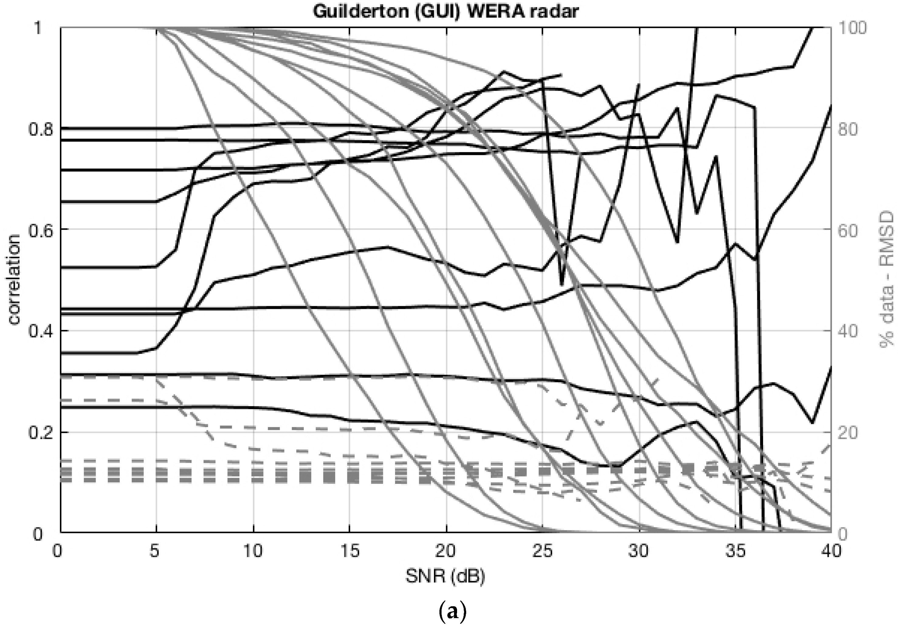
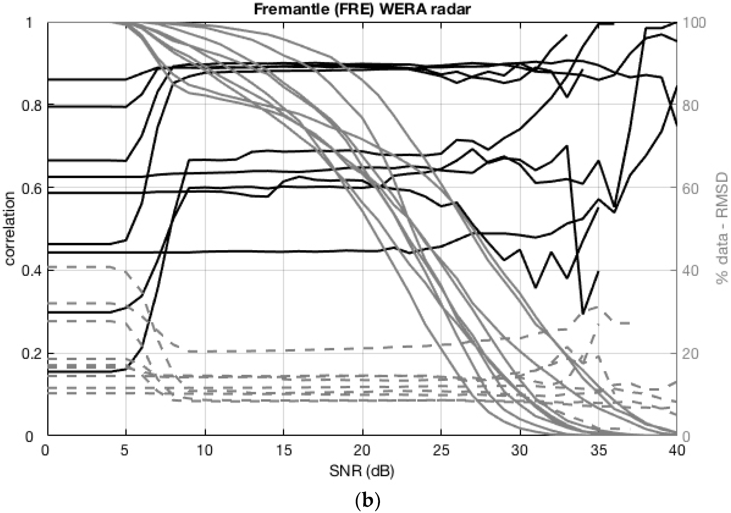
3.2. SNR Threshold Optimization
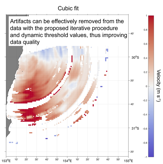
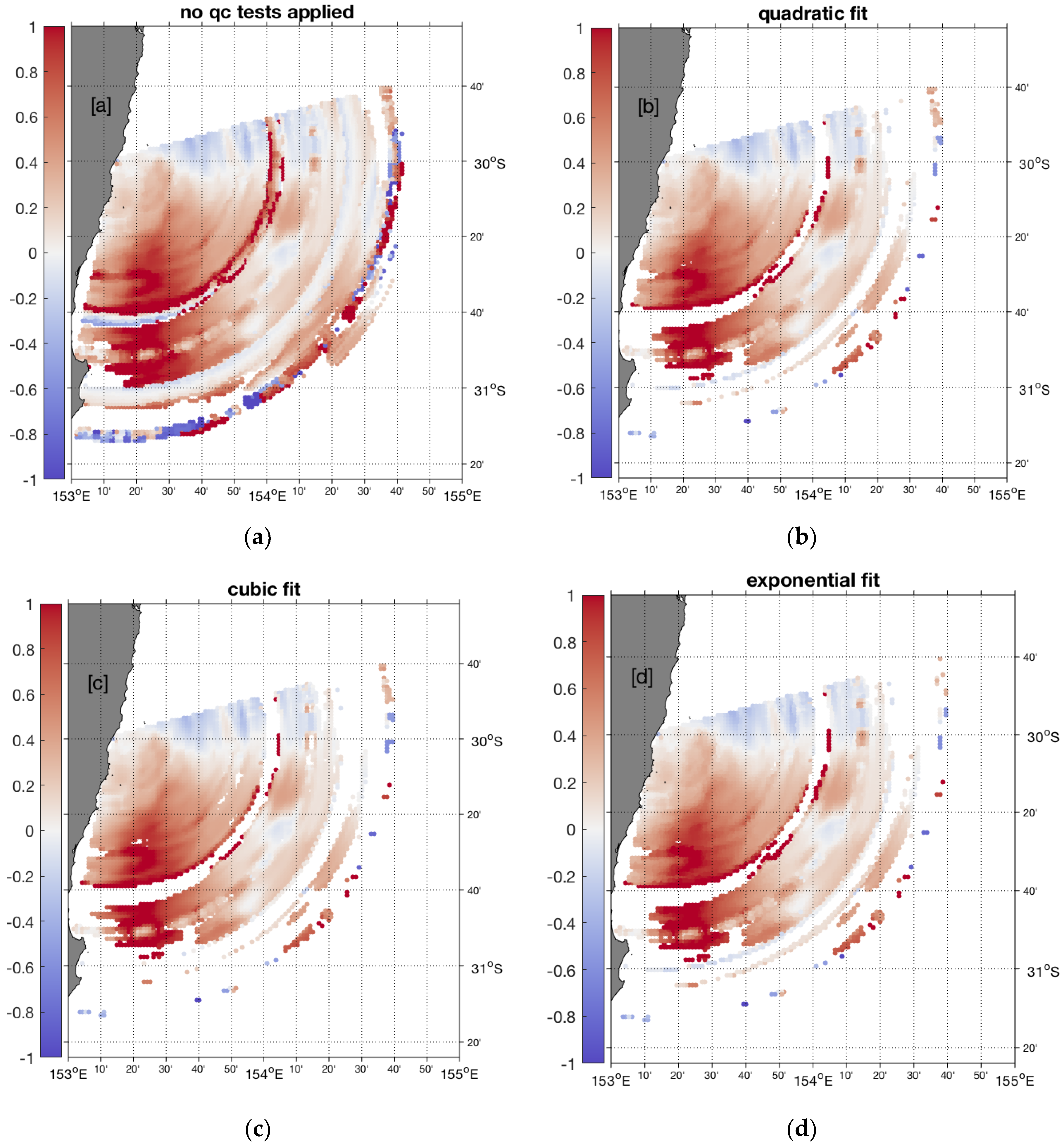
3.3. Advanced Artifact Removal
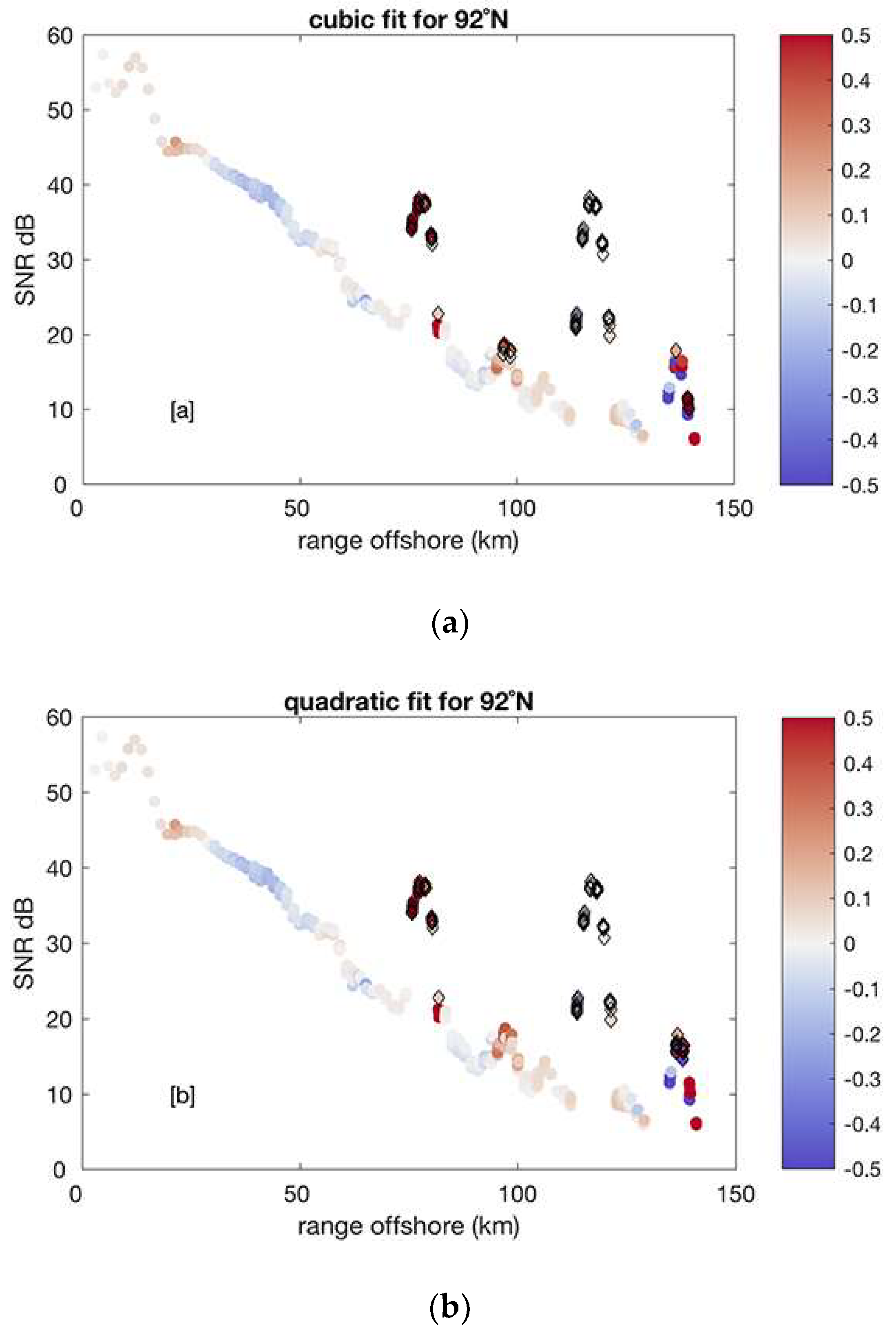
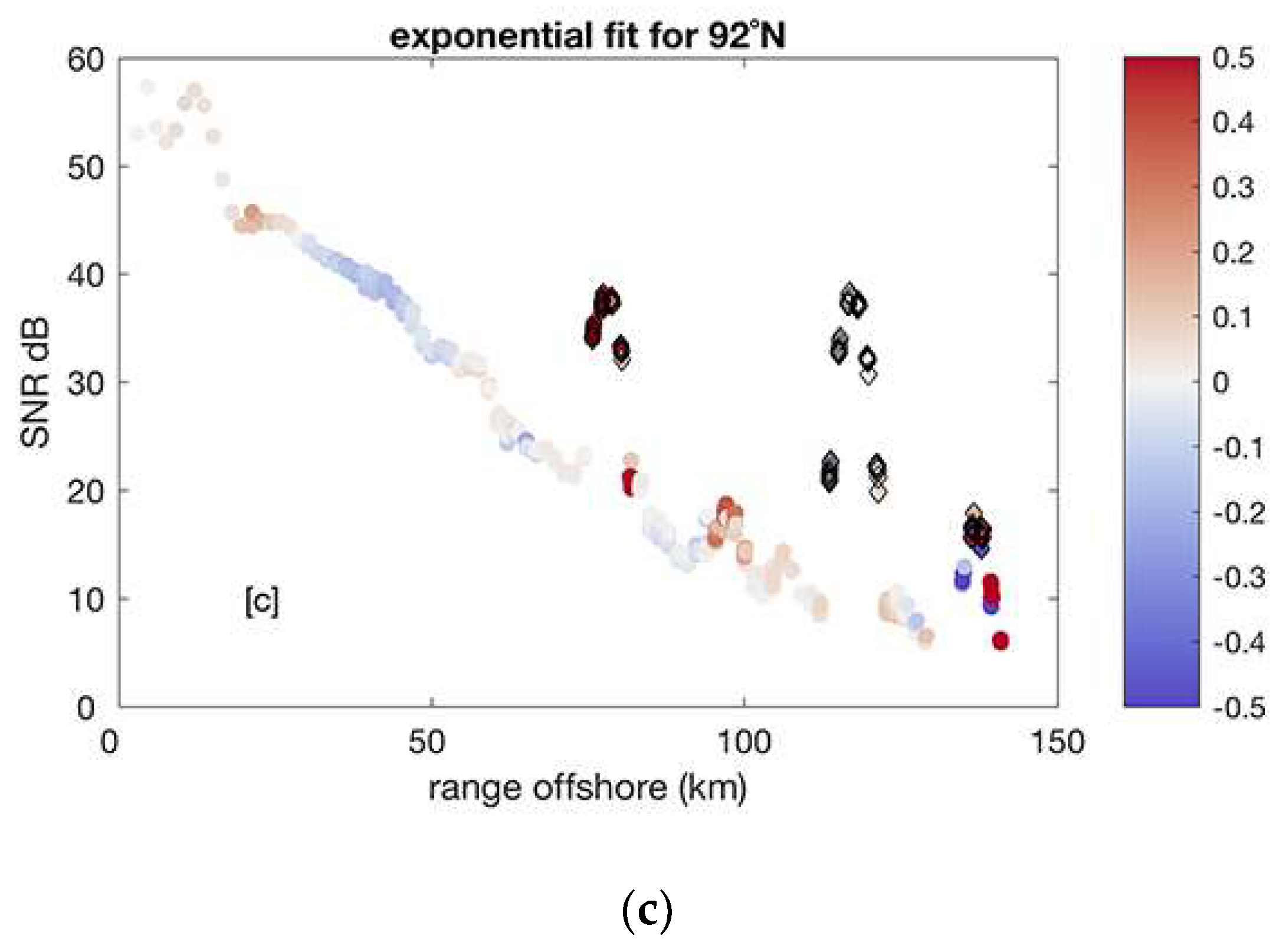
- fit a polynomial model to the SNR distribution along each radar beam (1-D case) or fit a 2-D surface to the SNR map;
- estimate a “distance” between the data and the polynomial fit and set confidence levels as n * σ(data-fit), where n = 2, 3;
- remove suspect SNR data outside of the confidence levels;
- move to the next radial beam (1-D case);
- repeat Steps 1–4 until (i) no more anomalous data are detected or (ii) a maximum number of iterations is reached.
4. Discussion
5. Conclusions
Author Contributions
Funding
Acknowledgments
Conflicts of Interest
References
- Archer, M.R.; Keating, S.R.; Roughan, M.; Johns, W.E.; Lumpkin, R.; Beron-Vera, F.; Shay, L.K. The kinematic similarity of two western boundary currents revealed by sustained high-resolution observations. Geophys. Res. Lett. 2018, 45, 6176–6185. [Google Scholar] [CrossRef]
- Archer, M.R.; Roughan, M.; Keating, S.; Schaeffer, A. On the Variability of the East Australian Current: Jet Structure, Meandering, and Influence on Shelf Circulation. J. Geophys. Res. Oceans 2017, 122, 8464–8481. [Google Scholar] [CrossRef]
- Kerry, C.; Powell, B.; Roughan, M.; Oke, P. Development and evaluation of a high-resolution reanalysis of the East Australian Current region using the Regional Ocean Modelling System (ROMS 3.4) and Incremental Strong-Constraint 4-Dimensional Variational (IS4D-Var) data assimilation. Geosci. Model Dev. 2016, 9, 3779–3801. [Google Scholar] [CrossRef]
- Mantovanelli, A.; Keating, S.; Wyatt, L.R.; Roughan, M.; Schaeffer, A. Lagrangian and Eulerian characterization of two counterrotating submesoscale eddies in a western boundary current. J. Geophys. Res. Oceans 2018, 122, 4902–4921. [Google Scholar] [CrossRef]
- Mihanovic, H.; Pattiaratchi, C.; Verspecht, F. Diurnal Sea Breezes Force Near-Inertial Waves along Rottnest Continental Shelf, Southwestern Australia. J. Phys. Oceanogr. 2016, 46, 3487–3508. [Google Scholar] [CrossRef]
- Schaeffer, A.; Gramoulle, A.; Roughan, M.; Mantovanelli, A. Characterizing frontal eddies along the East Australian Current from HF radar observations. J. Geophys. Res. Oceans 2017, 122, 3964–3980. [Google Scholar] [CrossRef]
- Wandres, M.; Wijeratne, E.M.S.; Cosoli, S.; Pattiaratchi, C. The effect of the Leeuwin Current on offshore surface gravity waves in southwestwestern Australia. J. Geophys. Res. Oceans 2017, 122, 9047–9067. [Google Scholar] [CrossRef]
- Manual for Real-Time Quality Control of High Frequency Radar Surface Current Data. Available online: https://cdn.ioos.noaa.gov/media/2017/12/HFR_QARTOD_Manual_05_26_16.pdf (accessed on 20 August 2018).
- Gurgel, K.W.; Barbin, Y.; Schlick, T. Radio frequency interference suppression techniques in FMCW modulated HF radars. In Proceedings of the IEEE/Oceans’07 Europe 2007, Aberdeen, UK, 18–21 June 2007. [Google Scholar]
- Dzvonkovskaya, A.; Gurgel, K.W.; Rohling, H.; Schlick, T. HF radar WERA application for ship detection and tracking. Eur. J. Navig. 2009, 7, 18–25. [Google Scholar]
- Middleditch, A.; Cosoli, S. Operational data management procedures for the Australian Coastal Ocean Radar Network. In Proceedings of the OCEANS 2016 MTS/IEEE Monterey, Monterey, CA, USA, 19–23 September 2016. [Google Scholar] [CrossRef]
- Gomez, R.; Helzel, T.; Merz, C.R.; Liu, Y.; Weisberg, R.H.; Thomas, N. Improvements in ocean surface radar applications through real-time data quality-control. In Proceedings of the 2015 IEEE/OES Eleventh Current, Waves and Turbulence Measurement (CWTM), St. Petersburg, FL, USA, 2–6 March 2015. [Google Scholar] [CrossRef]
- Dzvonkovskaya, A.; Petersen, L.; Helzel, T. HF Ocean Radar with a triangle waveform implementation. In Proceedings of the 19th International Radar Symposium IRS 2018, Bonn, Germany, 20–22 June 2018; ISBN 978-3-7369-9545-1. [Google Scholar]
- Integrated Marine Observing System (IMOS), 2018, WACA20 September 2014. Available online: http://data.aodn.org.au/IMOS/ANMN/WA/WACA20/Velocity/IMOS_ANMN-WA_AETVZ_20140919T080000Z_WACA20_FV01_WACA20-1409-Continental-194_END-20150225T040128Z_C-20150408T024315Z.nc (accessed on 7 April 2018).
- Integrated Marine Observing System (IMOS), 2018, WATR04 September 2014. Available online: http://data.aodn.org.au/IMOS/ANMN/WA/WATR04/Velocity/IMOS_ANMN-WA_AETVZ_20140925T080000Z_WATR04-ADCP_FV01_WATR04-ADCP-1409-Workhorse-ADCP-41_END-20150420T030000Z_C-20150422T054233Z.nc (accessed on 7 April 2018).
- Integrated Marine Observing System (IMOS), 2018, WATR50 September 2014. Available online: http://data.aodn.org.au/IMOS/ANMN/WA/WATR50/Velocity/IMOS_ANMN-WA_AETVZ_20140925T080000Z_WATR50_FV01_WATR50-1409-Workhorse-ADCP-496_END-20150517T184000Z_C-20150522T092647Z.nc (accessed on 7 April 2018).
- Integrated Marine Observing System (IMOS), 2018, WATR10 November 2014. Available online: http://data.aodn.org.au/IMOS/ANMN/WA/WATR10/Velocity/IMOS_ANMN-WA_AETVZ_20141117T080000Z_WATR10_FV01_WATR10-1411-Aquadopp-Profiler-94_END-20150420T064500Z_C-20150422T065435Z.nc (accessed on 7 April 2018).
- Integrated Marine Observing System (IMOS), 2018, NRSROT February 2015. Available online: http://data.aodn.org.au/IMOS/ANMN/NRS/NRSROT/Velocity/IMOS_ANMN-NRS_AETVZ_20150203T080000Z_NRSROT-ADCP_FV01_NRSROT-ADCP-1502-Workhorse-ADCP-42_END-20150517T033000Z_C-20150702T032647Z.nc (accessed on 7 April 2018).
- Integrated Marine Observing System (IMOS), 2018, WATR20 February 2015. Available online: http://data.aodn.org.au/IMOS/ANMN/WA/WATR20/Velocity/IMOS_ANMN-WA_AETVZ_20150213T080000Z_WATR20_FV01_WATR20-1502-Continental-194_END-20150424T134002Z_C-20150925T092052Z.nc (accessed on 7 April 2018).
- Integrated Marine Observing System (IMOS), 2018, WACA20 March 2015. Available online: http://data.aodn.org.au/IMOS/ANMN/WA/WACA20/Velocity/IMOS_ANMN-WA_AETVZ_20150319T080000Z_WACA20_FV01_WACA20-1503-Continental-194_END-20150925T023000Z_C-20150925T081259Z.nc (accessed on 7 April 2018).
- Integrated Marine Observing System (IMOS), 2018, WATR04 April 2015. Available online: http://data.aodn.org.au/IMOS/ANMN/WA/WATR04/Velocity/IMOS_ANMN-WA_AETVZ_20150417T080000Z_WATR04-ADCP_FV01_WATR04-ADCP-1504-Workhorse-ADCP-40_END-20150915T034000Z_C-20150918T025944Z.nc (accessed on 7 April 2018).
- Integrated Marine Observing System (IMOS), 2018, WATR10 May 2015. Available online: http://data.aodn.org.au/IMOS/ANMN/WA/WATR10/Velocity/IMOS_ANMN-WA_AETVZ_20150521T080000Z_WATR10_FV01_WATR10-1505-Aquadopp-Profiler-94_END-20151125T042547Z_C-20151126T051809Z.nc (accessed on 7 April 2018).
- Western Australia Moorings. Available online: http://imos.org.au/facilities/nationalmooringnetwork/wamoorings/ (accessed on 7 April 2018).
- Graber, H.C.; Haus, B.K.; Chapman, R.D.; Shay, L.K. HF radar comparisons with moored estimates of current speed and direction: Expected differences and implications. J. Geophys. Res. 1997, 102, 18749–18766. [Google Scholar] [CrossRef]
- Liu, Y.; Weisberg, H.R.; Merz, C.R. Assessment of CODAR SeaSonde and WERA HF Radars in Mapping Surface Currents on the West Florida Shelf. J. Atmos. Ocean. Technol. 2014, 31, 1363–1382. [Google Scholar] [CrossRef]
- Wyatt, L.R.; Mantovanelli, A.; Heron, M.; Roughan, M.; Steinberg, C. Assessment of Surface Currents Measured with High-Frequency Phased-Array Radars in Two Regions of Complex Circulation. IEEE J. Ocean. Eng. 2017, 43, 484–505. [Google Scholar] [CrossRef]
- Cosoli, S.; Bolzon, G.; Mazzoldi, A. A Real-Time and Offline Quality Control Methodology for SeaSonde High-Frequency Radar Currents. J. Atmos. Ocean. Technol. 2012, 29, 1313–1328. [Google Scholar] [CrossRef]
- Levkov, C.; Mihov, G.; Ivanov, R.; Daskalov, I.; Christov, I.; Dotsinsky, I. Removal of power-line interference from the ECG: A review of the subtraction procedure. BioMed. Eng. Online 2005, 4, 50. [Google Scholar] [CrossRef] [PubMed]
- Suchetha, M.; Kumaravel, N.; Jagannatha, M.; Jaganathan, S.K. A comparative analysis of EMD based filtering methods for 50 Hz noise cancellation in ECG signal. Inform. Med. Unlocked 2017, 8, 54–59. [Google Scholar] [CrossRef]
- Verma, A.R.; Singh, Y. Adaptive Tunable Notch Filter for ECG Signal Enhancement. Procedia Comput. Sci. 2015, 57, 332–337. [Google Scholar] [CrossRef]
- Nguyen, P.; Kim, J.-M. Adaptive ECG denoising using genetic algorithm-based thresholding and ensemble empirical mode decomposition. Inf. Sci. 2016, 373, 499–511. [Google Scholar] [CrossRef]
- Thomson, D.J. Spectrum estimation and harmonic analysis. Proc. IEEE 1982, 70, 1055–1096. [Google Scholar] [CrossRef]
- Percival, D.B.; Walden, A.T. Spectral Analysis for Physical Applications: Multitaper and Conventional Univariate Techniques; Cambridge University Press: Cambridge, UK, 1993. [Google Scholar]


| HFR Node | HFR Type | Operating Frequency (Center, MHz) | Bandwidth (kHz) | Integration Time | Output Rate |
|---|---|---|---|---|---|
| TURQ | SeaSonde | 4.463 | 25 | 17 min | 1 h (radials) 1 h (vectors) |
| ROT | WERA | 9.335 | 33.4 | 5 min | 5 min (radials) 1 h (vectors) |
| SAG | WERA | 9.335 | 33.4 | 5 min | 5 min (radials) 1 h (vectors) |
| NEWC | SeaSonde | 5.2625 | 14 | 30 min | 30 min (radials) 1 h (vectors) |
| COF | WERA | 13.5 | 100 | 5 min | 5 min (radials) 1 h (vectors) |
| Mooring | Distance from Surface (m) | FRE R/RMSD a | FRE R/RMSD b | GUI R/RMSD a | GUI R/RMSD b |
|---|---|---|---|---|---|
| NRSROT | 15 | 0.44/11.6 | 0.43/11.3 | 0.52/26.2 | 0.71/21.6 |
| WACA20 | 27 | 0.59/14.5 | 0.60/14.1 | 0.43/30.9 | 0.49/30.3 |
| WATR04 | 14 | 0.67/17.1 | 0.86/9.7 | 0.72/10.3 | 0.72/10.3 |
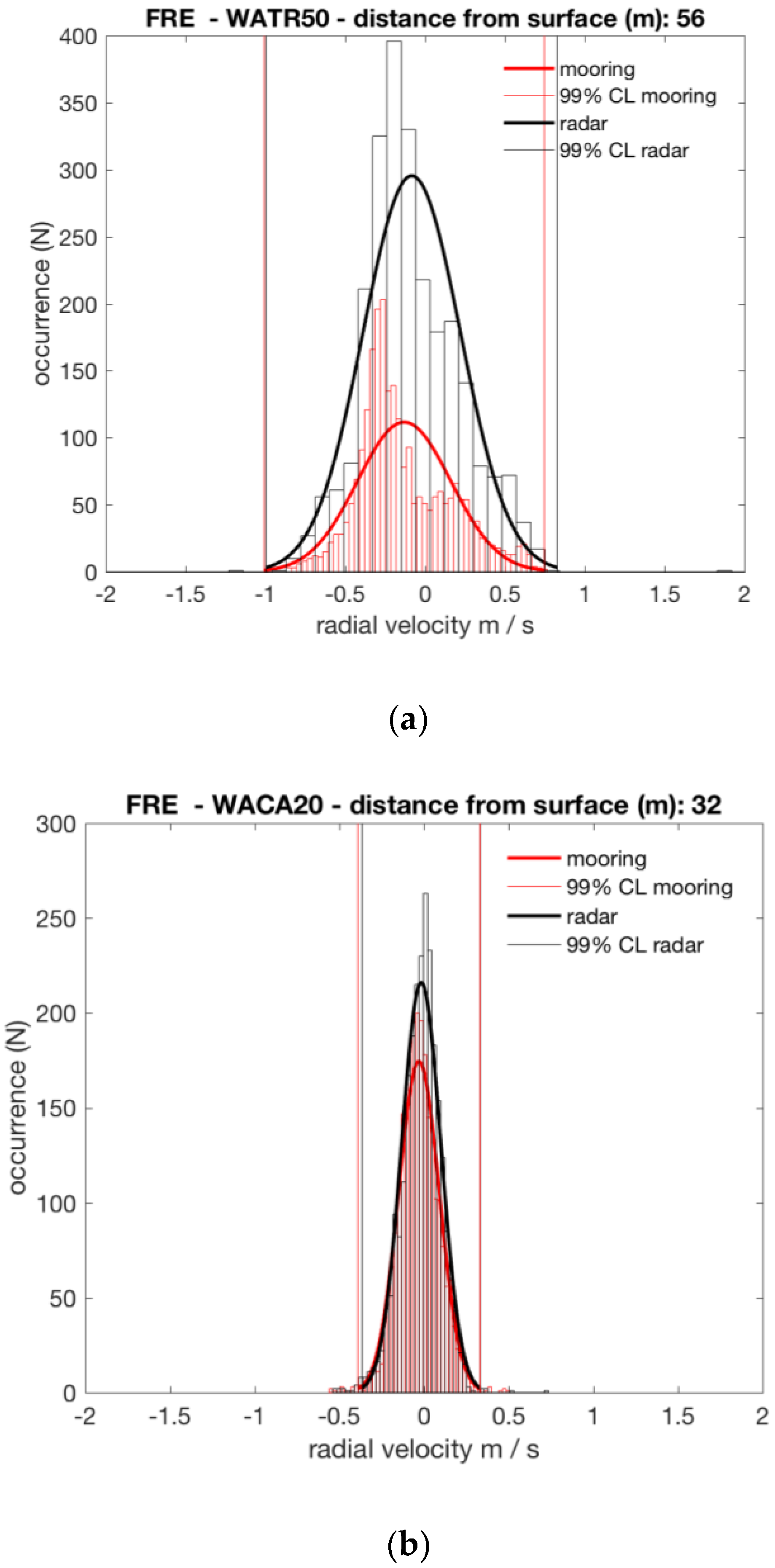
| WATR50 | 56 | 0.86/16.5 | 0.89/14.7 | 0.80/14.3 | 0.79/14.2 |
| WATR10 | 43 | 0.30/32.0 | 0.54/21.4 | 0.25/12.5 | 0.24/12.4 |
| WATR20 | 32 | 0.79/18.6 | 0.88/14.4 | 0.78/11.8 | 0.78/11.8 |
| WACA20 | 32 | 0.63/10.3 | 0.62/10.0 | 0.36/30.8 | 0.54/20.8 |
| WATR04 | 13 | 0.46/27.7 | 0.72/14.7 | 0.65/12.7 | 0.66/11.9 |
| WATR10 | 43 | 0.15/40.8 | 0.36/21.5 | 0.31/10.7 | 0.30/9.7 |
| Mooring | Distance from Surface (m) | FRE R/RMSD a | FRE R/RMSD b | GUI R/RMSD a | GUI R/RMSD b |
|---|---|---|---|---|---|
| NRSROT | 15 | 0.44/11.6 | 0.44/11.5 | 0.52/26.2 | 0.75/20.9 |
| WACA20 | 27 | 0.59/14.5 | 0.58/14.3 | 0.43/30.9 | 0.50/30.5 |
| WATR04 | 14 | 0.67/17.1 | 0.89/8.4 | 0.72/10.3 | 0.72/10.2 |
| WATR50 | 56 | 0.86/16.5 | 0.88/14.5 | 0.80/14.3 | 0.80/14.2 |
| WATR10 | 43 | 0.30/32.0 | 0.59/20.4 | 0.25/12.5 | 0.24/12.5 |
| WATR20 | 32 | 0.79/18.6 | 0.88/14.2 | 0.78/11.8 | 0.78/11.8 |
| WACA20 | 32 | 0.63/10.3 | 0.63/10.1 | 0.36/30.8 | 0.66/17.1 |
| WATR04 | 13 | 0.46/27.7 | 0.86/9.0 | 0.65/12.7 | 0.71/11.5 |
| WATR10 | 43 | 0.15/40.8 | 0.66/10.8 | 0.31/10.7 | 0.31/10.6 |
| Mooring | Distance from Surface (m) | FRE R/RMSD a | FRE R/RMSD b | GUI R/RMSD a | GUI R/RMSD b |
|---|---|---|---|---|---|
| NRSROT | 15 | 0.44/11.6 | 0.45/11.4 | 0.52/26.2 | 0.77/20.6 |
| WACA20 | 27 | 0.59/14.5 | 0.82/13.8 | 0.43/30.9 | 0.50/30.5 |
| WATR04 | 14 | 0.67/17.1 | 0.89/8.4 | 0.72/10.3 | 0.72/10.1 |
| WATR50 | 56 | 0.86/16.5 | 0.89/14.3 | 0.80/14.3 | 0.81/13.9 |
| WATR10 | 43 | 0.30/32.0 | 0.59/20.4 | 0.25/12.5 | 0.25/12.4 |
| WATR20 | 32 | 0.79/18.6 | 0.89/13.9 | 0.78/11.8 | 0.78/11.8 |
| WACA20 | 32 | 0.63/10.3 | 0.84/9.9 | 0.36/30.8 | 0.66/17.1 |
| WATR04 | 13 | 0.46/27.7 | 0.88/8.7 | 0.65/12.7 | 0.72/11.3 |
| WATR10 | 43 | 0.15/40.8 | 0.69/10.1 | 0.31/10.7 | 0.32/10.2 |
© 2018 by the authors. Licensee MDPI, Basel, Switzerland. This article is an open access article distributed under the terms and conditions of the Creative Commons Attribution (CC BY) license (http://creativecommons.org/licenses/by/4.0/).
Share and Cite
Cosoli, S.; Grcic, B.; De Vos, S.; Hetzel, Y. Improving Data Quality for the Australian High Frequency Ocean Radar Network through Real-Time and Delayed-Mode Quality-Control Procedures. Remote Sens. 2018, 10, 1476. https://doi.org/10.3390/rs10091476
Cosoli S, Grcic B, De Vos S, Hetzel Y. Improving Data Quality for the Australian High Frequency Ocean Radar Network through Real-Time and Delayed-Mode Quality-Control Procedures. Remote Sensing. 2018; 10(9):1476. https://doi.org/10.3390/rs10091476
Chicago/Turabian StyleCosoli, Simone, Badema Grcic, Stuart De Vos, and Yasha Hetzel. 2018. "Improving Data Quality for the Australian High Frequency Ocean Radar Network through Real-Time and Delayed-Mode Quality-Control Procedures" Remote Sensing 10, no. 9: 1476. https://doi.org/10.3390/rs10091476
APA StyleCosoli, S., Grcic, B., De Vos, S., & Hetzel, Y. (2018). Improving Data Quality for the Australian High Frequency Ocean Radar Network through Real-Time and Delayed-Mode Quality-Control Procedures. Remote Sensing, 10(9), 1476. https://doi.org/10.3390/rs10091476