A Long-Term Fine-Resolution Record of AVHRR Surface Temperatures for the Laurentian Great Lakes


Abstract
1. Introduction
2. Data and Methods
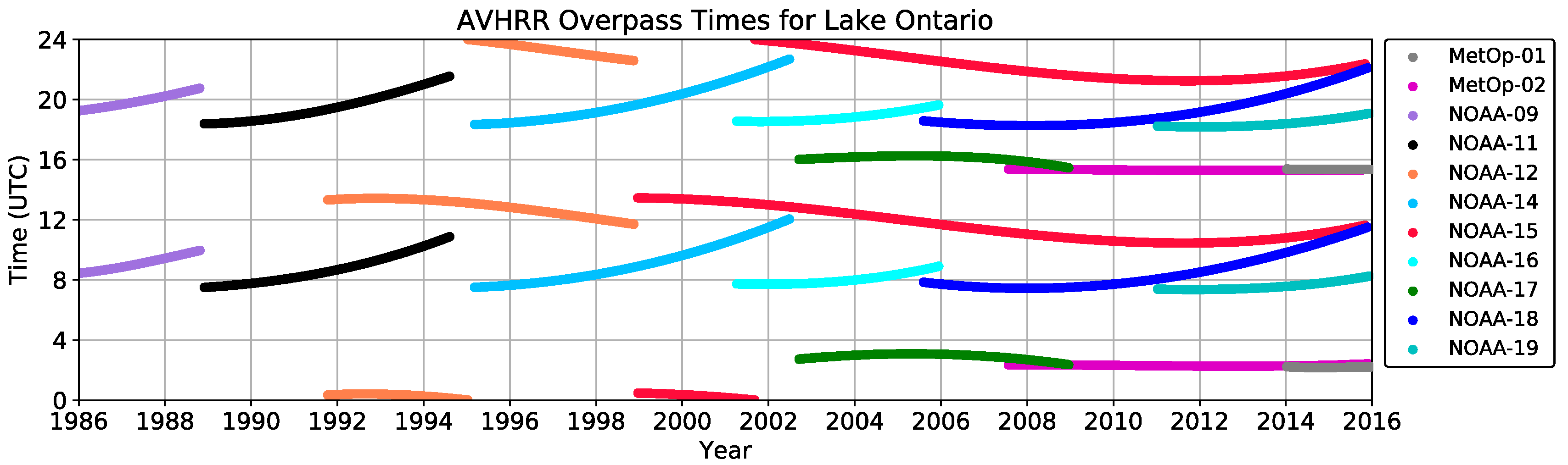
2.1. Datasets
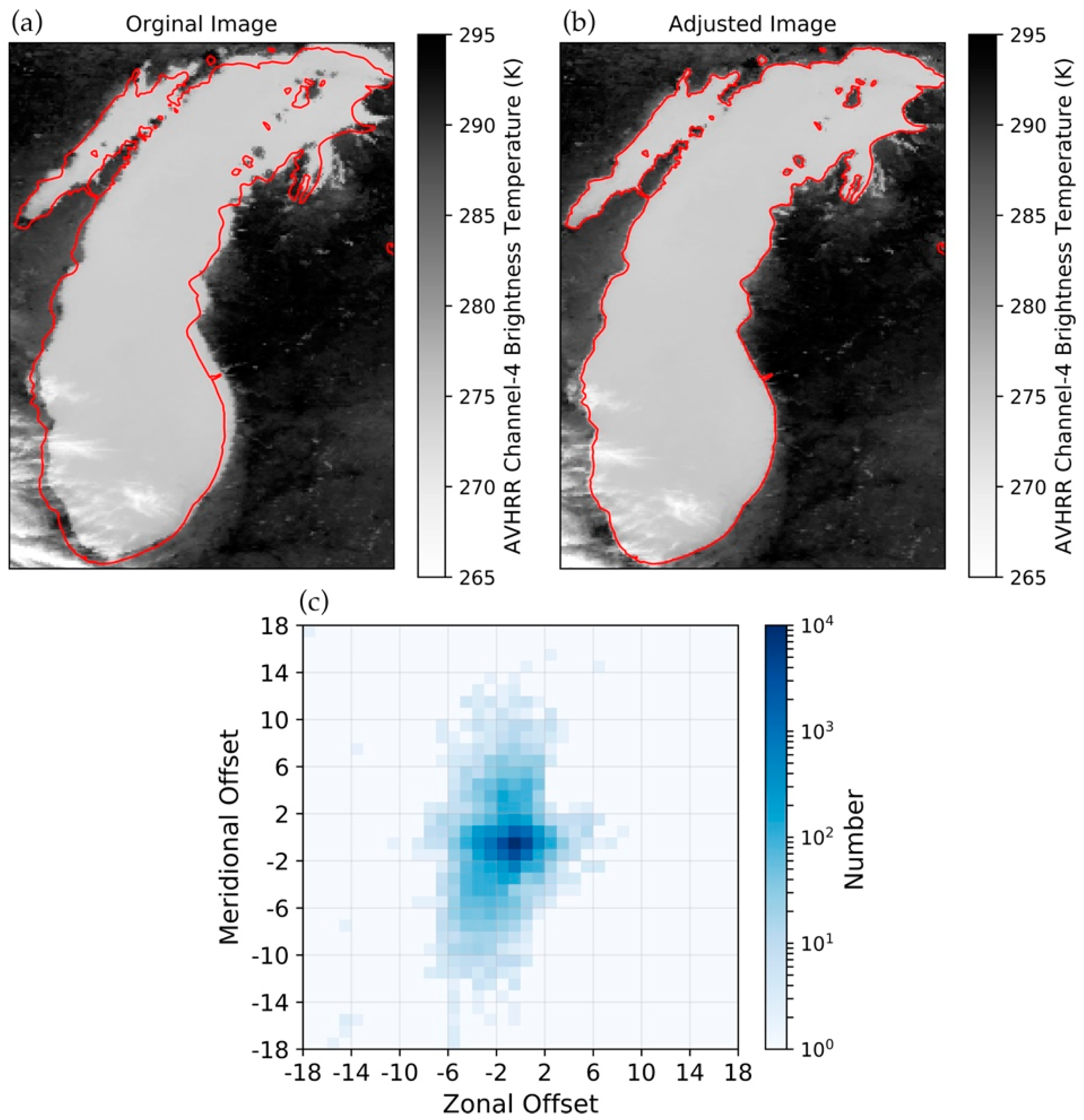
2.2. Georegistration Adjustments
2.3. Cloud, Ice, and Land Masking
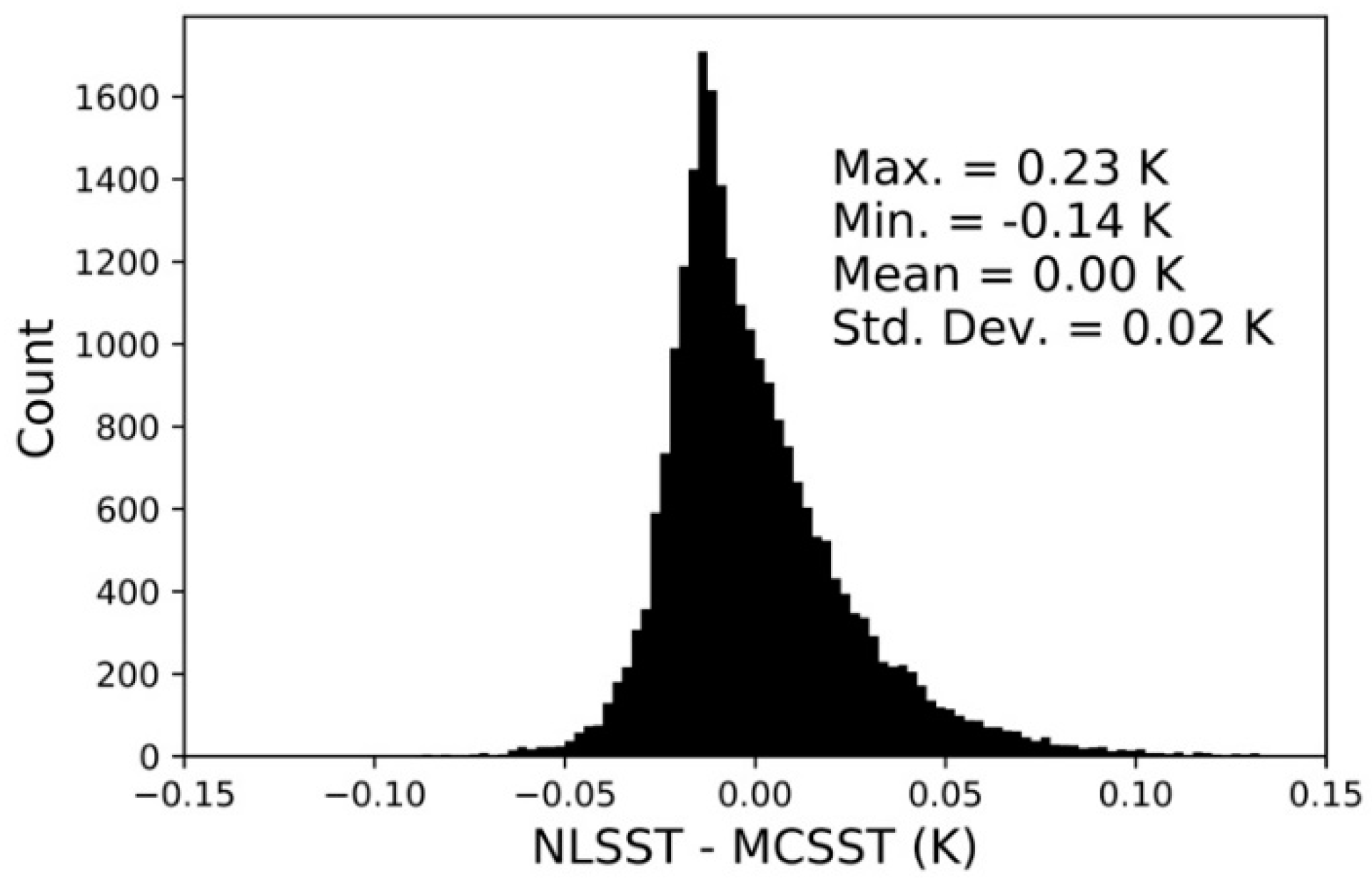
2.4. Lake Surface Water Temperature Calculation
2.5. Diurnal Correction
2.6. Gap-Filling
3. Results
3.1. Georegistration Adjustments
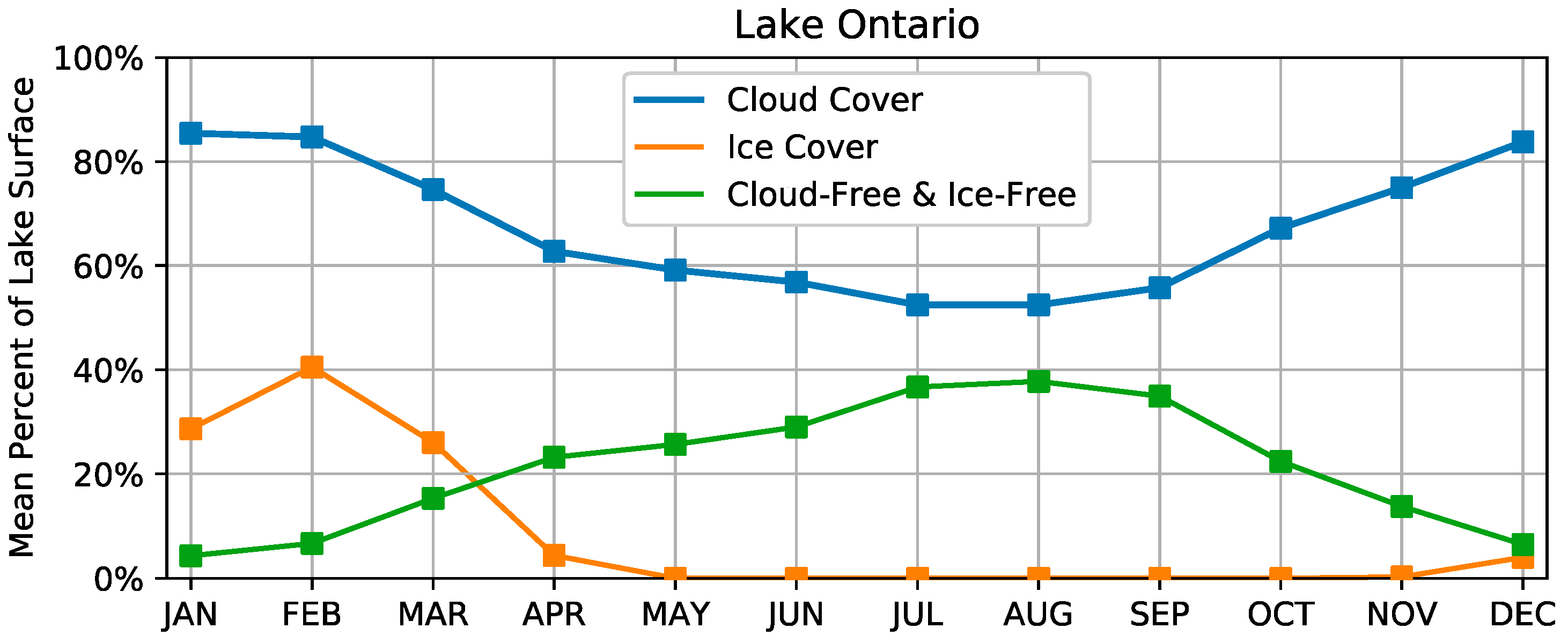
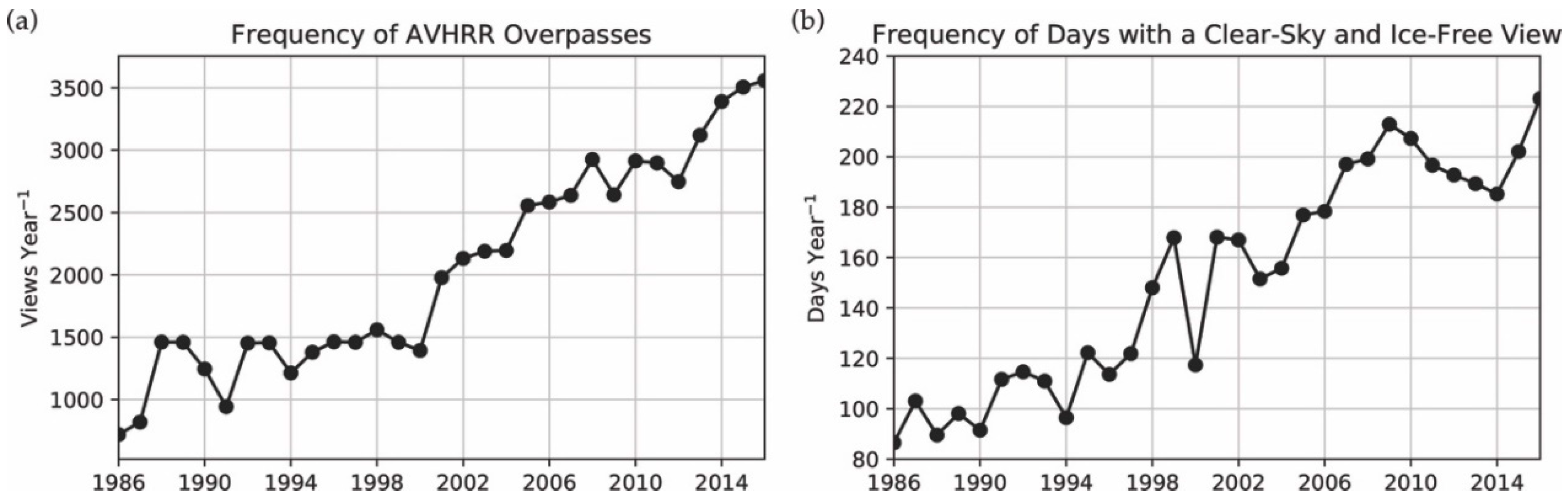
3.2. Cloud and Ice Masking
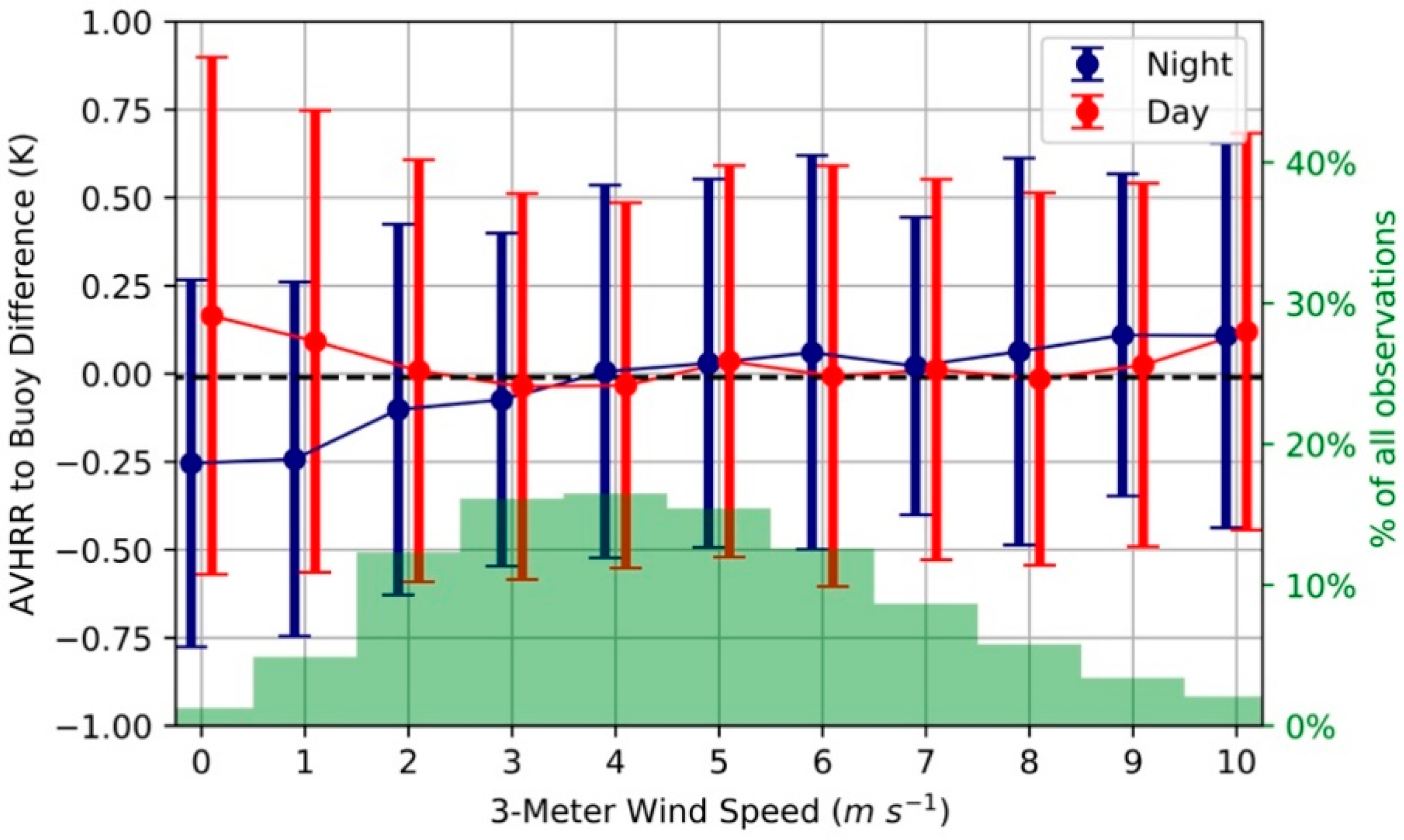
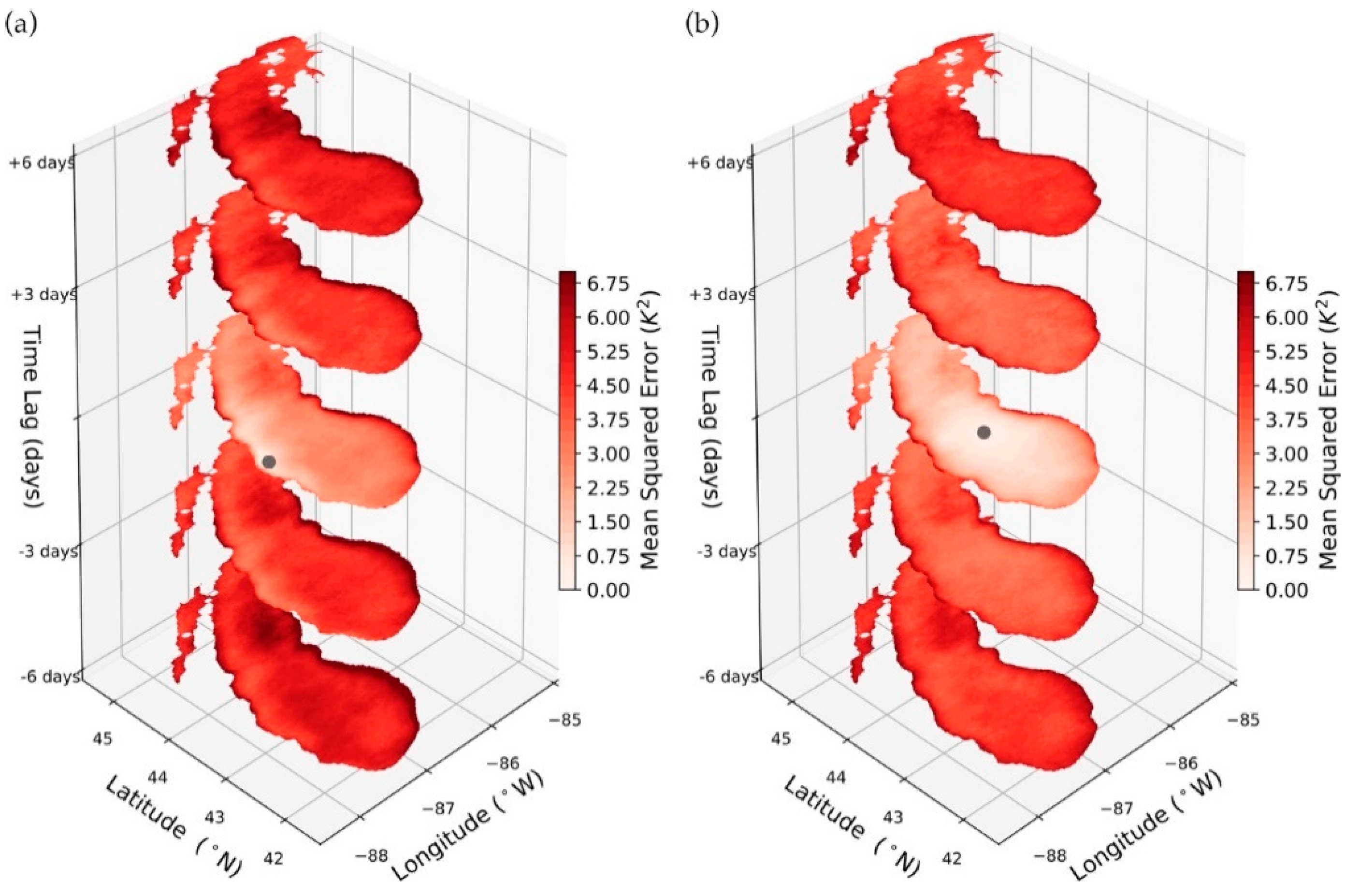
3.3. LSWT Error
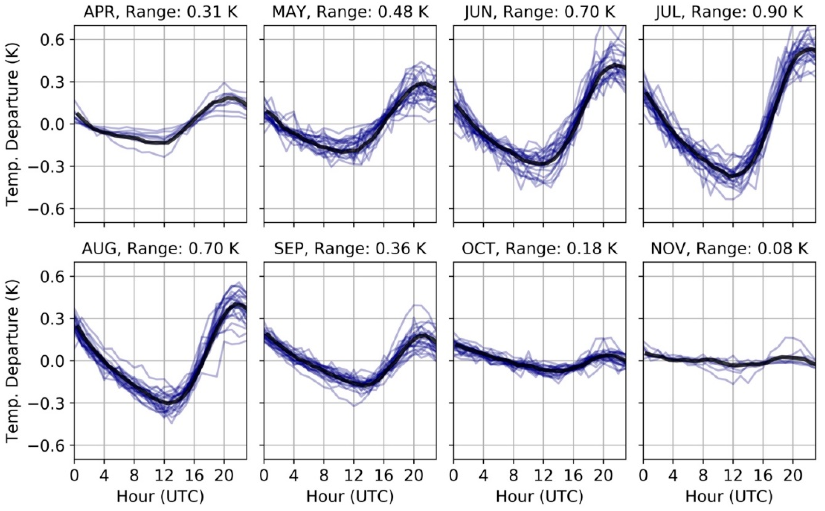
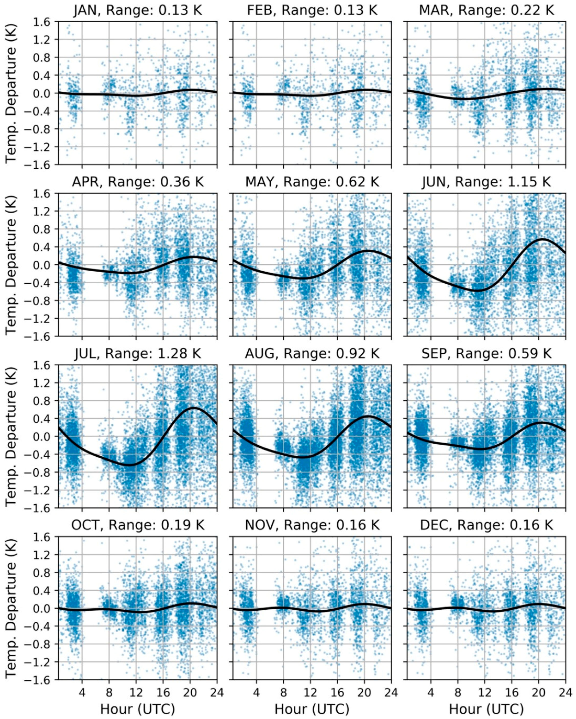
3.4. Diurnal Correction and Compositing
3.5. Gap Filling and Cross-Validation
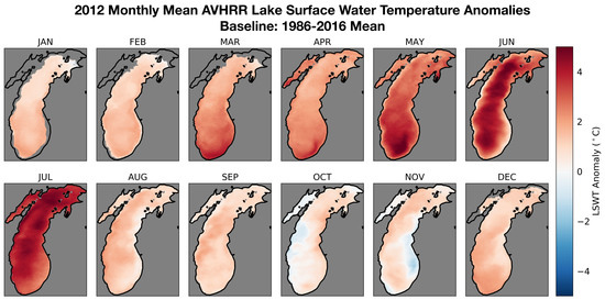
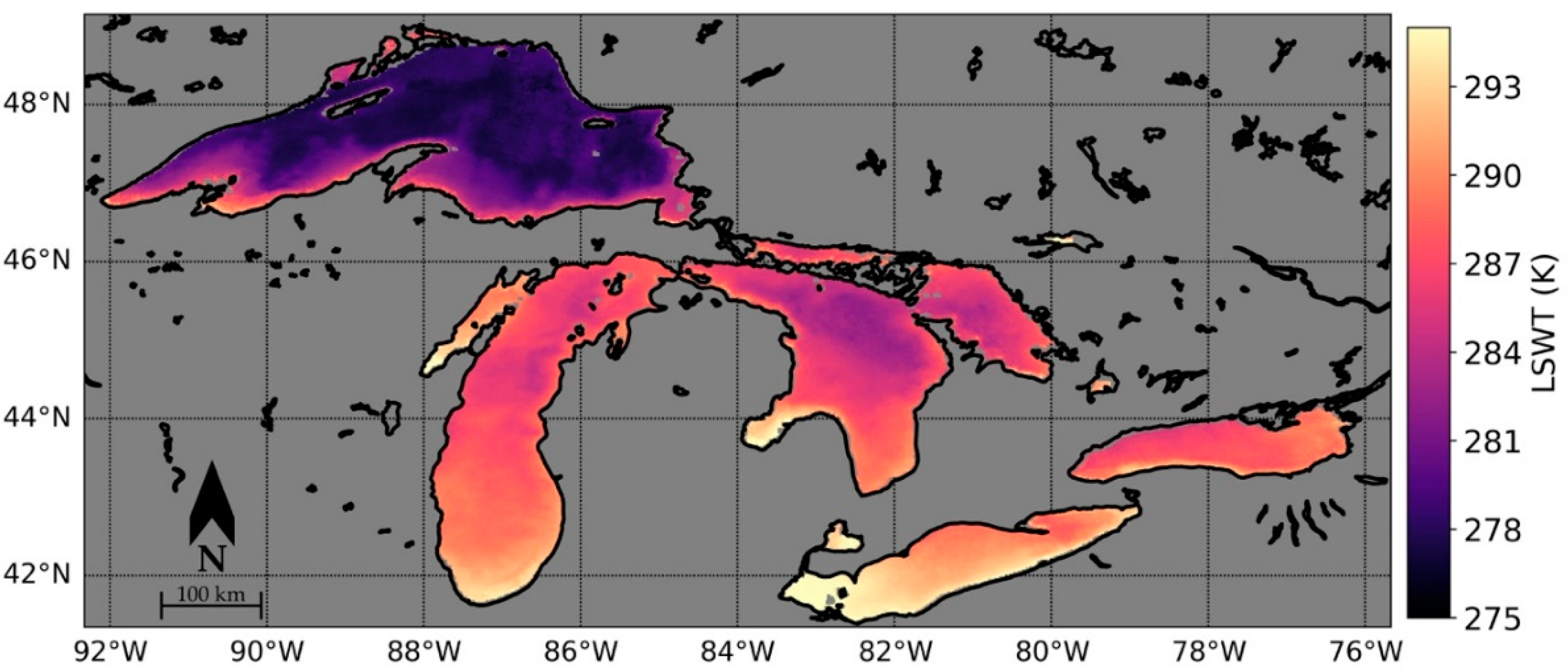
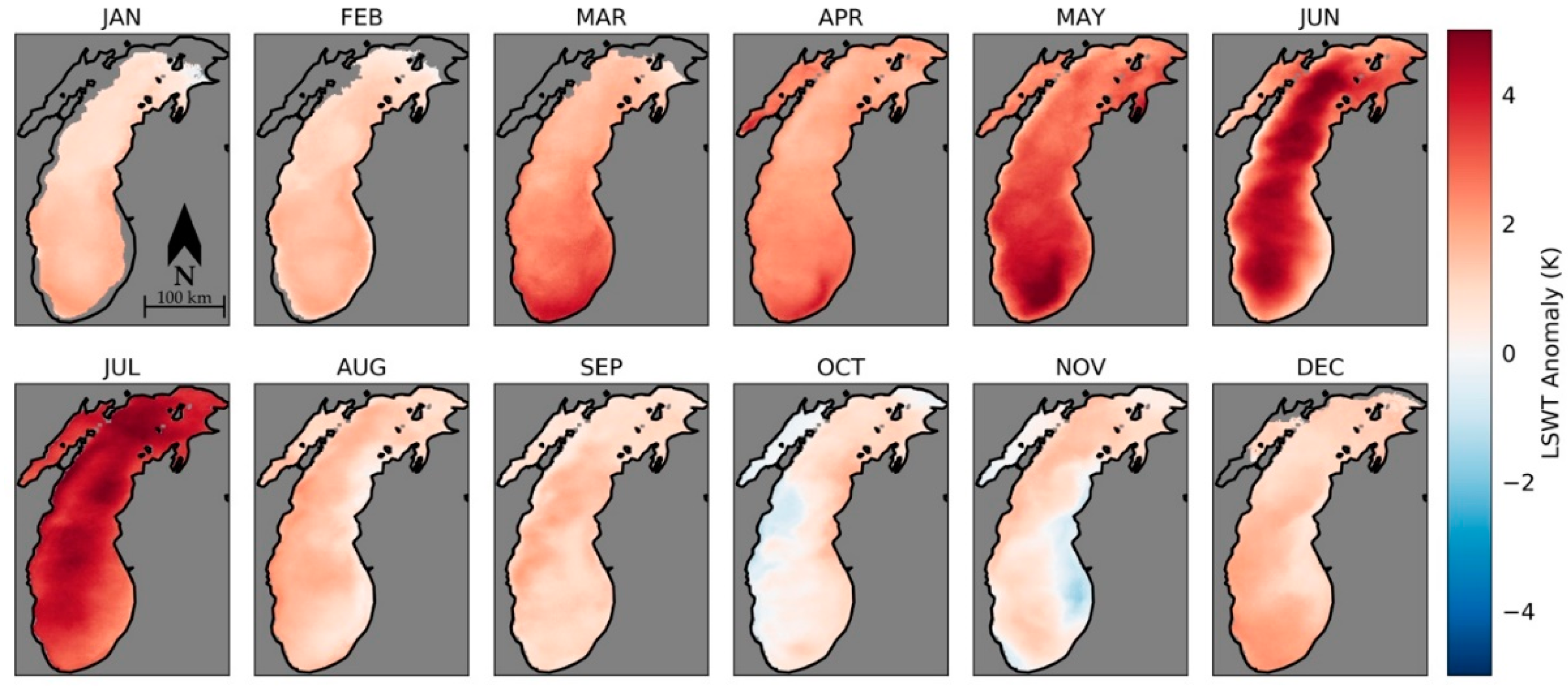
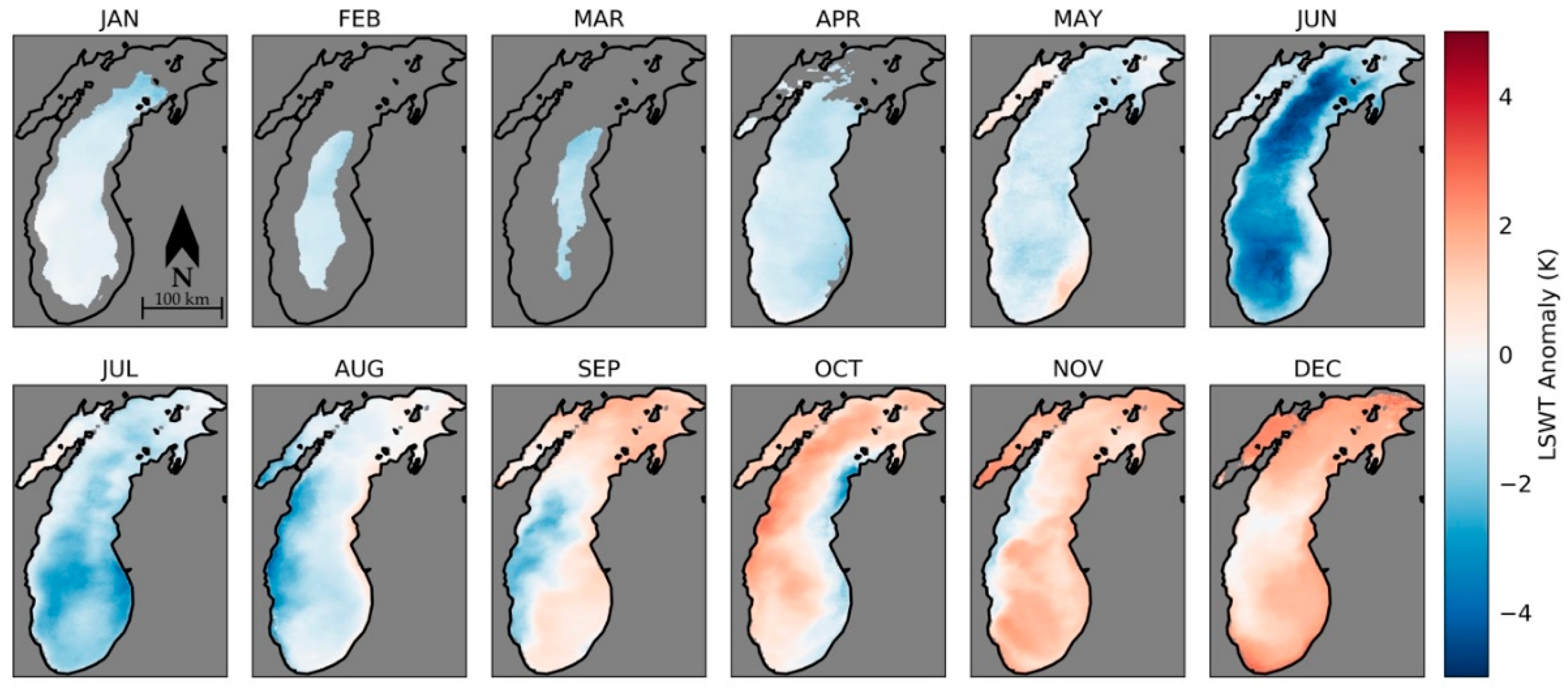
3.6. LSWT Spatial and Temporal Variation
4. Discussion
5. Conclusions
Author Contributions
Funding
Acknowledgments
Conflicts of Interest
Appendix A

| Platform | LSWT RMSE | Matchups |
|---|---|---|
| NOAA-9 | 0.690 K | 583 |
| NOAA-11 | 0.694 K | 1327 |
| NOAA-12 | 0.706 K | 1387 |
| NOAA-14 | 0.619 K | 2017 |
| NOAA-15 | 0.586 K | 6685 |
| NOAA-16 | 0.628 K | 1881 |
| NOAA-17 | 0.618 K | 1523 |
| NOAA-18 | 0.559 K | 3083 |
| NOAA-19 | 0.514 K | 3397 |
| MetOp-A | 0.541 K | 1227 |
| MetOp-B | 0.563 K | 4547 |
References
- O’Reilly, C.M.; Sharma, S.; Gray, D.K.; Hampton, S.E.; Read, J.S.; Rowley, R.J.; Schneider, P.; Lenters, J.D.; McIntyre, P.B.; Kraemer, B.M.; et al. Rapid and highly variable warming of lake surface waters around the globe. Geophys. Res. Lett. 2015, 42, 10773–10781. [Google Scholar] [CrossRef]
- Schneider, P.; Hook, S.J. Space observations of inland water bodies show rapid surface warming since 1985. Geophys. Res. Lett. 2010, 37. [Google Scholar] [CrossRef]
- Blumberg, A.F.; Di Toro, D.M. Effects of Climate Warming on Dissolved Oxygen Concentrations in Lake Erie. Trans. Am. Fish. Soc. 1990, 119, 210–223. [Google Scholar] [CrossRef]
- Gillooly, J.F. Effects of Size and Temperature on Metabolic Rate. Science 2001, 293, 2248–2251. [Google Scholar] [CrossRef] [PubMed]
- Kraemer, B.M.; Chandra, S.; Dell, A.I.; Dix, M.; Kuusisto, E.; Livingstone, D.M.; Schladow, S.G.; Silow, E.; Sitoki, L.M.; Tamatamah, R.; et al. Global patterns in lake ecosystem responses to warming based on the temperature dependence of metabolism. Glob. Chang. Biol. 2017, 23, 1881–1890. [Google Scholar] [CrossRef] [PubMed]
- Rahel, F.J.; Olden, J.D. Assessing the Effects of Climate Change on Aquatic Invasive Species. Conserv. Biol. 2008, 22, 521–533. [Google Scholar] [CrossRef] [PubMed]
- Smith, A.L.; Hewitt, N.; Klenk, N.; Bazely, D.R.; Yan, N.; Wood, S.; Henriques, I.; MacLellan, J.I.; Lipsig-Mummé, C. Effects of climate change on the distribution of invasive alien species in Canada: A knowledge synthesis of range change projections in a warming world. Environ. Rev. 2012, 20, 1–16. [Google Scholar] [CrossRef]
- Desai, A.R.; Austin, J.A.; Bennington, V.; McKinley, G.A. Stronger winds over a large lake in response to weakening air-to-lake temperature gradient. Nat. Geosci. 2009, 2, 855–858. [Google Scholar] [CrossRef]
- Magnuson, J.J. Historical Trends in Lake and River Ice Cover in the Northern Hemisphere. Science 2000, 289, 1743–1746. [Google Scholar] [CrossRef] [PubMed]
- Austin, J.A.; Colman, S.M. Lake Superior summer water temperatures are increasing more rapidly than regional air temperatures: A positive ice-albedo feedback. Geophys. Res. Lett. 2007, 34. [Google Scholar] [CrossRef]
- Kraemer, B.M.; Anneville, O.; Chandra, S.; Dix, M.; Kuusisto, E.; Livingstone, D.M.; Rimmer, A.; Schladow, S.G.; Silow, E.; Sitoki, L.M.; et al. Morphometry and average temperature affect lake stratification responses to climate change. Geophys. Res. Lett. 2015, 42, 4981–4988. [Google Scholar] [CrossRef]
- Winslow, L.A.; Read, J.S.; Hansen, G.J.A.; Rose, K.C.; Robertson, D.M. Seasonality of change: Summer warming rates do not fully represent effects of climate change on lake temperatures: Seasonal heterogeneity in lake warming. Limnol. Oceanogr. 2017, 62, 2168–2178. [Google Scholar] [CrossRef]
- Mason, L.A.; Riseng, C.M.; Gronewold, A.D.; Rutherford, E.S.; Wang, J.; Clites, A.; Smith, S.D.P.; McIntyre, P.B. Fine-scale spatial variation in ice cover and surface temperature trends across the surface of the Laurentian Great Lakes. Clim. Chang. 2016, 138, 71–83. [Google Scholar] [CrossRef]
- Woolway, R.I.; Merchant, C.J. Intralake Heterogeneity of Thermal Responses to Climate Change: A Study of Large Northern Hemisphere Lakes. J. Geophys. Res. Atmos. 2018, 123, 3087–3098. [Google Scholar] [CrossRef]
- Pareeth, S.; Salmaso, N.; Adrian, R.; Neteler, M. Homogenised daily lake surface water temperature data generated from multiple satellite sensors: A long-term case study of a large sub-Alpine lake. Sci. Rep. 2016, 6, 31251. [Google Scholar] [CrossRef] [PubMed]
- Wan, W.; Li, H.; Xie, H.; Hong, Y.; Long, D.; Zhao, L.; Han, Z.; Cui, Y.; Liu, B.; Wang, C.; et al. A comprehensive data set of lake surface water temperature over the Tibetan Plateau derived from MODIS LST products 2001–2015. Sci. Data 2017, 4, 170095. [Google Scholar] [CrossRef] [PubMed]
- Woolway, R.I.; Merchant, C.J. Amplified surface temperature response of cold, deep lakes to inter-annual air temperature variability. Sci. Rep. 2017, 7, 4130. [Google Scholar] [CrossRef] [PubMed]
- Wilson, R.C.; Hook, S.J.; Schneider, P.; Schladow, S.G. Skin and bulk temperature difference at Lake Tahoe: A case study on lake skin effect. J. Geophys. Res. Atmos. 2013, 118, 10332–10346. [Google Scholar] [CrossRef]
- Donlon, C.J.; Minnett, P.J.; Gentemann, C.; Nightingale, T.J.; Barton, I.J.; Ward, B.; Murray, M.J. Toward Improved Validation of Satellite Sea Surface Skin Temperature Measurements for Climate Research. J. Clim. 2002, 15, 353–369. [Google Scholar] [CrossRef]
- Schluessel, P.; Emery, W.J.; Grassl, H.; Mammen, T. On the bulk-skin temperature difference and its impact on satellite remote sensing of sea surface temperature. Geophys. Res. 1990, 95, 13341. [Google Scholar] [CrossRef]
- Minnett, P.J.; Smith, M.; Ward, B. Measurements of the oceanic thermal skin effect. Deep Sea Res. Part II Top. Stud. Oceanogr. 2011, 58, 861–868. [Google Scholar] [CrossRef]
- Webster, P.J.; Clayson, C.A.; Curry, J.A. Clouds, Radiation, and the Diurnal Cycle of Sea Surface Temperature in the Tropical Western Pacific. J. Clim. 1996, 9, 1712–1730. [Google Scholar] [CrossRef]
- Gentemann, C.L. Diurnal signals in satellite sea surface temperature measurements. Geophys. Res. Lett. 2003, 30. [Google Scholar] [CrossRef]
- Gentemann, C.L.; Minnett, P.J.; Le Borgne, P.; Merchant, C.J. Multi-satellite measurements of large diurnal warming events. Geophys. Res. Lett. 2008, 35. [Google Scholar] [CrossRef]
- Woolway, R.I.; Jones, I.D.; Maberly, S.C.; French, J.R.; Livingstone, D.M.; Monteith, D.T.; Simpson, G.L.; Thackeray, S.J.; Andersen, M.R.; Battarbee, R.W.; et al. Diel surface temperature range scales with lake size. PLoS ONE 2016, 11, 1–14. [Google Scholar] [CrossRef] [PubMed]
- Bordes, P.; Brunel, P.; Marsouin, A. Automatic Adjustment of AVHRR Navigation. J. Atmos. Ocean. Technol. 1992, 9, 15–27. [Google Scholar] [CrossRef]
- Moreno, J.F.; Melia, J. A method for accurate geometric correction of NOAA AVHRR HRPT data. IEEE Trans. Geosci. Remote Sens. 1993, 31, 204–226. [Google Scholar] [CrossRef]
- Baldwin, D.G.; Emery, W.J. A systematized approach to AVHRR image navigation. Ann. Glaciol. 1993, 17, 414–420. [Google Scholar] [CrossRef]
- Schwab, D.J.; Leshkevich, G.A.; Muhr, G.C. Automated Mapping of Surface Water Temperature in the Great Lakes. J. Great Lakes Res. 1999, 25, 468–481. [Google Scholar] [CrossRef]
- MacCallum, S.N.; Merchant, C.J. Surface water temperature observations of large lakes by optimal estimation. Can. J. Remote Sens. 2012, 38, 25–45. [Google Scholar] [CrossRef]
- Heidinger, A.K.; Foster, M.J.; Walther, A.; Zhao, X. The Pathfinder Atmospheres–Extended AVHRR Climate Dataset. Bull. Am. Meteorol. Soc. 2014, 95, 909–922. [Google Scholar] [CrossRef]
- Assel, R.A.; Norton, D.C.; Cronk, K.C. Great Lakes Ice Cover, First Ice, Last Ice, and Ice Duration: Winters 1973–2002; NOAA Technical Memorandum GLERL-121; NOAA Great Lakes Environmental Research Laboratory: Ann Arbor, MI, USA, 2002.
- Assel, R.A. Great Lakes Ice Cover Climatology Update: Winters 2003, 2004, and 2005; NOAA Technical Memorandum GLERL-135; NOAA Great Lakes Environmental Research Laboratory: Ann Arbor, MI, USA, 2005.
- Wang, J.; Assel, R.A.; Walterscheid, S.; Clites, A.H.; Bai, X. Great Lakes Ice Climatology Update, Winters 2006–2011, Description of the Digital Ice Cover Dataset; NOAA Technical Memorandum GLERL-155; NOAA Great Lakes Environmental Research Laboratory: Ann Arbor, MI, USA, 2012.
- Xu, F.; Ignatov, A. In situ SST Quality Monitor (iQuam). J. Atmos. Ocean. Technol. 2014, 31, 164–180. [Google Scholar] [CrossRef]
- Carroll, M.L.; DiMiceli, C.M.; Wooten, M.R.; Hubbard, A.B.; Sohlberg, R.A.; Townshend, J.R.G. MOD44W MODIS/Terra Land Water Mask Derived from MODIS and SRTM L3 Global 250m SIN Grid V006; NASA EOSDIS Land Process DAAC: Sioux Falls, SD, USA, 2017. [CrossRef]
- Heidinger, A.K.; Evan, A.T.; Foster, M.J.; Walther, A. A naive Bayesian cloud-detection scheme derived from Calipso and applied within PATMOS-x. J. Appl. Meteorol. Climatol. 2012, 51, 1129–1144. [Google Scholar] [CrossRef]
- Walton, C.C. Nonlinear Multichannel Algorithms for Estimating Sea Surface Temperature with AVHRR Satellite Data. J. Appl. Meteorol. 1988, 27, 115–124. [Google Scholar] [CrossRef]
- Walton, C.C.; Pichel, W.G.; Sapper, J.F.; May, D.A. The development and operational application of nonlinear algorithms for the measurement of sea surface temperatures with the NOAA polar-orbiting environmental satellites. J. Geophys. Res. Oceans 1998, 103, 27999–28012. [Google Scholar] [CrossRef]
- McMillin, L.M.; Crosby, D.S. Theory and validation of the multiple window sea surface temperature technique. J. Geophys. Res. 1984, 89, 3655. [Google Scholar] [CrossRef]
- Kilpatrick, K.A.; Podestá, G.P.; Evans, R. Overview of the NOAA/NASA advanced very high resolution radiometer Pathfinder algorithm for sea surface temperature and associated matchup database. J. Geophys. Res. 2001, 106, 9179–9197. [Google Scholar] [CrossRef]
- Foster, M.J.; Heidinger, A. PATMOS-x: Results from a Diurnally Corrected 30-yr Satellite Cloud Climatology. J. Clim. 2013, 26, 414–425. [Google Scholar] [CrossRef]
- Riffler, M.; Lieberherr, G.; Wunderle, S. Lake surface water temperatures of European Alpine lakes (1989–2013) based on the Advanced Very High Resolution Radiometer (AVHRR) 1 km data set. Earth Syst. Sci. Data 2015, 7, 1–17. [Google Scholar] [CrossRef]
- Cleveland, W.S. Robust Locally Weighted Regression and Smoothing Scatterplots. J. Am. Stat. Assoc. 1979, 74, 829–836. [Google Scholar] [CrossRef]
- Cleveland, W.S.; Devlin, S.J.; Grosse, E. Regression by local fitting: Methods, properties, and computational algorithms. J. Econ. 1988, 37, 87–114. [Google Scholar] [CrossRef]
- Alvera-Azcárate, A.; Barth, A.; Rixen, M.; Beckers, J.M. Reconstruction of incomplete oceanographic data sets using empirical orthogonal functions: Application to the Adriatic Sea surface temperature. Ocean Model. 2005, 9, 325–346. [Google Scholar] [CrossRef]
- Ackerman, S.A.; Heidinger, A.; Foster, M.J.; Maddux, B. Satellite Regional Cloud Climatology over the Great Lakes. Remote Sens. 2013, 5, 6223–6240. [Google Scholar] [CrossRef]
- Mesinger, F.; DiMego, G.; Kalnay, E.; Mitchell, K.; Shafran, P.C.; Ebisuzaki, W.; Jović, D.; Woollen, J.; Rogers, E.; Berbery, E.H.; et al. North American Regional Reanalysis. Bull. Am. Meteorol. Soc. 2006, 87, 343–360. [Google Scholar] [CrossRef]
- Plattner, S.; Mason, D.M.; Leshkevich, G.A.; Schwab, D.J.; Rutherford, E.S. Classifying and Forecasting Coastal Upwellings in Lake Michigan Using Satellite Derived Temperature Images and Buoy Data. J. Great Lakes Res. 2006, 32, 63–76. [Google Scholar] [CrossRef]
- Reynolds, R.W. Impact of Mount Pinatubo Aerosols on Satellite-derived Sea Surface Temperatures. J. Clim. 1993, 6, 768–774. [Google Scholar] [CrossRef]
- McCormick, M.P.; Thomason, L.W.; Trepte, C.R. Atmospheric effects of the Mt Pinatubo eruption. Nature 1995, 373, 399–404. [Google Scholar] [CrossRef]
- Dudhia, A. Noise characteristics of the AVHRR infrared channels. Int. J. Remote Sens. 1989, 10, 637–644. [Google Scholar] [CrossRef]
- Warren, D. AVHRR channel-3 noise and methods for its removal. Int. J. Remote Sens. 1989, 10, 645–651. [Google Scholar] [CrossRef]
- Li, X.; Pichel, W.; Clemente-Colón, P.; Krasnopolsky, V.; Sapper, J. Validation of coastal sea and lake surface temperature measurements derived from NOAA/AVHRR data. Int. J. Remote Sens. 2001, 22, 1285–1303. [Google Scholar] [CrossRef]
- Binding, C.E.; Greenberg, T.A.; Watson, S.B.; Rastin, S.; Gould, J. Long term water clarity changes in North America’s Great Lakes from multi-sensor satellite observations. Limnol. Oceanogr. 2015, 60, 1976–1995. [Google Scholar] [CrossRef]


| Platform | Number of Adjustments | Zonal Offsets | Meridional Offsets | ||
|---|---|---|---|---|---|
| Mean | Std. Dev. | Mean | Std. Dev. | ||
| NOAA-9 | 1205 (1117) | −0.92 (−0.80) | 1.76 (1.65) | −1.51 (1.76) | 2.85 (1.73) |
| NOAA-11 | 1809 (1754) | −1.23 (−0.45) | 1.82 (1.49) | −2.52 (1.92) | 3.15 (3.04) |
| NOAA-12 | 2355 (2694) | −1.22 (−0.19) | 1.72 (1.30) | −2.37 (2.05) | 3.47 (3.16) |
| NOAA-14 | 2994 (2793) | −1.21 (0.03) | 1.58 (1.19) | −0.15 (0.22) | 1.05 (1.10) |
| NOAA-15 | 7381 (7534) | −0.24 (0.12) | 1.46 (1.52) | −0.14 (−0.14) | 1.13 (1.25) |
| NOAA-16 | 2183 (1981) | −0.82 (−0.36) | 1.07 (1.26) | 0.06 (−0.11) | 0.97 (1.10) |
| NOAA-17 | 1862 (2868) | −0.36 (−0.02) | 0.91 (1.16) | −0.37 (0.28) | 0.80 (0.96) |
| NOAA-18 | 4498 (4203) | −0.08 (0.18) | 1.08 (1.34) | 0.15 (−0.18) | 1.00 (1.25) |
| NOAA-19 | 3110 (2965) | 0.11 (0.19) | 1.25 (1.34) | −0.19 (−0.13) | 1.11 (1.28) |
| MetOp-A | 3432 (3366) | 0.18 (0.20) | 1.01 (1.10) | −0.71 (0.23) | 1.00 (1.17) |
| MetOp-B | 1103 (1237) | 0.27 (0.04) | 1.08 (1.20) | −0.92 (0.33) | 1.02 (1.17) |
| Gap Filling Method | RMSE | Bias | Correlation Coefficient (ρ) |
|---|---|---|---|
| LWA | 1.57 K | 0.10 K | 0.67 |
| LOESS | 1.26 K | 0.04 K | 0.75 |
| LOESS + Selective LWA | 1.10 K | 0.05 K | 0.86 |
© 2018 by the authors. Licensee MDPI, Basel, Switzerland. This article is an open access article distributed under the terms and conditions of the Creative Commons Attribution (CC BY) license (http://creativecommons.org/licenses/by/4.0/).
Share and Cite
White, C.H.; Heidinger, A.K.; Ackerman, S.A.; McIntyre, P.B. A Long-Term Fine-Resolution Record of AVHRR Surface Temperatures for the Laurentian Great Lakes. Remote Sens. 2018, 10, 1210. https://doi.org/10.3390/rs10081210
White CH, Heidinger AK, Ackerman SA, McIntyre PB. A Long-Term Fine-Resolution Record of AVHRR Surface Temperatures for the Laurentian Great Lakes. Remote Sensing. 2018; 10(8):1210. https://doi.org/10.3390/rs10081210
Chicago/Turabian StyleWhite, Charles H., Andrew K. Heidinger, Steven A. Ackerman, and Peter B. McIntyre. 2018. "A Long-Term Fine-Resolution Record of AVHRR Surface Temperatures for the Laurentian Great Lakes" Remote Sensing 10, no. 8: 1210. https://doi.org/10.3390/rs10081210
APA StyleWhite, C. H., Heidinger, A. K., Ackerman, S. A., & McIntyre, P. B. (2018). A Long-Term Fine-Resolution Record of AVHRR Surface Temperatures for the Laurentian Great Lakes. Remote Sensing, 10(8), 1210. https://doi.org/10.3390/rs10081210