Article

A Phenology-Based Method to Map Cropping Patterns under a Wheat-Maize Rotation Using Remotely Sensed Time-Series Data

1
Shaanxi Key Laboratory of Earth Surface System and Environmental Carrying Capacity, Northwest University, Xi’an 710127, China
2
College of Urban and Environmental Science, Northwest University, Xi’an 710127, China
3
State Key Laboratory of Earth Surface Processes and Resource Ecology, Beijing Normal University, Beijing 100875, China
4
Institute of Surveying, Remote Sensing and Land Information, University of Natural Resources and Life Sciences (BOKU), Peter Jordan Strasse 82, Vienna 1190, Austria
5
School of Mining and Geomatics, Hebei University of Engineering, Handan 056038, China
6
State Key Laboratory of Remote Sensing Science, Jointly Sponsored by Beijing Normal University and Institute of Remote Sensing and Digital Earth of Chinese Academy of Sciences, Beijing 100875, China
*
Author to whom correspondence should be addressed.
Remote Sens. 2018, 10(8), 1203; https://doi.org/10.3390/rs10081203
Submission received: 15 July 2018 / Revised: 28 July 2018 / Accepted: 28 July 2018 / Published: 31 July 2018
(This article belongs to the Section Remote Sensing in Agriculture and Vegetation)

Abstract

:
Agricultural land use and cropping patterns are closely related to food production, soil degradation, water resource management, greenhouse gas emission, and regional climate alterations. Methods for reliable and cost-efficient mapping of cropping pattern, as well as their changes over space and time, are therefore urgently needed. To cope with this need, we developed a phenology-based method to map cropping patterns based on time-series of vegetation index data. The proposed method builds on the well-known ‘threshold model’ to retrieve phenological metrics. Values of four phenological parameters are used to identify crop seasons. Using a set of rules, the crop season information is translated into cropping pattern. To illustrate the method, cropping patterns were determined for three consecutive years (2008–2010) in the Henan province of China, where reliable validation data was available. Cropping patterns were derived using eight-day composite MODIS Enhanced Vegetation Index (EVI) data. Results show that the proposed method can achieve a satisfactory overall accuracy (~84%) in extracting cropping patterns. Interestingly, the accuracy obtained with our method based on MODIS EVI data was comparable with that from Landsat-5 TM image classification. We conclude that the proposed method for cropland and cropping pattern identification based on MODIS data offers a simple, yet reliable way to derive important land use information over large areas.

Graphical Abstract

1. Introduction

The planting sequence and spatial arrangement of crops in a given area defines its cropping pattern [1]. Cropping patterns are closely related to land use intensity, food production, soil degradation, water resource management, greenhouse gas emission and regional climate [2]. For example, inappropriate changes of cropping patterns may lead to soil degradation, water resources shortage and regional climate alterations [3,4]. Cropping patterns are also a major factor influencing greenhouse gas (GHG) emission from cultivated areas [5,6]. Indeed, as shown by Snyder et al. [7] and Wanyama et al. [8], croplands are the main source of direct GHG emissions from terrestrial ecosystems, such as CH4 and N2O, via fertilizer production and crop cultivation.
As the global population steadily grows, and cities and settlements expand, global cropland decreases, while at the same time natural resources are redistributed and land is converted to cropland [9]. Accordingly, cropping patterns also change. To achieve global food security, a so-called “sustainable intensification” has been proposed [10]. The challenge is to increase agricultural productivity without expanding agricultural land while minimizing environmental impacts. Hence, cropping patterns should be mapped timely and accurately to inform stakeholders and decision-makers [10,11]. Any proposed algorithm should also be applicable back in time, in order to permit comparison between current and historic cropping pattern.
Unfortunately, current land cover products derived from Earth Observation (EO) data do not provide sufficient details on cropland use and cropping patterns [2,12]. For illustration, a list of widely used (global) land cover products is provided in Table 1. The table highlights the fact that currently available land cover products mainly focus on cropland extent while lacking crucial information regarding cropping intensities and cropping patterns. Thus, there is a clear need for better information on the area and distribution of cropping patterns at regional scales [2]. On the other hand, information on cropland extent is more readily available, albeit not always consistent among datasets [13,14].
Remote sensing is probably the most efficient way to monitor agricultural land use characteristics such as cropland extent, cultivated crop types and cropping patterns over large areas [9,36,37,38,39]. Depending on the scale and scope of the application, both multi-temporal high-resolution data as well as coarse resolution time series contain relevant information regarding cropland extent, crop types and cropping patterns [25,40,41,42,43]. Approaches involving cloud-agnostic microwave data—possibly fused with optical data—are particularly beneficial in cloud-prone areas [44,45].
To derive cropping pattern, several alternatives exist [2]. One possible solution is to first acquire a few very high (metric to deca-metric) resolution images within the crop growing season. These images are used to identify different crops. Classical supervised land cover mapping techniques are appropriate for this task [46,47,48]. Cropping patterns are subsequently derived by combining crop maps from different growing seasons [49]. Although reliable results can be obtained [50], such approaches are generally very time consuming and difficult to realize for large areas. To acquire the necessary cloud-free images, weather conditions, combined with insufficient revisit frequencies of most deca-metric resolution satellites, constitute the main difficulty. Although data availability changed recently with ESA’s launch of two twin Sentinel-2 satellites (10m data at 5-daily revisit frequency), such dense high-resolution datasets are not available for retrospective analyses.
Alternatively, it is possible to identify cropping patterns through analysis of lower resolution EO time series. Such data are usually acquired with very high revisit frequency (e.g., with daily revisits) [12]. High revisit EO data are for example provided by moderate-resolution Imaging Spectroradiometer (MODIS) and Advanced Very High-Resolution Radiometer (AVHRR) sensors. In this way, most cloud issues can be avoided. Currently, however, such sensors only provide low spatial resolution (hecto- to kilometric). Using such coarse resolution EO time series, information about cropland use is extracted by examining the number of peaks in a vegetation index time series. The premise of this “peak-counting method” is that vegetation index dynamics of cropland correspond well to the growing cycles of crops, such as seeding, heading, maturing and senescence [51]. For example, vegetation index time series of single cropping presents only one growth cycle per year, while that of double cropping presents two cycles [52,53]. Hence, cropping patterns are identified by examining the periodic variations in the vegetation index time series. Sakamoto et al. [54], for example, studied rice cropping systems in the Mekong Delta from 2000 to 2005 by detecting the peaks in wavelet-filtered Enhanced Vegetation Index (EVI) curves. Their results indicated that the extent of triple cropping in An Giang, Vietnam, expanded yearly. Using a similar method, Galford et al. [55] found that there were 320,000 ha of native vegetation and pastures converted to cropland and 200,000 ha of single-cropped cropland converted to double cropping from 2000 to 2005 in the southwestern Brazilian Amazon. Lv and Liu [56] detected peaks in a HANTS-filtered NDVI time series, and found that double and triple cropping systems were commonly employed in the Chao Phraya Basin of Thailand.
Although peak-counting using coarse resolution EO time series is widely used, the approach suffers from at least three main drawbacks that limit its usability over large areas:
  • difficulties to detect crop cycles in the presence of sensor noise
  • difficulties to distinguish crop-related (temporal) signatures from non-agricultural vegetation
  • difficulties to deal with cropping patterns spanning multiple years
First, peak-counting is notably sensitive to noise in the vegetation index time series. Even after filtering and pre-processing, noise-related peaks may still be present in the data (Figure 1). Compared with crops, natural vegetation tends to have more plausible peaks because of its generally longer season length. Noise often causes (biased) errors when counting the number of peaks (e.g., overestimation). To identify the ‘true’ peaks in a vegetation curve, several criteria have been proposed. For example, Sakamoto et al. [54,57] considered that two peaks within less than 60 days should belong to the same growth period, as a typical rice growth cycle in the Mekong Delta lasts at least 80 days. Galford et al. [55] investigated cropping patterns in Brazil. When two or three peaks were detected within one year, they regarded the first “minor” peaks as caused by the early green-up of weeds or other green covers planted before crops. Obviously, such prior knowledge and extra constraints depend on personal experience and regional characteristics. As climate, soils and farming practices differ from region to region, such constraints are hard to generalize and thus not easily applicable for all areas [2]. The same problems also apply to curve fitting approaches as for example implemented in the widely used TIMESAT software [58]. Although curve fitting minimizes the impact of high frequency noise, user inputs are needed to specify the regional context and to constrain the algorithm [59].
With respect to the second above-mentioned limitation, one has to note that peak-counting methods usually cannot distinguish natural vegetation from crops, or no-cropping areas from fallow cropland. The difficulty arises because these land cover types may have the same number of peaks. As shown in Figure 1, both single cropping and natural vegetation present one season per year, with very similar amplitude. The only noticeable difference is the season length.
Finally, peaks in vegetation index curves only inform about the yearly crop planting frequency, while the cropping pattern is strictly speaking a multi-year phenomenon. For example, in some part of the North and Northwest China, farmers cultivate three crops in every two-year period due to local water and climate conditions [60] (Figure 1c). Crops such as sugarcane, on the other hand, are harvested only after 1.5 to 2.5 years, leading to growth cycles extending over multiple years [61]. Consequently, crop planting frequency in the current year may be different from that in the next year, while the general cropping pattern remains unchanged over many years or even decades. A number of prominent cropping patterns in North China are exemplified in Figure 1 to further illustrate the problem.
To identify cropping patterns in a robust and cost-efficient way across large areas and potentially in retrospective, this paper proposes a simple phenology-based cropping pattern (PBCP) mapping method. The proposed method identifies crop seasons and inter-seasons from smoothed EVI time series based on four phenological parameters. It first derives the number of crop seasons per year (i.e., cropping index) as well as cropland extent. Ultimately, using a set of decision rules based on the observed cropping indexes in three consecutive years embracing the year of interest, the cropping patterns are determined.

2. Study Area and Data
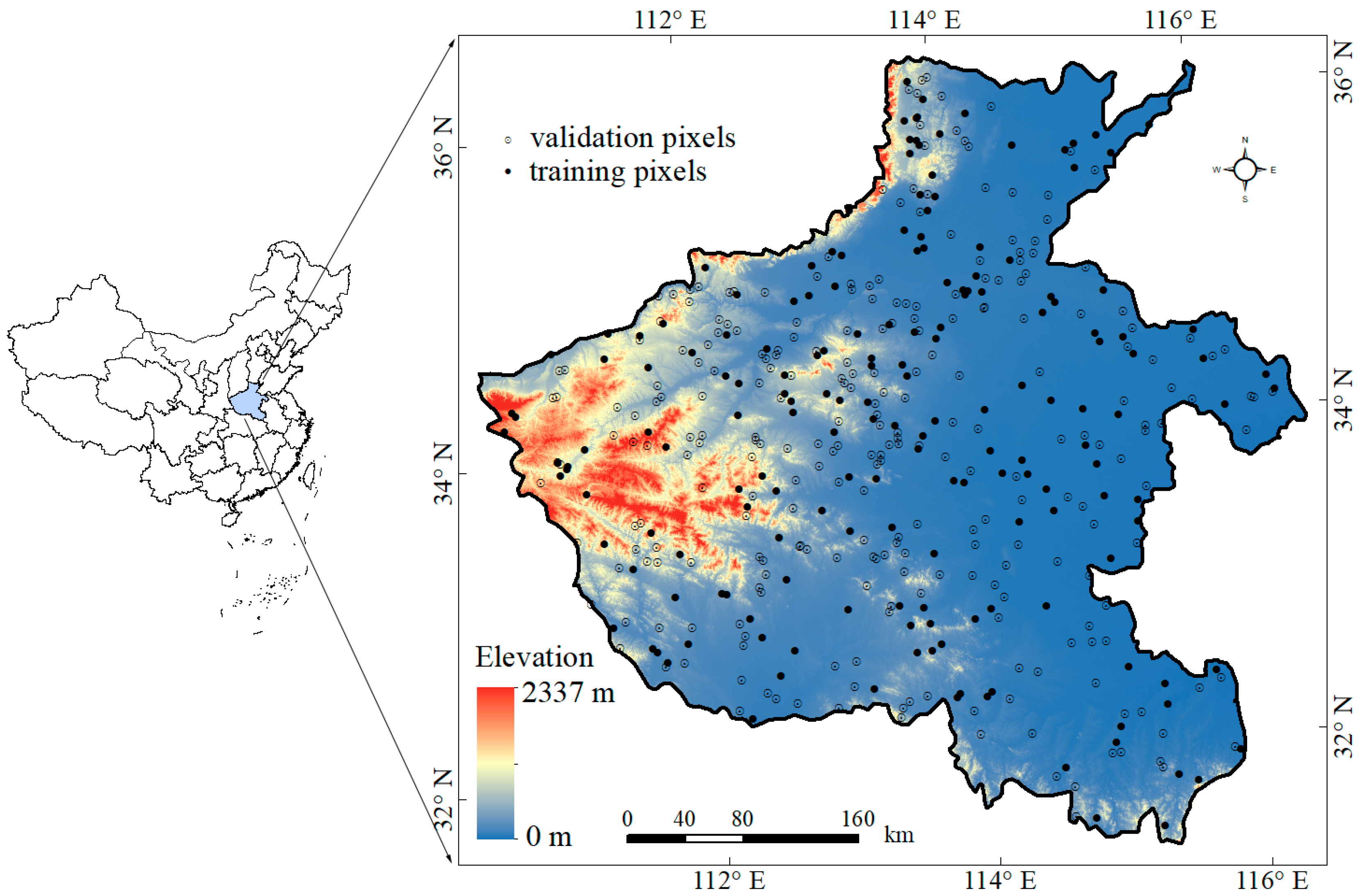
2.1. Study Area

To test and evaluate the approach, the Henan province of China was selected. The Henan province is located in the central part of China and lies in the mid-lower reach of the Yellow River with a total land area of 16 million ha (Figure 2). The eastern and central parts of Henan lie in the North China Plain, while the west and south regions are mountainous. The geographical and climate conditions are very favorable for crop cultivation. The major crops planted in Henan are winter wheat, maize, soybean and cotton, with winter wheat-summer maize rotation as the dominant cropping practice. According to the China Statistical Yearbook [62], the cultivated area in Henan was 8.1 million ha by the end of 2015, with a total grain crop yield of 60.67 million tons. According to this data, Henan province ranks as the second grain-producing province in China.

2.2. MODIS Data

The 8-day composited MODIS09A1 (V005) product provided by the International Scientific Data Service Platform, Computer Network Information Center, Chinese Academy of Sciences (http://datamirror.csdb.cn) covering Henan Province during 2008–2010 was used in this study. The spatial resolution of this data is 500 m. EVI was chosen to map cropping patterns because it has a greater dynamic range compared to NDVI and can capture crop phenological dynamics without reaching saturation [63]. The period between 2008 and 2010 was selected, as for this time period good training and validation data were available.
To minimize noise impacts and to reconstruct high-quality EVI time series, the changing-weight filter method proposed by Zhu et al. [64] was used. The method can effectively preserve the curve shape as well as the timing and the amplitude of the local maxima/minima in vegetation index time series. Preserving the integrity of phenology for multiple growth cycles is an important prerequisite of our approach. Alternative filter techniques exist (e.g., Atkinson et al. [65]) but were not evaluated here.

2.3. Landsat Images

Several cloudless Landsat-5 TM images were acquired to assist in identifying the crop growing seasons and validate the cropping index mapping accuracy. The TM images utilized in this paper are listed in Table 2.

2.4. Crop Calendars

To assist in setting proper thresholds for phenological parameters of the new method, a crop calendar from 2010 was used (Table 3). The underlying data were acquired from the database provided by Ministry of Agriculture and Rural Affairs of the People’s Republic of China (http://www.zzys.moa.gov.cn/). Winter wheat is usually sown in October, overwinters from late December to the next February and greens up in late February. In spring, winter wheat starts growing rapidly and is finally harvested in mid-June. Summer maize, soybean and peanut generally present very similar calendars. These crops are sown in June and harvested in late September to early October. Cotton, on the other hand, has a prolonged growing cycle compared to other crops. It is sown in early April and can be harvested many times from September to October. The typical crop season length of all crops is about 100–120 days, if one excludes the pre-winter growing of winter wheat.

2.5. Cropland Maps

To evaluate the quality of our proposed method with respect to the estimated cropland extent, three cropland layers derived from well-known global land cover products were considered:
  • 250 m Global Cropland Extent (GCE) product [25]. The GCE product maps global croplands independently, mainly based on MOD09 Collection 5 product covering 2000–2008.
  • 300 m GlobCover 2009 product [19]. To derive cropland extent, class 11 (post-flooding or irrigated croplands), class 14 (rainfed croplands) and class 20 (mosaic cropland (50–70%)/vegetation (grassland/shrubland/forest) (20–50%)) were combined.
  • 500 m MODIS IGBP land cover map for 2009 [16]. MODIS IGBP land cover permits a direct extraction of cropland.
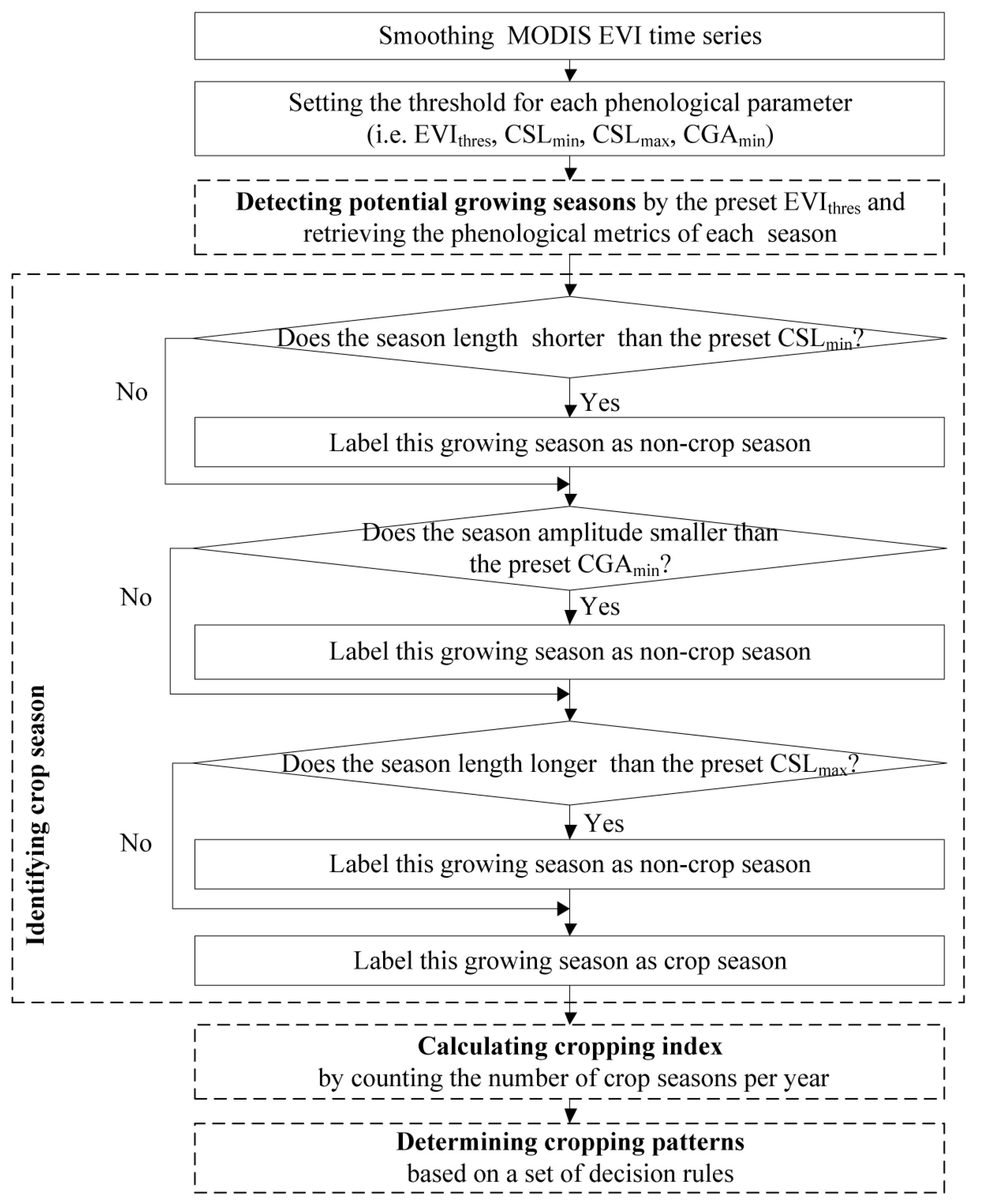
3. Methodology

The aim of this study is to map cropping patterns, focusing on major crops, such as wheat, rice, corn, soybean and cotton, while excluding fruit and tree crops (i.e., orchards and vineyards). The proposed phenology-based cropping pattern method is based on a global threshold model to retrieve phenological metrics. To execute the method, the MODIS EVI time series need to be smoothed first, followed by a proper threshold and parameter setting for extracting the phenological parameters. The four parameters/thresholds are (abbreviations in brackets):
  • EVI threshold [EVIthres]
  • The minimum crop season length [CSLmin]
  • The maximum crop season length [CSLmax]
  • The minimum crop growth amplitude [CGAmin]
The four parameters are used to determine cropping patterns using four major processing steps (Figure 3):
  • Detecting the potential growing seasons and retrieving the phenological metrics (SOS, EOS, season length and seasonal amplitude)
  • Identifying crop seasons
  • Calculating cropping index
  • Determining cropping patterns

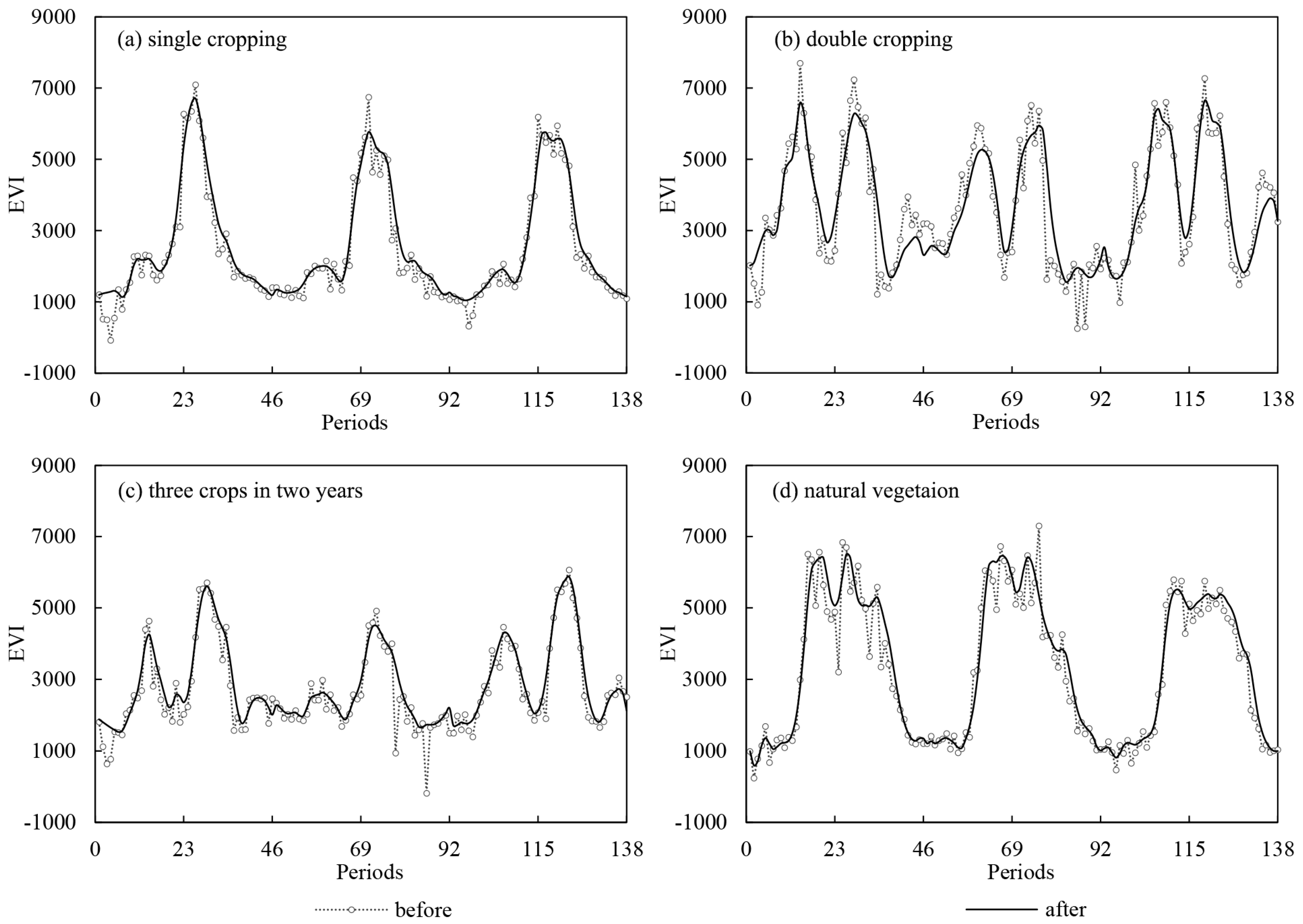
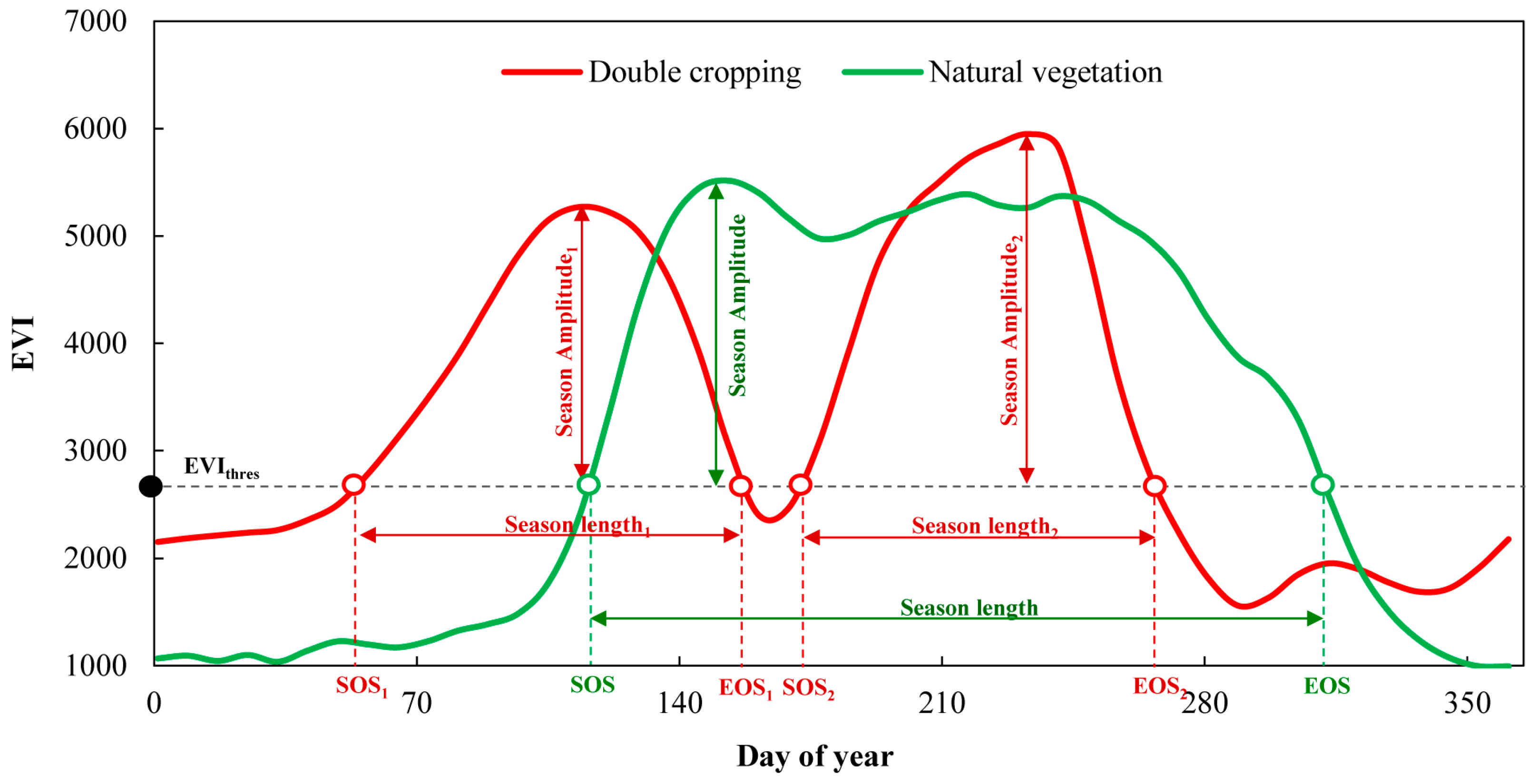
3.1. Threshold Model and Phenological Metrics

Though all vegetation in the same region present similar periodic activities (e.g., green up, maturity, senescence and dormancy), there are important growth differences between crops and natural vegetation [66]. For example, the season length of crops such as wheat, rice and corn in North China is usually shorter than that of natural vegetation (Figure 1). Phenological metrics derived from remotely sensed time-series vegetation index data have therefore been successfully used to distinguish crops from other land cover types [67,68,69].
Several models have been developed to obtain season length and season amplitude from remotely sensed time-series vegetation index data, among which the ‘threshold method’ is the most widely used [70]. In the threshold model, the start of season (SOS) is designated as the day of year (DOY) where the vegetation index crosses the preset threshold (EVIthres) in the upward phase while the end of season (EOS) is designated as the DOY where vegetation crosses the same threshold in the downward phase [71,72]. This is illustrated in Figure 4, where the typical EVI profile (red line) of double cropping and natural vegetation (green line) intersect with the predefined threshold value (broken line), which we denote as SOS and EOS, respectively. The season amplitude is defined as the difference between the maximum EVI value within a growing season (i.e., between SOS and EOS) and the threshold. Season length is defined as the time span (in days) between the SOS and EOS. Therefore, in the threshold model, once the EVIthres is set, the four phenological metrics (SOS, EOS, season length and season amplitude) of a vegetation growing season are determined. It is also obvious that the season length of natural vegetation is much longer than that of crops, which could be used to distinguish them.

3.2. Description of the PBCP Method

As outlined in Figure 3, the threshold model is used in the first step to detect growing seasons and to retrieve the phenological metrics of each season (i.e., season length and season amplitude) based on the preset EVI threshold (EVIthres). Next (step 2), the obtained season length and season amplitude are compared with the preset minimum crop season length (CSLmin), maximum crop season length (CSLmax) and minimum crop growth amplitude (CGAmin). This permits to distinguish crop seasons and non-crop seasons. In step 3, the cropping index of each pixel is calculated by counting the number of crop seasons within each year. In the final step (step 4), the cropping pattern in the current year is determined with a set of decision rules based on cropping indexes over three consecutive years.

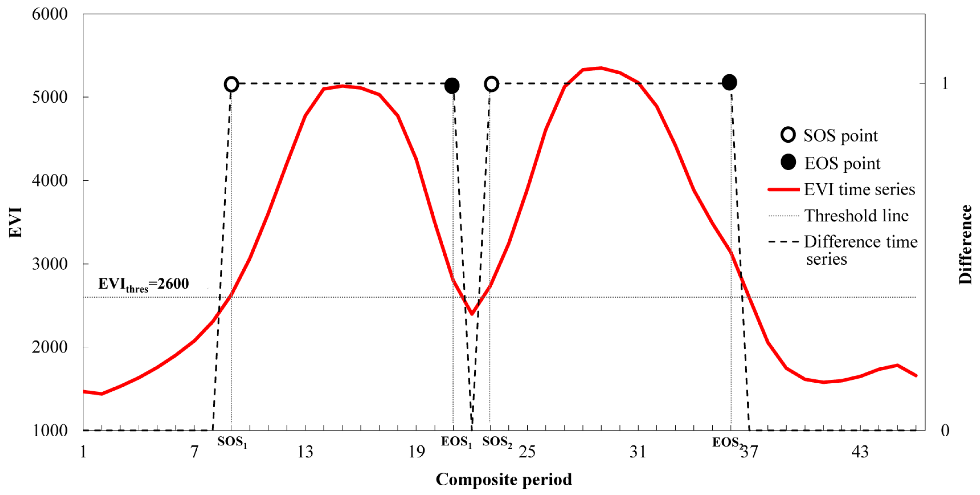
3.2.1. Detection of Potential Growing Seasons and Retrieval of Phenological Metrics

To identify whether a pixel contained any crop season, for each pixel, the number of vegetation growing seasons, the season length and season amplitude need to be derived. Figure 5 illustrates that these metrics can be readily obtained once the EVIthres is set. The illustration shows the retrieval of phenological metrics from 8-day composite EVI time series, based on the global threshold model. In our implementation, we first create a binary time series as follows:
  • 0 if EVI − EVIthres ≤ 0
  • 1 if EVI − EVIthres > 0
In the new binary time series, a growing season starts with the first encountered “1” (SOS) and ends with the last member of the consecutive string of “1” (season length). EOS is here simply the last “1” encountered within each consecutive binary string. Hence, SOS should always alternate with EOS. Possible pseudo-growth seasons are later eliminated in the crop season identification process (step 2 in Figure 3). While analyzing the binary time series, the number of vegetation growing seasons equals the number of SOS (or EOS) encountered. The season length is calculated as the time period from SOS to EOS for each season. The season amplitude, finally, is derived from the smoothed EVI time series as the difference between the maximum EVI value within a growing season and the preset EVIthres.

3.2.2. Identification of Crop Seasons

The accurate detection of cropping pattern largely depends on the recognition of crop seasons from time-series vegetation index data. Season length and season amplitude are very effective in identifying the crop season from EVI temporal profiles and to separate crop seasons from other vegetation types. Therefore, in our method, besides EVIthres, we define and subsequently optimize three conditions to identify crop seasons, that is the minimum crop season length (CSLmin), the maximum crop season length (CSLmax) and the minimum crop growth amplitude (CGAmin).
These three conditions ensure that the detected growth cycle belongs to crops. For example, to qualify as crop cycle, the length of the season should exceed a certain minimum length, as a crop needs some time to finalize its development. At the same time, the seasonal amplitude should exceed some minimum value to indicate the presence of rapid biomass accumulation, which is typical for crops. Very long cycles and/or small seasonal amplitudes, on the other hand, are untypical for crops such as wheat, rice, or corn.
Usually, the season length of cereal crops in North China is between 90 days and 120 days (Table 3). A shorter growing season either indicates seasonal vegetables or the short growing season of winter wheat before overwintering. Very short growing seasons are also typical for weeds and green covers with earlier green-up than crops. In our method, if the derived season length is shorter than the preset minimum crop season length, this season is labeled as a non-crop season. Following the same logic, the season lengths of natural vegetation, such as forest and grass/shrubland, are usually longer than that of crops. If the derived season length is longer than the preset maximum crop season length, then this growing season is labeled as a non-crop season.
The seasonal amplitude is a good indicator for crops, as crops develop from bare soil (low EVI) to full coverage (high EVI). The season amplitude is also a useful indictor to identify cropland and differentiate different crops [39]. For example, the season amplitude for winter wheat is generally between 0.3 and 0.4 EVI units, whereas the value is between 0.35 and 0.45 for maize in North China [52]. If the derived season amplitude is smaller than the preset minimum crop seasonal amplitude, then this growing season is labeled in our method as a non-crop season. The combined use of the three conditions (min/max season length and minimum seasonal amplitude) offers the possibility to identify and delete non-crop growing seasons.

3.2.3. Calculation of Cropping Index

The cropping index is defined here as the number of crops planted and harvested over a year. In this paper, the cropping index was directly calculated from the number of crop seasons within a calendar year for each pixel within the cropping extent. For any year, the maximum cropping index value was restricted to 3 because generally only up to three crops (e.g., triple cropping) can be cultivated and reaped over a year around the world.

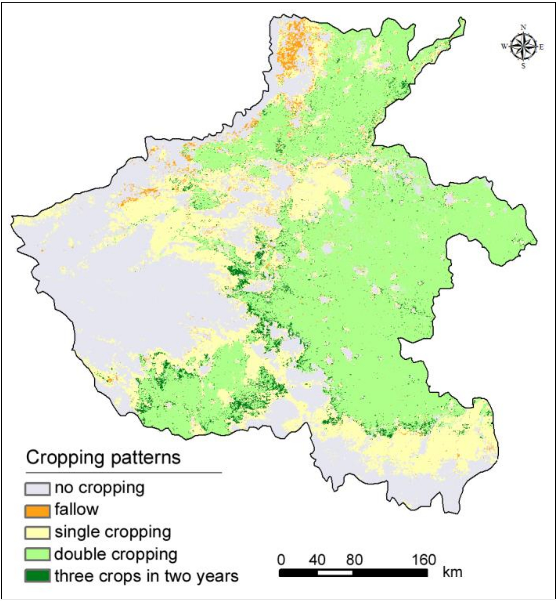
3.2.4. Determination of Cropping Patterns

In the determination of cropping patterns, it is necessary to capture the inherent variability as well as the possible land-use/land-cover changes. A cropping pattern may span more than one year, such as the pattern of three crops in two years practiced in some regions of China (Figure 1c). Furthermore, considering the possibility of non-cropland conversion to cropland and vice versa, as well as the potential of cropping intensification and fallow, it is difficult to determine cropping patterns only considering the cropping frequency in one year.
To determine the cropping patterns in the current year, we recommend to combine cropping indexes from at least three years (i.e., the previous year, the current year and the following year). The cropping pattern is determined from analysis of the three (yearly) cropping indexes. Since only up to three crops can be harvested over a year, the possible cropping index value is either 0, 1, 2, or 3. Thus, for a candidate pixel, there are 64 (i.e., 43) different combinations of cropping index for three years. We propose to distinguish five different cropping patterns:
  • No cropping
  • Fallow
  • Single cropping
  • Double cropping
  • Triple cropping
The cropping pattern for each of the 64 combinations is determined by the rules outlined in Table A1 of the Appendix A:
  • All combinations with cropping indexes of 0 in at least two consecutive years are defined as “no cropping”. Combinations with a cropping index of 0 in the current year and non-zero values in the two neighboring years are defined as “fallow”. For other combinations containing 0, their cropping patterns are determined by the cropping index of the current year (i.e., a cropping index of the current year of 1 is defined as “single cropping”, a cropping index of the current year of 2 is defined as “double cropping” and a cropping index of the current year of 3 is defined as “triple cropping”).
  • For all the remaining combinations containing 3 crop cycles, they stand for regions with agricultural potential for triple cropping. In such regions, both single cropping and double cropping are likely to be practiced. Therefore, their cropping patterns are determined by the cropping index of the current year.
  • For the remaining combinations of values of 1 and 2, two rules are used to determine their cropping patterns. The first rule is that if the cropping index for the current year is the same as either that of the former year or the following year, its cropping pattern is determined by the cropping index of the current year. The second rule is that the combinations of (2, 1, 2) and (1, 2, 1) both stand for regions reaping three crops over two years, and their cropping pattern is defined as three crops in two years.
According to the above rules, the cropping patterns for all 64 situations can be determined in an automated and transparent way.

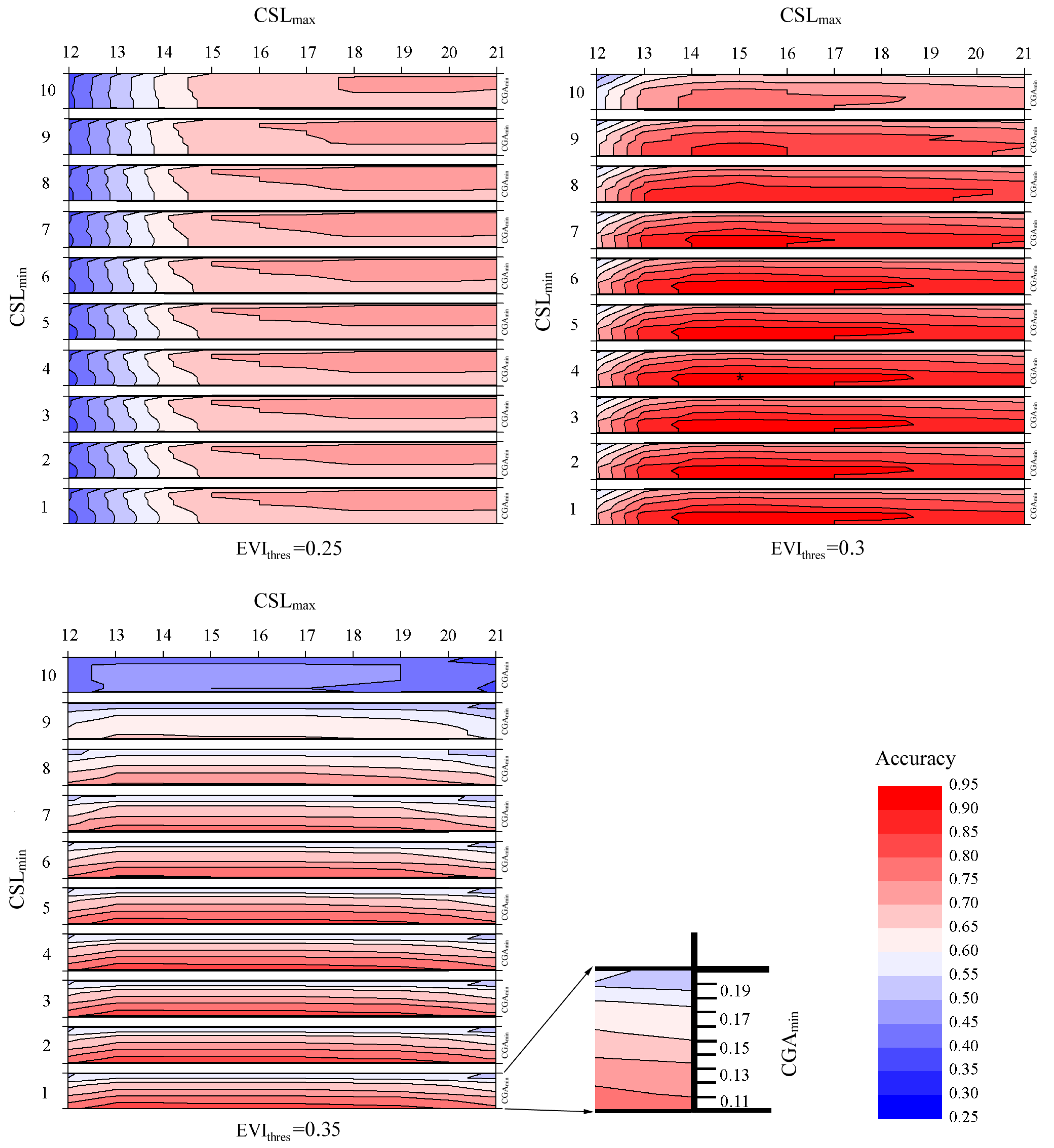
3.3. Supervised Optimization of Thresholds

Crop calendar data, such as shown in Table 3, only provide a rough guidance with respect to regional min/max crop season lengths and other thresholds involved in our method. In addition, when setting thresholds, one has also to consider that mixed pixels exist in the MODIS data. It is therefore appropriate to fix the thresholds empirically. To obtain the optimal thresholds for the four phenological parameters, we explored the sensitivity of the method to each parameter and searched for the optimal thresholds using a reference data set. If the method is to be applied in a different regional context, it is recommended to redo such a calibration.
Since the ultimate cropping pattern mapping accuracy largely depends on the extraction of the cropping index, its correct determination is the most important. To optimize the thresholds with respect to the cropping index, we randomly selected 180 training pixels from the study area (solid black dots in Figure 2). For each training sample, the number of crop seasons (i.e., cropping index) was visually interpreted by examining the shape of its EVI time series and the Landsat TM images in 2008, and then recorded and used as reference data.
In the subsequent optimization process, an exhaustive (look-up-table) search was conducted assessing all possible combinations of four parameters (ranges in parentheses together with increments):
  • EVI threshold (0.25 ≤ EVIthres ≤ 0.35 with an increment of 0.01)
  • Minimum crop season length (1 ≤ CSLmin ≤ 10 with an increment of 1, corresponding to a season length between 8 and 80 days for the 8-day composited EVI)
  • Maximum crop season length (13 ≤ CSLmax ≤ 22 with an increment of 1, corresponding to a season length between 124 and 176 days for the 8-day composited EVI)
  • Minimum crop growth amplitude (0.1 ≤ CGAmin ≤ 0.2 with an increment of 0.01).
For each test, the identified number of crop seasons for each training sample was compared with the reference data, followed by a calculation of the overall accuracy [73]. The thresholds yielding the highest overall accuracy were selected and fixed for the remaining of the study.

4. Results and Discussion

4.1. Sensitivity Analysis and Threshold Optimization

The remotely derived cropping index values show a strong sensitivity with respect to the four parameters which can be fine-tuned in our proposed method (Figure 6): EVIthres, CSLmin, CSLmax and CGAmin. Such sensitivities are expected, if one considers illustrations such as the one provided in Figure 1.
Through variations of the four parameters, strong differences in the correlation between modeled and reference cropping index are obtained. Depending on the selected thresholds, the overall accuracy of the modeled cropping index varies between 0.3 and 0.9. Figure 6 also illustrates that EVIthres has the strongest impact amongst the four parameters (only three different values for EVIthres are shown: 0.25, 0.30 and 0.35). In addition, a wide range of threshold settings can achieve satisfactory overall accuracy (above 0.85) for an average EVIthres of 0.30. Optimum parameters were identified as: EVIthres = 0.30; CSLmin = 4; CSLmax = 15 and CGAmin = 0.13. With this setting, the overall accuracy of cropping index mapping was 0.95. For all following modeling steps, this setting was kept. It is expected that the optimum calibration is region dependent.

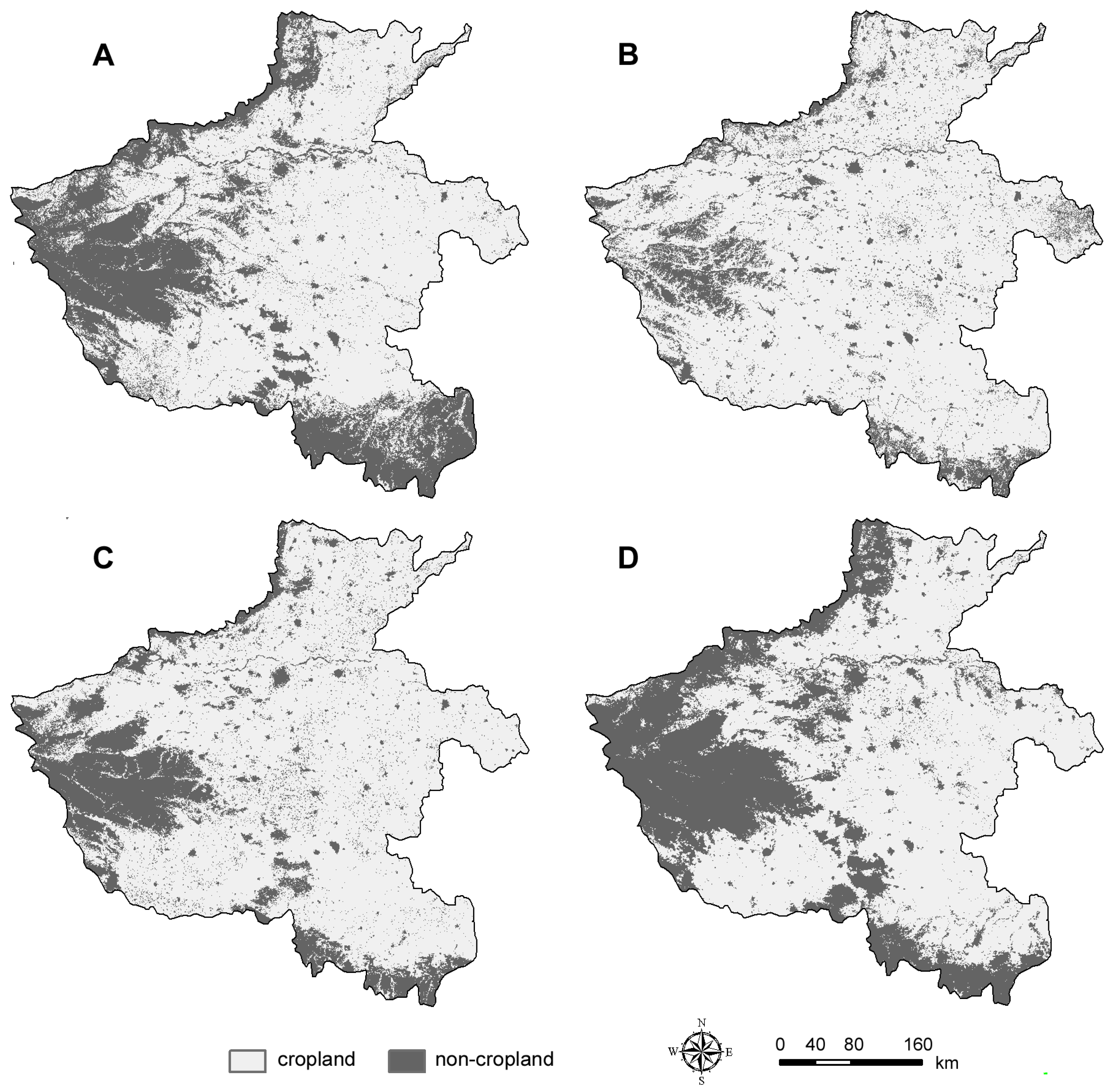
4.2. Comparisons Between the PBCP-derived Cropland Extent and Other Cropland Datasets

The PBCP method yields a cropland extent layer by merging all pixels with at least one crop season per year. To check the plausibility of the obtained map, it was compared against three reference cropland layers derived from well-known global land cover products: GCE, GC2009 and MODIS-IGBP (Figure 7). For the study area, large variations in cropland extent were observed, as already observed for example by Vancutsem et al. [74] for Africa. The largest cropland extent in Henan was 13.45 million ha from the GlobCover 2009, while our method (PBCP) predicted the smallest extent: 10.7 million ha. The cropland extents from the GCE and MODIS IGBP data were notably close to each other, that is, 12.72 million ha and 12.80 million ha, respectively.
The accuracies of the four cropland layers were quantitatively assessed using the 270 validation pixels (hollow dots in Figure 2). For each validation pixel, its cropping pattern was determined through visual interpretation of its EVI time series for 2008–2010 and the corresponding TM images (Table 4). High omission errors for cropland were found for the PBCP method (19%) and GCE (18%). The highest commission error for cropland was observed for GlobCover 2009 (17%), while the lowest was observed for PBCP (1%). Several papers have already highlighted the inconsistency of existing land cover maps [14,75,76,77]. According to those studies, the differences are mainly due to (i) different thematic class definitions, and (ii) differences in the datasets used to perform the classification.
Taking into account Table 4 as well as Figure 7, it is clear that the modeled cropland extent using the PBCP method is smaller compared to the three reference maps. We nevertheless kept the parameter setting leading to this conservative estimate of cropland extent, as we primarily aimed to map cropping patterns, and the targeted crops were mainly grain crops with a relatively long growth cycle. Seasonal vegetables with short growth cycles and nursery gardens with natural-vegetation-like growth cycles were in this context of minor importance and hence excluded. Using the proposed parameter setting, crops with such short crop cycles are classified as no crops, and this explains the observed underestimation of cropland extent (Figure 7D).

4.3. Cropping Index Extraction and Validation

Because the cropping pattern mapping accuracy is largely determined by the cropping index mapping accuracy, we compare the cropping index mapping accuracy of our MODIS-based method with that of the TM classification method. The test area is located in the center and north of Henan (Figure 8). Two Landsat TM images with Tile 124-036 on 6 April and 12 August in 2009 were used to extract cropping area in the first and second half of the year with an SVM classifier, respectively. If a pixel had crops planted both in the first and second half of the year, then its cropping index was set to 2. If a pixel had crop planted either in the first half of the year or the second half of the year, then its cropping index was set to 1. If pixel had no crop planted within the year, then its cropping index was set to 0. The cropping index mapping accuracies for the TM classification method and the PBCP method were assessed with 292 randomly selected samples (black dots in Figure 8A) of size 500 m × 500 m (similar to the size of a MODIS pixel) from the test area. Because a 500 m × 500 m sample covers 17 × 17 TM pixels, we considered the dominant cropping index of the 17 × 17 pixels as the cropping index of the validation sample.
Overall, the spatial distribution of the cropping index derived with the PBCP method (Figure 8A) agreed well with that from the TM classification result (Figure 8B). Areas with two crops in 2009 were concentrated in the south east and north of the region, and areas with one crop were mainly distributed in the central and south west of the region. The overall cropping index mapping accuracy for the PBCP method was 85.3%, whereas it was 84.5% for the TM classification method (Table 5). We nevertheless noted several discrepancies between the two cropping index data. Taking the area around pixel α (Figure 8) as an example, the cropping index from our algorithm was 1 (Figure 8A), whereas it was 0 for the TM classification result (Figure 8B). In the Landsat TM image on 6 April 2009 (Figure 8C), this area was not covered by any green vegetation. In the TM image on 12 August 2009 (Figure 8D), the vegetation reflectance signal of this area was too weak to be classified as crops. However, when observed from a high-resolution image in Google Earth (Figure 8E), the area around pixel α was cropland. Furthermore, as shown in the smoothed temporal profile (Figure 8G), apparently summer crop was planted in the area around pixel α. Therefore, we confirmed that the area around pixel α was planted with a single crop in 2009. As another example, the area around pixel β displayed the spectral characteristics of buildings in Figure 8C but displayed the spectral characteristics of dense vegetation in Figure 8D, and thus, this area was classified as single crop from the TM classification. However, this area was a nursery garden, which can also be confirmed by high-resolution Google Earth images (Figure 8F). As observed in the Google Earth maps, the texture of the nursery garden was completely different from that of crops. The smoothed temporal profile of pixel β (Figure 8H) also confirmed that it had a longer growing season from late April to early November, which was distinctly different from that of crops. Though remote sensing data of high-spatial resolution is more informative for ground details, the high temporal resolution time-series vegetation data has advantages in cropping index extraction.

4.4. Cropping Pattern Extraction and Validation

The spatial distribution of cropping patterns in Henan for 2009 is shown in Figure 9. The overall distribution derived with the PBCP method, and using the optimized parameter setting, confirms well our general knowledge of the region [78]. Five cropping patterns were distinguished in Henan, including (1) no cropping (non-cultivated area), (2) fallow, (3) single cropping, (4) double cropping and (5) the pattern of three crops in two years. Double cropping was the dominant cropping pattern in Henan. The pattern of three crops in two years scattered in the transition zones between single cropping and double cropping. Cotton, spring maize, summer maize, and rice are the prevailing crops cultivated in single cropping. Winter wheat-summer maize/peanut/soybean, rapeseed-rice are the typical crop rotations practiced in double cropping, while winter wheat-summer maize-summer maize is practiced in the pattern of three crops in two years. The accuracy assessment based on 270 reference pixels (hollow dots in Figure 2) indicated that the overall cropping pattern mapping accuracy in Henan was 84% (Table 6).
With an overall accuracy of around 84%, the proposed PBCP method compares favorably with published results [52,61,78]. However, as each region is different in terms of cropping pattern, but also field sizes and observation conditions, etc. a direct comparison of various studies is not productive. Any attempt to compare different methods should focus on identical datasets in order to separate regional and data related effects, from real methodological differences.
Our analysis also shows that the presented results still contain significant uncertainties, despite the fact that the overall accuracy of the cropping pattern mapping was satisfactory. Major problems are related to the coarse resolution of MODIS data and the complexity of cropping patterns, intertwined with sometimes relatively small field sizes [49,55,56,57].
Despite these limitations, the study highlighted the potential of the proposed phenology-based method. The method presented in this paper can be extended easily to other regions, in particular if reference data for fine-tuning of parameters are available. Similar or even better results can be expected using other datasets. For example, recently, the ability to detect temporal signals from the medium-resolution satellite HJ-1 A/B data has been explored [79]. Together with the advancement of data fusion techniques, it is now also possible to acquire higher resolution time-series data by combining decametric resolution data (such as Landsat-8 OLI) with coarse resolution time-series data (such as MODIS) [80,81,82]. Furthermore, the newly launched two twin Sentinel-2 satellites provide images with advanced spatial resolution and more rapid revisit cycle [38]. It contains 10 spectral bands from 0.4 μm to 2.4 μm with satisfactory coverage as well as three bands for atmospheric correction and cloud detection. The most desirable feature about Sentinel-2 data is that its spatial resolution is up to 10 m and the revisit period is only 10 days. If combined, the two satellites provide continuous observation of earth surface at an interval of five days. This is a huge advantage compared to other satellite data, which makes it the most favorable data source in regional agricultural land use mapping, especially for regions with fractional landscapes. Nevertheless, for retrospective analyses, a continued research in the use of hecto/kilo-metric time series as offered by MODIS or AVHRR is highly warranted [2,11,36].
Therefore, it is promising to map crop types, cropping intensity, cropping patterns and cropping practice in great special detail with phonological signals from high-resolution time-series data in the near future.

5. Conclusions

This paper proposed a phenology-based method to map cropland extent and cropping pattern based on time-series Enhanced Vegetation Index (EVI) data. The proposed method utilizes four phenological parameters to detect vegetation seasons, retrieve phenological metrics, and identify crop seasons. Based on those crop seasons, cropping patters are identified using a set of decision rules considering cropping indexes in three consecutive years. The method was applied in China’s Henan province to map its cropping patterns in 2009. Results show that: (1) the cropping extent generated from the PBCP method was of moderate accuracy (78%) but slightly conservative. (2) The cropping index mapping accuracy with the PBCP method was comparable with that from Landsat-5 TM image classification. (3) The overall cropping pattern mapping accuracy of Henan province in 2009 was satisfactory with an overall accuracy of 84% (kappa: 0.79), assessed using 270 independent validation samples. Together, these findings demonstrate that information about cropland extent, number of crop seasons (e.g., cropping index) and cropping pattern can be obtained in a cost-efficient way, over large areas, using coarse resolution (MODIS) time series. As vegetation index time series from coarse resolution sensors extend back to the 1980s, our method offers the prospect of being applicable in retrospective analyses, yielding important information about agricultural land use characteristics, otherwise difficult to obtain from higher resolution sensors such as Landsat.
Two aspects of the PBCP method need to be addressed and investigated in the future. The first is that we used a global threshold to retrieve phenological metrics. The selected threshold will affect the retrieved cropping pattern, as the cropping index value is directly dependent on it. To improve the mapping accuracy, a local threshold is likely to be adopted in the further development of the PBCP method. The second recommended improvement relates to the decision rules brought forward for the determination of cropping patterns. In setting up these rules, many situations were considered, especially the possible changes of land-use status and the patterns, which extend over multiple years. With this set of decision rules, the cropping patterns were determined immediately from the cropping index data. As some situations may not have been considered in our rule set, we recommend to further refine and improve the decision rules.

Author Contributions

J.L. and W.Z. developed the method; X.H. collected and processed the data; J.L. implemented the method; A.Z. validated the results and contributed to data analysis; Y.P. supervised the work; C.A. contributed with significant advice, and editing of the paper.

Funding

This research was founded by National Natural Science Foundation of China (NO. 41401494), China Postdoctoral Science Foundation (NO. 2014M552475), Foundation of Shaanxi Educational Committee (NO. 14JK1745), and Program of Education Department of Hebei Province (NO. BJ2018043).

Conflicts of Interest

The authors declare no conflict of interest.

Appendix A

Table A1. Look-up table for cropping patterns in accordance with different cropping index combinations.
NO.Cropping Index in Year − 1Cropping Index in the Current YearCropping Index in Year + 1Cropping Pattern of the Current YearNO.Cropping Index in Year − 1Cropping Index in the Current YearCropping Index in Year + 1Cropping Pattern of the Current Year
1000no cropping33200no cropping
2001no cropping34201fallow
3002no cropping35202fallow
4003no cropping36203fallow
5010single cropping37210single cropping
6011single cropping38211single cropping
7012single cropping39212three crops in two years
8013single cropping40213single cropping
9020double cropping41220double cropping
10021double cropping42221double cropping
11022double cropping43222double cropping
12023double cropping44223double cropping
13030triple cropping45230triple cropping
14031triple cropping46231triple cropping
15032triple cropping47232triple cropping
16033triple cropping48233triple cropping
17100no cropping49300no cropping
18101fallow50301fallow
19102fallow51302fallow
20103fallow52303fallow
21110single cropping53310single cropping
22111single cropping54311single cropping
23112single cropping55312single cropping
24113single cropping56313single cropping
25120double cropping57320double cropping
26121three crops in two years58321double cropping
27122double cropping59322double cropping
28123double cropping60323double cropping
29130triple cropping61330triple cropping
30131triple cropping62331triple cropping
31132triple cropping63332triple cropping
32133triple cropping64333triple cropping

References

  1. FAO. Agro-ecological Zoning: Guidelines. In FAO Soils Bulletiin 7; Food and Agriculture Organisation of the United Nations: Rome, Italy, 1996. [Google Scholar]
  2. Bégué, A.; Arvor, D.; Bellon, B.; Betbeder, J.; de Abelleyra, D.; Ferraz, R.P.D.; Lebourgeois, V.; Lelong, C.; Simões, M.; Verón, S.R. Remote sensing and cropping practices: A review. Remote Sens. 2018, 10, 99. [Google Scholar] [CrossRef]
  3. Foley, J.A.; DeFries, R.; Asner, G.P.; Barford, C.; Bonan, G.; Carpenter, S.R.; Chapin, F.S.; Coe, M.T.; Daily, G.C.; Gibbs, H.K.; et al. Global consequences of land use. Science 2005, 309, 570–574. [Google Scholar] [CrossRef] [PubMed]
  4. Cassman, K.G.; Wood, S. Cultivated systems. In Ecosystems and Human Well-Being: Current State and Trends; Hassan, R., Ed.; Island Press: Washington, DC, USA, 2005; Volume 1, pp. 747–794. [Google Scholar]
  5. Fan, M.X.; MacKenzie, A.F.; Cadrin, F. Nitrous oxide emission in three years as affected by tillage, corn-soybean-alfalfa rotations, and nitrogen fertilization. J. Environ. Qual. 1998, 27, 698–703. [Google Scholar]
  6. Millar, N.; Robertson, G.P.; Grace, P.R.; Gehl, R.J.; Hoben, J.P. Nitrogen fertilizer management for nitrous oxide (N2O) mitigation in intensive corn (Maize) production: An emissions reduction protocol for US Midwest agriculture. Mitig. Adapt. Strategy Glob. Chang. 2010, 15, 185–204. [Google Scholar] [CrossRef]
  7. Snyder, C.S.; Bruulsema, T.W.; Jensen, T.L.; Fexin, P.E. A Review of greenhouse gas emissions from crop production systems and fertilizer management effects. Agric. Ecosyst. Environ. 2009, 133, 247–266. [Google Scholar] [CrossRef]
  8. Wanyama, I.; Rufino, M.C.; Pelster, D.E.; Wanyama, G.; Atzberger, C.; Asten, P.; Verchot, L.V.; Butterbach-Bahl, K. Land use, land use history, and soil type affect soil greenhouse gas fluxes from agricultural landscapes of the East African Highlands. J. Geophys. Res. Biogeosci. 2018, 123, 976–990. [Google Scholar] [CrossRef]
  9. Thenkabail, P.S. Global croplands and their importance for water and food security in the twenty-first century: Towards an ever green revolution that combines a second green revolution with a blue revolution. Remote Sens. 2010, 2, 2305–2312. [Google Scholar] [CrossRef]
  10. Foley, J.A.; Ramankutty, N.; Brauman, K.A.; Cassidy, E.S.; Gerber, J.S.; Johnston, M.; Mueller, N.D.; O’Connell, C.; Ray, D.K.; West, P.C.; et al. Solutions for a cultivated planet. Nature 2011, 478, 337–372. [Google Scholar] [CrossRef] [PubMed]
  11. Atzberger, C. Advances in remote sensing of agriculture: Context description, existing operational monitoring systems and major information needs. Remote Sens. 2013, 5, 949–981. [Google Scholar] [CrossRef]
  12. Bellón, B.; Bégué, A.; Lo Seen, D.; de Almeida, A.C.; Simões, M. A remote sensing approach for regional-scale mapping of agricultural land-use systems based on NDVI time series. Remote Sens. 2017, 9, 600. [Google Scholar] [CrossRef]
  13. Gray, J.; Friedl, M.; Frolking, S.; Ramankutty, N.; Nelson, A.; Gumma, M.K. Mapping Asian cropping intensity with MODIS. IEEE J. Sel. Top. Appl. Earth Obs. Remote Sens. 2014, 7, 3373–3379. [Google Scholar] [CrossRef]
  14. Waldner, F.; Fritz, S.; Di Gregorio, A.; Defourny, P. Mapping priorities to focus cropland mapping activities: Fitness assessment of existing global, regional and national cropland maps. Remote Sens. 2015, 7, 7959–7986. [Google Scholar] [CrossRef] [Green Version]
  15. Friedl, M.A.; McIver, D.K.; Hodges, J.C.F.; Zhang, X.Y.; Muchoney, D.; Strahler, A.H.; Woodcock, C.E.; Gopal, S.; Schneider, A.; Cooper, A.; et al. Global land cover mapping from MODIS: Algorithms and early results. Remote Sens. Environ. 2002, 83, 287–302. [Google Scholar] [CrossRef]
  16. Friedl, M.A.; Sulla-Menashe, D.; Tan, B.; Schneider, A.; Ramankutty, N.; Sibley, A.; Huang, X. MODIS collection 5 global land cover: Algorithm refinements and characterization of new datasets. Remote Sens. Environ. 2010, 114, 168–182. [Google Scholar] [CrossRef]
  17. Chen, J.; Chen, J.; Liao, A.; Cao, X.; Chen, L.; Chen, X.; He, C.; Han, G.; Peng, S.; Lu, M. Global land cover mapping at 30 m resolution: A POK-based operational approach. ISPRS J. Photogramm. Remote Sens. 2015, 103, 7–27. [Google Scholar] [CrossRef]
  18. Chen, J.; Cao, X.; Peng, S.; Ren, H. Analysis and applications of globeland30: A review. ISPRS Int. J. Geoinf. 2017, 6, 230. [Google Scholar] [CrossRef]
  19. Bontemps, S.; Defourny, P.; Van Bogaert, E.; Arino, O.; Kalogirou, V.; Perez, J.R. GLOBCOVER2009: Products Description and Validation Report; European Spatial Agency and Université Catholique de Louvain: Frascati, Italy, 2011; Available online: http://due.esrin.esa.int/files/GLOBCOVER2009_Validation_Report_2.2.pdf (accessed on 3 July 2018).
  20. Li, W.; MacBean, N.; Ciais, P.; Defourny, P.; Lamarche, C.; Bontemps, S.; Houghton, R.A.; Peng, S. Gross and net land cover changes in the main plant functional types derived from the annual ESA CCI land cover maps (1992–2015). Earth Syst. Sci. Data 2018, 10, 219–234. [Google Scholar] [CrossRef] [Green Version]
  21. Bartholome, E.; Belward, A. GLC2000: A new approach to global land cover mapping from earth observation data. Int. J. Remote Sens. 2005, 26, 1959–1977. [Google Scholar] [CrossRef]
  22. Loveland, T.; Reed, B.; Brown, J.; Ohlen, D.; Zhu, Z.; Yang, L.; Merchant, J. Development of a global land cover characteristics database and IGBP DISCover from 1 km AVHRR data. Int. J. Remote Sens. 2000, 21, 1303–1330. [Google Scholar] [CrossRef] [Green Version]
  23. Thenkabail, P.S.; Biradar, C.M.; Noojipady, P.; Dheeravath, V.; Li, Y.J.; Velpuri, M.; Gumma, M.; Reddy, G.P.O.; Turral, H.; Cai, X.L.; et al. Global irrigated area map (GIAM), derived from remote sensing, for the end of the last millennium. Int. J. Remote Sens. 2009, 30, 3679–3733. [Google Scholar] [CrossRef]
  24. Biradar, C.M.; Thenkabail, P.S.; Noojipady, P.; Li, Y.J.; Dheeravath, V.; Turral, H.; Velpuri, M.; Gumma, M.K.; Gangalakunta, O.R.P.; Cai, X.L.; et al. A global map of rainfed cropland areas (GMRCA) at the end of last millennium using remote sensing. Int. J. Appl. Earth Obs. Geoinf. 2009, 11, 114–129. [Google Scholar] [CrossRef]
  25. Pittman, K.; Hansen, M.C.; Becker-Reshef, I.; Potapov, P.V.; Justice, C.O. Estimating global cropland extent with multi-year MODIS data. Remote Sens. 2010, 2, 1844–1863. [Google Scholar] [CrossRef]
  26. Xiong, J.; Thenkabail, P.S.; Tilton, J.C.; Gumma, M.K.; Teluguntla, P.; Congalton, R.G.; Yadav, K.; Dungan, J.; Oliphant, A.J.; Poehnelt, J.; et al. NASA Making Earth System Data Records for Use in Research Environments (MEaSUREs) Global Food Security-Support Analysis Data (GFSAD) @ 30-m Africa: Cropland Extent Product (GFSAD30AFCE); NASA EOSDIS Land Processes DAAC, USGS Earth Resources Observation and Science (EROS) Center: Sioux Falls, SD, USA, 2017. [CrossRef]
  27. Xiong, J.; Thenkabail, P.S.; Tilton, J.C.; Gumma, M.K.; Teluguntla, P.; Oliphant, A.; Congalton, R.G.; Yadav, K.; Gorelick, N. Nominal 30-m cropland extent map of continental Africa by integrating pixel-based and object-based algorithms using sentinel-2 and Landsat-8 Data on Google Earth Engine. Remote Sens. 2017, 9, 1065. [Google Scholar] [CrossRef]
  28. Teluguntla, P.; Thenkabail, P.S.; Xiong, J.; Gumma, M.K.; Congalton, R.G.; Oliphant, A.J.; Sankey, T.; Poehnelt, J.; Yadav, K.; Massey, R.; et al. NASA Making Earth System Data Records for Use in Research Environments (MEaSUREs) Global Food Security-Support Analysis Data (GFSAD) @ 30-m for Australia, New Zealand, China, and Mongolia: Cropland Extent Product (GFSAD30AUNZCNMOCE); NASA EOSDIS Land Processes DAAC, USGS Earth Resources Observation and Science (EROS) Center: Sioux Falls, SD, USA, 2017. [CrossRef]
  29. Oliphant, A.J.; Thenkabail, P.S.; Teluguntla, P.; Xiong, J.; Congalton, R.G.; Yadav, K.; Massey, R.; Gumma, M.K.; Smith, C. NASA Making Earth System Data Records for Use in Research Environments (MEaSUREs) Global Food Security-Support Analysis Data (GFSAD) @ 30-m for Southeast & Northeast Asia: Cropland Extent Product (GFSAD30SEACE); NASA EOSDIS Land Processes DAAC, USGS Earth Resources Observation and Science (EROS) Center: Sioux Falls, SD, USA, 2017. [CrossRef]
  30. Gumma, M.K.; Thenkabail, P.S.; Teluguntla, P.; Oliphant, A.J.; Xiong, J.; Congalton, R.G.; Yadav, K.; Phalke, A.; Smith, C. NASA Making Earth System Data Records for Use in Research Environments (MEaSUREs) Global Food Security-Support Analysis Data (GFSAD) @ 30-m for South Asia, Afghanistan and Iran: Cropland Extent Product (GFSAD30SAAFGIRCE); NASA EOSDIS Land Processes DAAC, USGS Earth Resources Observation and Science (EROS) Center: Sioux Falls, SD, USA, 2017. [CrossRef]
  31. Phalke, A.; Ozdogan, M.; Thenkabail, P.S.; Congalton, R.G.; Yadav, K.; Massey, R.; Teluguntla, P.; Poehnelt, J.; Smith, C. NASA Making Earth System Data Records for Use in Research Environments (MEaSUREs) Global Food Security-Support Analysis Data (GFSAD) @ 30-m for Europe, Middle-East, Russia and Central Asia: Cropland Extent Product (GFSAD30EUCEARUMECE); NASA EOSDIS Land Processes DAAC, USGS Earth Resources Observation and Science (EROS) Center: Sioux Falls, SD, USA, 2017. [CrossRef]
  32. Massey, R.; Sankey, T.T.; Yadav, K.; Congalton, R.G.; Tilton, J.C.; Thenkabail, P.S. NASA Making Earth System Data Records for Use in Research Environments (MEaSUREs) Global Food Security-Support Analysis Data (GFSAD) @ 30 m for North America: Cropland Extent Product (GFSAD30NACE); NASA EOSDIS Land Processes DAAC, USGS Earth Resources Observation and Science (EROS) Center: Sioux Falls, SD, USA, 2017. [CrossRef]
  33. Zhong, Y.; Giri, C.; Thenkabail, P.S.; Teluguntla, P.; Congalton, R.G.; Yadav, K.; Oliphant, A.J.; Xiong, J.; Poehnelt, J.; Smith, C. NASA Making Earth System Data Records for Use in Research Environments (MEaSUREs) Global Food Security-Support Analysis Data (GFSAD) @ 30-m for South America: Cropland Extent Product (GFSAD30SACE); NASA EOSDIS Land Processes DAAC, USGS Earth Resources Observation and Science (EROS) Center: Sioux Falls, SD, USA, 2017. [CrossRef]
  34. Congalton, R.G.; Yadav, K.; McDonnell, K.; Poehnelt, J.; Stevens, B.; Gumma, M.K.; Teluguntla, P.; Thenkabail, P.S. NASA Making Earth System Data Records for Use in Research Environments (MEaSUREs) Global Food Security-Support Analysis Data (GFSAD) @ 30-m: Cropland Extent Validation (GFSAD30VAL); NASA EOSDIS Land Processes DAAC, USGS Earth Resources Observation and Science (EROS) Center: Sioux Falls, SD, USA, 2017. [CrossRef]
  35. Teluguntla, P.; Thenkabail, P.; Xiong, J.; Gumma, M.K.; Giri, C.; Milesi, C.; Ozdogan, M.; Congalton, R.; Yadav, K. Global food security support analysis data at nominal 1 km (GFSAD1km) derived from remote sensing in support of food security in the twenty-first century: Current achievements and future possibilities. In Land Resources Monitoring, Modeling, and Mapping with Remote Sensing; Thenkabail, P.S., Ed.; CRC Press: Boca Raton, FL, USA; London, UK; New York, NY, USA, 2015; Chapter 6; Volume 2, pp. 131–160. ISBN 978-148-221-795-7. [Google Scholar]
  36. Becker-Reshef, I.; Justice, C.; Sullivan, M.; Vermote, E.; Tucker, C.; Anyamba, A.; Small, J.; Pak, E.; Masuoka, E.; Schmaltz, J.; et al. Monitoring Global croplands with coarse resolution earth observations: The global agriculture monitoring (GLAM) project. Remote Sens. 2010, 2, 1589–1609. [Google Scholar] [CrossRef]
  37. Congalton, G.R.; Gu, J.; Yadav, K.; Thenkabail, P.; Ozdogan, M. Global land cover mapping: A review and uncertainty analysis. Remote Sens. 2014, 6, 12070–12093. [Google Scholar] [CrossRef]
  38. Inglada, J.; Arias, M.; Tardy, B.; Hagolle, O.; Valero, S.; Morin, D.; Dedieu, G.; Sepulcre, G.; Bontemps, S.; Defourny, P.; et al. Assessment of an operational system for crop type map production using high temporal and spatial resolution satellite optical imagery. Remote Sens. 2015, 7, 12356–12379. [Google Scholar] [CrossRef]
  39. Matton, N.; Canto, S.G.; Waldner, F.; Valero, S.; Morin, D.; Inglada, J.; Arias, M.; Bontemps, S.; Koetz, B.; Defourny, P. An automated method for annual cropland mapping along the season for various globally-distributed agrosystems using high spatial and temporal resolution time series. Remote Sens. 2015, 7, 13208–13232. [Google Scholar] [CrossRef]
  40. Atzberger, C.; Vuolo, F.; Klisch, A.; Rembold, F.; Meroni, M.; Mello, M.P.; Formaggio, A. Agriculture. In Remote Sensing Handbook (Volume 2): Land Resources Monitoring, Modeling, and Mapping with Remote Sensing; Thenkabail, P.S., Ed.; CRC Press: Boca Raton, FL, USA, 2016; Volume 2, pp. 71–112. [Google Scholar]
  41. Thenkabail, P.S.; Wu, Z. An automated cropland classification algorithm (ACCA) for Tajikistan by combining Landsat, MODIS, and secondary data. Remote Sens. 2012, 4, 2890–2918. [Google Scholar] [CrossRef]
  42. Lambert, M.; Waldner, F.; Defourny, P. Cropland mapping over Sahelian and Sudanian Agrosystems: A knowledge-based approach using PROBA-V time series at 100-m. Remote Sens. 2016, 8, 232. [Google Scholar] [CrossRef]
  43. Waldner, F.; Lambert, M.; Li, W.; Weiss, M.; Demarez, V.; Morin, D.; Marais-Sicre, C.; Hagolle, O.; Baret, F.; Defourny, P. Land cover and crop type classification along the season based on biophysical variables retrieved from multi-sensor high-resolution time series. Remote Sens. 2015, 7, 10400–10424. [Google Scholar] [CrossRef]
  44. Inglada, J.; Vincent, A.; Arias, M.; Marais-Sicre, C. Improved early crop type identification by joint use of high temporal resolution SAR and optical image time series. Remote Sens. 2016, 8, 362. [Google Scholar] [CrossRef]
  45. Baghdadi, N.; Cresson, R.; Todoroff, P.; Moinet, S. Multitemporal observations of sugarcane by TerraSAR-X images. Sensors 2010, 10, 8899–8919. [Google Scholar] [CrossRef] [PubMed] [Green Version]
  46. Marais Sicre, C.; Inglada, J.; Fieuzal, R.; Baup, F.; Valero, S.; Cros, J.; Huc, M.; Demarez, V. Early detection of summer crops using high spatial resolution optical image time series. Remote Sens. 2016, 8, 591. [Google Scholar] [CrossRef]
  47. Inglada, J.; Vincent, A.; Arias, M.; Tardy, B.; Morin, D.; Rodes, I. Operational high resolution land cover map production at the country scale using satellite image time series. Remote Sens. 2017, 9, 95. [Google Scholar] [CrossRef]
  48. Immitzer, M.; Vuolo, F.; Atzberger, C. First experience with Sentinel-2 data for crop and tree species classifications in central Europe. Remote Sens. 2016, 8, 166. [Google Scholar] [CrossRef]
  49. Singh, N.J.; Kudrat, M.; Jain, K.; Pandey, K. Cropping pattern of Uttar Pradesh using IRS-P6 (AWiFS) data. Int. J. Remote Sens. 2011, 32, 4511–4526. [Google Scholar] [CrossRef]
  50. Valero, S.; Morin, D.; Inglada, J.; Sepulcre, G.; Arias, M.; Hagolle, O.; Dedieu, G.; Bontemps, S.; Defourny, P.; Koetz, B. Production of a dynamic cropland mask by processing remote sensing image series at high temporal and spatial resolutions. Remote Sens. 2016, 8, 55. [Google Scholar] [CrossRef]
  51. Wardlow, B.D.; Kastens, J.H.; Egbert, S.L. Using USDA crop progress data for the evaluation of greenup onset date calculated from MODIS 250-meter data. Photogramm. Eng. Remote Sens. 2006, 11, 1225–1234. [Google Scholar] [CrossRef]
  52. Liu, J.; Zhu, W.; Cui, X. A shape-matching cropping index (CI) mapping method to determine agricultural cropland intensities in China using MODIS time-series data. Photogramm. Eng. Remote Sens. 2012, 78, 829–837. [Google Scholar] [CrossRef]
  53. Atzberger, C.; Eilers, P.H.C. A time series for monitoring vegetation activity and phenology at 10-daily time steps covering large parts of South America. Int. J. Digit. Earth 2011, 4, 365–386. [Google Scholar] [CrossRef]
  54. Sakamoto, T.; Nguyen, N.V.; Ohno, H.; Ishitsuka, N.; Yokozawa, M. Spatio-temporal distribution of rice phenology and cropping systems in the Mekong Delta with special reference to the seasonal water flow of the Mekong and Bassac rivers. Remote Sens. Environ. 2006, 100, 1–6. [Google Scholar] [CrossRef]
  55. Galford, G.L.; Mustard, J.F.; Melillo, J.; Gendrin, A.; Cerri, C.C.; Cerri, C.E.P. Wavelet analysis of MODIS time series to detect expansion and intensification of row-crop agriculture in Brazil. Remote Sens. Environ. 2008, 112, 576–587. [Google Scholar] [CrossRef]
  56. Lv, T.; Liu, C. Study on extraction of crop information using time-series MODIS data in the Chao Phraya Basin of Thailand. Adv. Space Res. 2010, 45, 775–784. [Google Scholar]
  57. Sakamoto, T.; Van Phung, C.; Kotera, A.; Nguyen, K.D.; Yokozawa, M. Analysis of rapid expansion of inland aquaculture and triple rice-cropping areas in a coastal area of the Vietnamese Mekong Delta using MODIS time-series imagery. Landsc. Urban Plan. 2009, 92, 34–46. [Google Scholar] [CrossRef]
  58. Jönsson, P.; Eklundh, L. TIMESAT—A program for analyzing time-series of satellite sensor data. Comput. Geosci. 2004, 30, 833–845. [Google Scholar] [CrossRef]
  59. Eklundh, L.; Jönsson, P. TIMESAT for processing time-series data from satellite sensors for land surface monitoring. In Multitemporal Remote Sensing: Methods and Applications; Ban, Y., Ed.; Springer International Publishing: Cham, Switzerland, 2016; pp. 177–194. [Google Scholar]
  60. Han, M. Planting system and geographical difference of corn in China during the past 300 years. Geogr. Res. 2006, 25, 1083–1095, (In Chinese with English abstract). [Google Scholar]
  61. Mulianga, B.; Bégué, A.; Clouvel, P.; Todoroff, P. Mapping Cropping practices of a sugarcane-based cropping system in Kenya using remote sensing. Remote Sens. 2015, 7, 14428–14444. [Google Scholar] [CrossRef] [Green Version]
  62. National Bureau of Statistics of China. China Statistical Yearbook 2011; China Statistics Press: Beijing, China, 2016.
  63. Huete, A.; Didan, K.; Miura, T.; Rodriguez, E.P.; Gao, X.; Ferreira, L.G. Overview of the radiometric and biophysical performance of the MODIS vegetation indices. Remote Sens. Environ. 2002, 83, 195–213. [Google Scholar] [CrossRef]
  64. Zhu, W.; Pan, Y.; He, H.; Wang, L.; Mou, M.; Liu, J. A changing-weight filter method for reconstructing a high-quality NDVI time series to preserve the integrity of vegetation phenology. IEEE Trans. Geosci. Remote Sens. 2012, 50, 1085–1094. [Google Scholar] [CrossRef]
  65. Atkinson, P.M.; Jeganathan, C.; Dash, J.; Atzberger, C. Inter-comparison of four models for smoothing satellite sensor time-series data to estimate vegetation phenology. Remote Sens. Environ. 2012, 123, 400–417. [Google Scholar] [CrossRef]
  66. Roehrig, J.; Thamm, H.; Menz, G.; Porembski, S.; Orthmann, B. A phenological classification approach for the Upper Oueme in Benin using Spot Vegetation. In Proceedings of the Second International VEGETATION User Conference, Antwerp, Belgium, 24–26 March 2004; pp. 301–306. [Google Scholar]
  67. Pan, Y.; Li, L.; Zhang, J.; Liang, S.; Zhu, X.; Sulla-Menashe, D. Winter wheat area estimation from MODIS-EVI time series data using the Crop Proportion Phenology Index. Remote Sens. Environ. 2012, 119, 232–242. [Google Scholar] [CrossRef]
  68. Zhong, L.; Gong, P.; Biging, G.S. Phenology-based crop classification algorithm and its implications on agricultural water use assessments in California’s Central Valley. Photogramm. Eng. Remote Sens. 2012, 78, 799–813. [Google Scholar] [CrossRef]
  69. Wardlow, B.D.; Egbert, S.L. Large-area crop mapping using time-series MODIS 250m NDVI data: An assessment for the U.S. Central Great Plains. Remote Sens. Environ. 2008, 112, 1096–1116. [Google Scholar] [CrossRef]
  70. De Beurs, K.M.; Henebry, G.M. Spatio-temporal statistical methods for modelling land surface phenology. In Phenological Research: Methods for Environmental and Climate Change Analysis; Hudson, I.L., Keatley, M.R., Eds.; Springer: Dordrecht, The Netherlands, 2010; pp. 177–208. [Google Scholar]
  71. White, M.A.; Beurs, K.M.; Didan, K.; Inouye, D.W.; Richardson, A.D.; Jensen, O.P.; O’Keefe, J.; Zhang, G.; Nemani, R.R.; van Leeuwen, W.; et al. Intercomparison, interpretation, and assessment of spring phenology in North America estimated from remote sensing for 1982–2006. Glob. Chang. Biol. 2009, 15, 2335–2359. [Google Scholar] [CrossRef]
  72. Zhou, L.; Tucher, C.J.; Kaufmann, R.K.; Slayback, D.; Shabanov, N.V.; Myneni, R.В. Variations in northern vegetation activity inferred from satellite data of vegetation index during 1981 to 1999. J. Geophys. Res. 2001, 106, 20069–20083. [Google Scholar] [CrossRef] [Green Version]
  73. Story, M.; Congalton, R. Accuracy assessment: A user’s perspective. Photogramm. Eng. Remote Sens. 1986, 52, 397–399. [Google Scholar]
  74. Vancutsem, C.; Marinho, E.; Kayitakire, F.; See, L.; Fritz, S. Harmonizing and combining existing land cover/land use datasets for cropland area monitoring at the African continental scale. Remote Sens. 2013, 5, 19–41. [Google Scholar] [CrossRef] [Green Version]
  75. Wu, W.; Shibasaki, R.; Yang, P.; Ongaro, L.; Zhou, Q.; Tang, H. Validation and comparison of 1 km global land cover products in China. Int. J. Remote Sens. 2008, 29, 3769–3785. [Google Scholar] [CrossRef]
  76. Pérez-Hoyos, A.; Rembold, F.; Kerdiles, H.; Gallego, J. Comparison of global land cover datasets for cropland monitoring. Remote Sens. 2017, 9, 1118. [Google Scholar] [CrossRef]
  77. Fritz, S.; See, L. Identifying and quantifying uncertainty and spatial disagreement in the comparison of Global Land Cover for different applications. Glob. Chang. Biol. 2008, 14, 1057–1075. [Google Scholar] [CrossRef]
  78. Li, L.; Friedl, M.A.; Xin, Q.; Gray, J.; Pan, Y.; Frolking, S. Mapping crop cycles in China using MODIS-EVI time series. Remote Sens. 2014, 6, 2473–2493. [Google Scholar] [CrossRef]
  79. Pan, Z.; Huang, J.; Zhou, Q.; Wang, L.; Cheng, Y.; Zhang, H.; Blackburn, G.A.; Yan, J.; Liu, J. Mapping crop phenology using NDVI time-series derived from HJ-1 A/B data. Int. J. Appl. Earth Obs. Geoinf. 2015, 34, 188–197. [Google Scholar] [CrossRef] [Green Version]
  80. Li, L.; Zhao, Y.; Fu, Y.; Pan, Y.; Yu, L.; Xin, Q. High resolution mapping of cropping cycles by fusion of Landsat and MODIS data. Remote Sens. 2017, 9, 1232. [Google Scholar] [CrossRef]
  81. Xin, Q.; Olofsson, P.; Zhu, Z.; Tan, B.; Woodcock, C.E. Toward near real-time monitoring of forest disturbance by fusion of MODIS and Landsat data. Remote Sens. Environ. 2013, 135, 234–247. [Google Scholar] [CrossRef]
  82. Chen, X.; Liu, M.; Zhu, X.; Chen, J.; Zhong, Y.; Cao, X. “Blend-then-Index” or “Index-then-Blend”: A theoretical analysis for generating high-resolution NDVI time series by STARFM. Photogramm. Eng. Remote Sens. 2018, 84, 65–73. [Google Scholar] [CrossRef]
Figure 1. Exemplary growth cycles of (a) single cropping, (b) double cropping and (c) three crops in two years. Also shown is (d) the growth cycle of natural vegetation. Examples are from North China and are based on the 8-d MODIS EVI time series during three years (46 periods per year). The dots and broken lines display the original EVI observations, while the black lines show the EVI time series after smoothing.
Remotesensing 10 01203 g001
Figure 2. Location and topography of the study area Henan province. Also indicated are the locations of training (n = 180) and validation samples (n = 270).
Remotesensing 10 01203 g002
Figure 3. Flowchart of the phenology-based cropping pattern (PBCP) mapping method. EVIthres: EVI threshold; CSLmin: the minimum crop season length; CSLmax: the maximum crop season length; CGAmin: the minimum crop growth amplitude.
Remotesensing 10 01203 g003
Figure 4. A schematic diagram illustrating the retrieval of phenological metrics using the threshold model. EVIthres: EVI threshold; SOS: start of growing season; EOS: end of growing season.
Remotesensing 10 01203 g004
Figure 5. Illustration of retrieving phenological metrics from a 8-day composite EVI time series based on the threshold model. Left-hand side y-axis: smoothed EVI time series; right-hand side y-axis: binary time series with observations < EVIthres coded as zero, and otherwise coded as one.
Remotesensing 10 01203 g005
Figure 6. Cropping index mapping accuracies under different threshold sets. The overall accuracy (Story & Congalton, 1986) is calculated between the reference cropping index and the modeled cropping index. EVIthres: EVI threshold; CSLmin: the minimum crop season length; CSLmax: the maximum crop season length; CGAmin: the minimum crop growth amplitude. Optimum parameters (marked by *) were identified as: EVIthres = 0.30; CSLmin = 4; CSLmax = 15 and CGAmin = 0.13. Note that only results for three EVIthres values are shown here, while the complete range between 0.25 and 0.35 (with increments of 0.01) were investigated.
Remotesensing 10 01203 g006
Figure 7. Croplands in Henan province derived from three different data sources and our method. (A) The 250-m Global Cropland Extent product. (B) The 300-m GlobCover map. (C) The 500-m MODIS-IGBP. (D) The 500-m cropping extent generated by the proposed PBCP method (this paper).
Remotesensing 10 01203 g007
Figure 8. Comparisons between the cropping indexes derived from the PBCP method and the TM classification. (A) The cropping index derived from the MODIS EVI time series with the PBCP method. Black dots denote the validation samples. (B) The classification results derived from multi-temporal Landsat TM images. (C) Landsat TM image (RGB: 7-4-3) on 6 April 2009. (D) Landsat TM image (RGB: 7-4-3) on 12 August 2009. (E) The Google Earth image showing the area around pixel α on 27 December 2009. (F) The Google Earth image showing the texture differences between nursery garden (area around pixel β) and crops on 11 May 2008. (G) The temporal profile of the EVI data for pixel α. (H) The temporal profile of the EVI data for pixel β.
Remotesensing 10 01203 g008
Figure 9. Spatial distribution of cropping patterns in Henan derived with the PBCP method in 2009.
Remotesensing 10 01203 g009
Table 1. List of the widely-used land cover products produced from earth observation data with global coverage.
ProductAgriculture Related InformationExtentPeriodUpdating FrequencyMain Data SourceResolutionReferences
MCD12Q1Cropland extentGlobal2001–2016AnnuallyEOS-MODIS500 m[15,16]
GlobeLand30Cropland extentGlobalCirca2000, Circa2010No updateLandsat TM/ETM+, HJ-130 m[17,18]
GlobCover 2009Cropland extentGlobal2009No updateENVISAT MERIS300 m[19]
CCI Land CoverCropland extentGlobal1992–2015AnnuallyNOAA-AVHRR, SPOT-VGT, ENVISAT-MERIS, ENVISAT-ASAR, PROBA-V300 m[20]
GLC2000Cropland extentGlobal2000No updateSPOT-VGT1000 m[21]
IGBP-DISCoverCropland extentGlobal1992–1993No updateNOAA-AVHRR1000 m[22]
GIAMExtent of irrigated croplandGlobalcirca 2000No updateNOAA-AVHRR1000 m[23]
GMRCAExtent of rainfed croplandGlobalcirca 2000No updateNOAA-AVHRR, SPOT-VGT1000 m[24]
GLECropland extentGlobalcirca 2000No updateEOS-MODIS250 m[25]
GFSAD30Cropland extentGlobalNominal year 2015No updateLandsat OLI/ETM+, Sentinel MSI, SRTM30 m[26,27,28,29,30,31,32,33,34,35]
Table 2. Information on the Landsat-5 images (cloud cover < 10%) used in this study.
Path/RowDateCloud Cover Percentage (%)
124/0362 March 20080
12 October 20085
6 April 20091
12 August 20090
11 May 20100
28 June 20107
124/0372 March 20080
12 October 20082
6 April 20092
25 June 20090
11 May 20100
Table 3. Phenological stages of major crops in Henan Province, China, in 2010.
MonthJanFebMarAprilMayJunJulAugSepOctNovDec
Ten-DayEMLEMLEMLEMLEMLEMLEMLEMLEMLEMLEMLEML
Winter wheat 1444443566/788/99/1010/1111/1212 11/22/334
Summer maize 2 1/22/33/444/566/77/889
Soybean 3 1/22/333/44/55/66/7789
Peanut 4 1/22/33/44567
Cotton 5 11/2233/4455/666/77/88/9
1 Winter wheat: 1—Sowing, 2—Seeding, 3—Tillering, 4—Overwintering, 5—Green up, 6—Jointing, 7—Booting, 8—Heading, 9—Stem elongation, 10—Milk ripening, 11—Maturing,12—Harvesting; 2 Summer Maize: 1—Sowing, 2—Three leaves, 3—Seven leaves, 4—Jointing, 5—Tasseling, 6—Stem elongation, 7—Milk ripening, 11—Maturing, 12—Harvesting; 3 Soybean: 1—Sowing, 2—Seeding, 3—Three leaves, 4—Branches forming, 5—Flowering, 6—Pod setting, 7—Seed filling, 8—Maturing, 12—Harvesting; 4 Peanut: 1—Sowing, 2—Seeding, 3—Three leaves, 4—Flowering, 5—Pod swelling, 6—Maturing, 7—Harvesting; 5 Cotton: 1—Sowing, 2—Seeding, 3—Three leaves, 4—Five leaves, 5—Squaring, 6—Flowering, 7—Boll opening, 8—Harvesting, 9—Stop growing.
Table 4. Accuracy assessment for the four cropland maps in Henan Province.
Cropland ProductCategoryProducer’s AccuracyOmission ErrorUser’s AccuracyCommission ErrorOverall Accuracy
GCENon-cropland78%22%58%42%81%
Cropland82%18%92%8%
GlobCover 2009Non-cropland40%60%65%35%80%
Cropland93%7%83%17%
MODIS-IGBPNon-cropland51%49%72%28%83%
Cropland94%6%86%14%
PBCP method (this paper)Non-cropland98%2%52%48%78%
Cropland71%19%99%1%
Table 5. Confusion matrix for the cropping indexes derived with the PBCP method (MODIS data) and the classification result from TM images based on 292 random samples of size 500 m × 500 m in the test area.
Reference DataOverall AccuracyKappa
CI = 0CI = 1CI = 2Total
TMCI = 0121161013784.6%0.75
CI = 10321951
CI = 2009494
Total12148123292
MODISCI = 075908485.3%0.77
CI = 117501784
CI = 200124124
Total9259141292
CI = 0 for no crop, CI = 1 for one crop, CI = 2 for two crops.
Table 6. Confusion matrix for the cropping patterns in Henan province derived with the PBCP method in 2009.
Reference Data
No CroppingFallowSingle CroppingDouble CroppingThree Crops/Two YearsTotalUser’s Accuracy
PBCPno cropping79013409682%
fallow21110402740%
single cropping2052305791%
double cropping00072072100%
three crops/two years0003151883%
Total8311758615270
Producer’s Accuracy95%100%69%83%100%
Overall accuracy = 84%, Kappa = 0.79

